The DEEP2 Galaxy Redshift Survey: The evolution of the blue fraction in groups and the field

Abstract

We explore the behavior of the blue galaxy fraction over the redshift range $0.75\leq z\leq 1.3$ in the DEEP2 Survey, both for field galaxies and for galaxies in groups. The primary aim is to determine the role that groups play in driving the evolution of galaxy colour at high $z$. In pursuing this aim, it is essential to define a galaxy sample that does not suffer from redshift-dependent selection effects in colour-magnitude space. We develop four such samples for this study: at all redshifts considered, each one is complete in colour-magnitude space, and the selection also accounts for evolution in the galaxy luminosity function. These samples will also be useful for future evolutionary studies in DEEP2. The colour segregation observed between local group and field samples is already in place at $z\sim 1$: DEEP2 groups have a significantly lower blue fraction than the field. At fixed $z$, there is also a correlation between blue fraction and galaxy magnitude, such that brighter galaxies are more likely to be red, both in groups and in the field. In addition, there is a negative correlation between blue fraction and group richness. In terms of evolution, the blue fraction in groups and the field remains roughly constant from $z=0.75$ to $z\sim 1$, but beyond this redshift the blue fraction in groups rises rapidly with $z$, and the group and field blue fractions become indistinguishable at $z\sim 1.3$. Careful tests indicate that this effect does not arise from known systematic or selection effects. To further ensure the robustness of this result, we build on previous mock DEEP2 catalogues to develop mock catalogues that reproduce the colour-overdensity relation observed in DEEP2 and use these to test our methods. The convergence between the group and field blue fractions at $z\sim 1.3$ implies that DEEP2 galaxy groups only became efficient at quenching star formation at $z\sim 2$; this result is broadly consistent with other recent observations and with current models of galaxy evolution and hierarchical structure growth.

1 Introduction

One of the most striking characteristics of the galaxy population is the well-known environmental segregation of the two main galaxy types: red, early-type galaxies with little ongoing star formation preferentially occur in galaxy groups and clusters, while blue, late-type galaxies with significant star-formation activity avoid such systems and preferentially populate the “field”. This observation has been recognized as a key to understanding galaxy formation and evolution for more than fifty years (Spitzer & Baade, 1951).

There is now overwhelming evidence that the galaxy population in clusters has evolved significantly with redshift down to the present day. Butcher & Oemler (1984) were the first to present evidence that the fraction of blue galaxies, $f_{b}$, in clusters increases strongly with increasing $z$—the so-called Butcher-Oemler (BO) effect. This basic result—an increased incidence of star-forming galaxies in distant clusters—has been replicated in numerous later studies using a variety of star-formation indicators, including cluster blue fractions (Rakos & Schombert, 1995; Margoniner & de Carvalho, 2000; Kodama & Bower, 2001; Ellingson et al., 2001; Margoniner et al., 2001), emission-line galaxy fractions (Poggianti et al., 2006), and morphological fractions (Oemler et al., 1997; Couch et al., 1998; van Dokkum et al., 2000; Fasano et al., 2000; Lubin et al., 2002; Goto et al., 2003). Such studies have also been extended to less massive galaxy groups (Allington-Smith et al., 1993; Wilman et al., 2005; Martínez et al., 2006), which also appear to have proportionally more star-forming galaxies back in time. To be sure, there remain strong reasons to question the veracity of the BO effect as it was originally presented for galaxies in the cores of rich clusters (e.g., Koo 1988; Smail et al. 1998; Andreon et al. 2006). But it is now indisputable that clusters, on the whole, had proportionally more blue, star-forming, and morphologically late-type galaxies—in short, more star formation—at $z\sim 0.5$ than they do at present.

It is tempting to conclude that this evolution is responsible for the substantial growth that has been observed in the number density of red galaxies since $z\sim 1$ (Bell et al., 2004b; Willmer et al., 2006; Faber et al., 2006). But it is also important to note that, in addition to evolution within the group and cluster environment, the build-up of the red galaxy population could also be driven by an increasing number density of groups and clusters from the growth of structure. We shall try in this paper to shed light on the relative importance in DEEP2 of these two channels for red-galaxy formation.

A blue fraction that declines with time in groups and clusters is a natural consequence of hierarchical schemes for galaxy formation (Kauffmann, 1995; Baugh et al., 1996; Diaferio et al., 2001; Benson et al., 2001) if one assumes that groups and clusters play a role in quenching star formation. Since these systems form at relatively late times, their member galaxies at intermediate redshift will have had less time, on average, to “feel” the effects of group membership; thus, a smaller fraction of them will have ceased forming stars. Indeed, it has been shown (Kodama & Bower, 2001) that the evolution of $f_{b}$ in clusters out to $z\sim 0.4$ can be entirely accounted for by considering the effects of hierarchical structure formation and a declining universal star-formation rate. For exactness in what follows, then, we shall use the phrase “Butcher-Oemler effect” to refer just to this effect—a decline in the typical blue fraction in groups and clusters that results simply from the increasing age of these systems with time, and not from any evolution in the quenching efficiency of groups and clusters. Although this working definition differs somewhat from the effect originally reported by Butcher & Oemler (1984), it reflects usage that has become common in recent literature. It is also worth noting that, under this definition, the BO effect may be stronger in some types of systems than in others (in clusters than in groups, for example), depending on the accretion rates and quenching efficiencies involved.

It remains unclear, however, which specific physical mechanisms are responsible for quenching star formation, over what timescales they act, and even whether these mechanisms are peculiar to groups and clusters. A variety of mechanisms has been proposed, including (1) galaxy mergers (e.g, Toomre & Toomre 1972), which occur primarily in galaxy groups (e.g., Cavaliere et al. 1992) and can trigger AGN feedback that sweeps merger remnants of their gas (Springel et al. 2005); (2) close, high-velocity galaxy encounters (“harrassment”; Moore et al. 1996), which occur primarily in clusters; (3) ram-pressure stripping of galaxy gas by the hot intracluster medium (Gunn & Gott 1972); and (4) the less violent process known as “strangulation” in which gas accretion onto galaxy discs is cut off, either by stripping of galaxies’ gaseous haloes (Larson et al. 1980) or by feedback from low-luminosity AGN (Croton et al., 2006), and star formation ends when the remaining supply of gas has been exhausted. There is evidence that each of these processes is at work on some level; it may be that no single mechanism bears primary responsibility for galaxy evolution. Disentangling how and to what degree each of the above processes shapes the galaxy population requires detailed observations of galaxies over a wide range of redshifts and environments.

The observed evolution is rather complicated in its details, however. For example, the well-known morphology-density relation for galaxies in clusters (e.g., Dressler 1980) and groups (e.g. Postman & Geller 1984) evolves strongly with increasing redshift (Dressler et al., 1997), and there is evidence that the evolution in intermediate-density environments has occured more recently than in high-density environments (Smith et al., 2005). It also appears that the morphological mix of cluster early-types has changed with time (Fasano et al., 2000; Postman et al., 2005). Complicating things further, cluster blue fractions display a substantial system-to-system scatter at all epochs (Butcher & Oemler, 1984; Smail et al., 1998; Margoniner & de Carvalho, 2000; Goto et al., 2003; De Propris et al., 2004). This scatter can be ascribed in part to the observed trends between blue fraction and cluster mass, i.e., velocity dispersion (Newberry et al., 1988), inferred virial mass (Martínez et al., 2002), richness (Margoniner et al., 2001; Goto et al., 2003; Tovmassian et al., 2005), or total optical luminosity (Weinmann et al., 2006a); the correlation between $f_{b}$ and mass also appears to evolve with redshift (Poggianti et al., 2006). The scatter may also arise in part from a correlation between $f_{b}$ and a cluster’s degree of dynamical relaxation (e.g., Metevier et al. 2000). The scatter in $f_{b}$ might mask or enhance the redshift evolution, depending on the cluster selection criteria used (Newberry et al., 1988; Andreon & Ettiori, 1999). Indeed, Smail et al. (1998) observe no BO effect out to $z\sim 0.25$ in a sample of luminous X-ray clusters (but see also Fairley et al. 2002), and many authors have commented on the presence of individual massive clusters at high redshift with low $f_{b}$ and well-formed red sequences (e.g. Koo 1981; Homeier et al. 2005; Andreon 2006). It is clear that a robust study of galaxy evolution in groups and clusters requires a sample that contains a broad range of systems and is uniformly selected at all redshifts.

Until relatively recently, studies of galaxy evolution in clusters were limited to cluster samples pre-selected from optical imaging or X-ray maps; such samples are prone to selection effects that bias the galaxy sample as a function of $z$. The advent of large, densely sampled galaxy redshift surveys like the 2-degree Field Galaxy Redshift Survey (2dFGRS) and the Sloan Digital Sky Survey (SDSS), however, has allowed selection of large, low-redshift cluster samples directly from the galaxy distribution in redshift space, where redshift-dependent selection effects can be well understood and accounted for. Several authors have studied the properties of the cluster galaxy population in the 2dFGRS (Balogh et al., 2004; De Propris et al., 2004) and SDSS (Goto, 2005a, b; Weinmann et al., 2006a; Quintero et al., 2006). Within SDSS, there have even been detections of an evolving $f_{b}$ in clusters (Goto et al., 2003; Martínez et al., 2006) and of an evolving morphology-density relation (Goto et al., 2004). With the high-redshift DEEP2 Galaxy Redshift Survey (Davis et al. 2004, Faber et al. in prep.) nearing completion, it is now possible to extend these studies to $z\sim 1$.

DEEP2 has now yielded a catalogue of several thousand groups and small clusters over a wide range of masses at $z\sim 1$ (Gerke et al., 2005). A study of the DEEP2 sample by Cooper et al. (2006b) has already revealed that, without explicitly considering groups, the correlations between galaxy properties and the density of the nearby galaxy distribution are qualitatively similar at $z\sim 1$ to what is observed locally (e.g., Balogh et al. 2004; Hogg et al. 2004), although the relations differ in detail. Interestingly, recent studies have shown that these correlations evolve with redshift, becoming stronger over time (Nuijten et al., 2005; Cucciati et al., 2006; Cooper et al., 2006a), and that the color-density relation in the local Universe can be ascribed almost entirely to mechanisms acting in groups and clusters (Blanton et al., 2006). The primary goal of this paper, then, is to establish the role that groups and clusters play, if any, in driving the evolution of the DEEP2 galaxy population. In particular, we shall explore the possibility that group and cluster environments are responsible for the build-up of red galaxies observed over the DEEP2 redshift range (Bell et al., 2004b; Willmer et al., 2006; Faber et al., 2006); by so doing, we will try to shed light on the physical mechanisms driving the evolution. Although this study will focus on the evolutionary effects of galaxies’ membership in groups and clusters (that is to say, of their dark matter halo masses), there is important complementary information to be gained by studying the effects of the local density of galaxies. Such a study is undertaken in a companion paper to this one by Cooper et al. (2006a). For now, however, we will measure $f_{b}$ for galaxies in groups and clusters, as a function of redshift, and compare it to that found in the general field (i.e., in the galaxy population outside of groups). We will also investigate the relation between $f_{b}$ and cluster properties in order to gain insight into the processes at work and also to understand and control any systematic selection effects.

The thoughtful reader may find it perverse to use the blue fraction to study the evolution of red galaxies, but $f_{b}$ has significant historical precedent in the study of cluster galaxy populations, so we use it for consistency with earlier studies. In any case, the possibly more natural red fraction statistic is simply $f_{r}=1-f_{b}$. We have chosen to consider galaxy colour rather than other indicators of galaxy type like morphology or [O II] line emission primarily because it can be measured accurately for the largest number of DEEP2 galaxies, allowing for robust statistics. The DEEP2 ground-based imaging lacks the resolution necessary for morphological classification of most galaxies at $z\sim 1$, and there is HST imaging for only a small fraction of the sample. Emission line strength can be measured accurately only in spectra with sufficient signal-to-noise ratio; not all DEEP2 galaxies meet this criterion. Also, it has recently been shown that [O II] emission may not give a clear indication of star formation, especially in red galaxies (Yan et al., 2006). Regardless, there is a strong and relatively tight correlation between [O II] equivalent width and galaxy colour(e.g., Weiner 2005; Cooper et al. 2006b), so the two statistics should give similar results.

We shall proceed as follows. In §2, we describe the DEEP2 survey and the DEEP2 group catalogue, and in §3 we discuss the construction of mock DEEP2 galaxy catalogues appropriate for this study. We describe our galaxy selection criteria and incompleteness corrections and present the precise definition of $f_{b}$ used here in §4. Measurements of $f_{b}$ in groups and the field are presented in §5, and we perform tests with the mock catalogues in § 6. We discuss the implications of our results for galaxy evolution models in §7, and in §8 we summarize our results and conclusions. Readers uninterested in the details of our selection methods and robustness checks should skip to §§ 4.1, 5 and 7. Throughout the paper we assume a flat, $\Lambda$CDM cosmology with $\Omega_{M}=0.3$.

2 The DEEP2 Galaxy Redshift Survey

2.1 Details of the Survey

The DEEP2 Galaxy Redshift Survey is the first large, highly accurate spectroscopic survey of galaxies at redshifts around unity. As of this writing, the main survey observations are nearly complete ($>95\%$), with spectra obtained for $49,220$ galaxies in four fields using the DEIMOS spectrograph on the Keck II telescope. The survey covers a total of $\sim 3\;\mathrm{deg}^{2}$ on the sky to limiting magnitude $R_{AB}=24.1$. The bulk of these observations are of galaxies in the redshift range $0.7\la z\la 1.4$. Full details of the survey will appear in the upcoming paper by Faber et al. (in preparation), but summarize the necessary information for this study is summarized below.

The four fields surveyed were chosen to lie in zones of low Galactic extinction using the dust maps of Schlegel et al. (1998). Three-band ($BRI$) photometry was obtained for each field using the CFH12K camera on the Canada-France-Hawaii Telescope, as described by Coil et al. (2004a). Each field is covered by several contiguous photometric pointings, which are a convenient way to group and intercompare results. Three of the DEEP2 fields each cover an area $90^{\prime}$ or $130^{\prime}\times 30^{\prime}$ on the sky with two or three contiguous pointings. In these fields, galaxies are selected for spectroscopy using a simple cut in $BRI$ colour-colour space that has been optimized to select galaxies at redshifts $z>0.75$. This cut efficiently focuses the survey on high-redshift galaxies: it reduces the portion of the spectroscopic sample at redshifts $z<0.75$ to roughly $10\%$ while discarding only $\sim 3\%$ of objects at $z>0.75$ (Faber et al. in preparation). Within each CFHT pointing, galaxies are selected for spectroscopic observation if it is possible to place them on one of the $\sim 40$ DEIMOS slit masks covering that pointing. Slit masks are tiled in an overlapping chevron pattern using an adaptive algorithm to increase the coverage in dense regions on the sky, giving nearly every galaxy two chances to be placed on a mask. Further details of the observing scheme are given in Davis et al. (2004); overall DEEP2 targets $\sim 60\%$ of galaxies that meet its selection criteria.

The fourth field of the survey, the Extended Groth Strip (hereafter EGS), covers $120^{\prime}\times 16^{\prime}$ on the sky. A concerted effort is underway by a large consortium of observing teams (the AEGIS team; Davis et al. 2006) to obtain a wide array of observations of this field from X-ray to radio wavelengths. Therefore, to maximize the evolutionary information that will be available, galaxies in the EGS have been targeted for spectroscopy regardless of estimated redshift, and at a significantly higher sampling rate than in other fields: each galaxy in EGS has four chances to be selected for observation rather than two. This means that galaxies selected for spectroscopy in the EGS constitute a superset of galaxies that would have been selected using the criteria of the other three DEEP2 fields; hence it is possible to create a high-redshift subsample of the EGS whose selection (including sampling rate) is identical to that of the rest of the DEEP2 survey. We will include this subsample in the present study.

At this writing, spectroscopic observations have been completed for all three of the high-redshift DEEP2 fields and for more than three-quarters of the EGS field. All DEEP2 spectra have been reduced using an automated data-reduction pipeline (Cooper et al. in preparation), and redshift identifications are all confirmed visually. Rest-frame $U-B$ colours and absolute $B$ magnitudes are computed using the K-correction algorithm described in Appendix A of Willmer et al. (2006). This study uses data from all of the DEEP2 CFHT pointings for which spectroscopic observations have been completed. In each pointing, the fraction of the spectra that yield a successful redshift is greater than $70\%$.

2.2 The Group Catalogue

The details of the DEEP2 group-finding procedure are fully discussed in Gerke et al. (2005); we have now applied this procedure to the full current DEEP2 dataset, which is significantly larger than that used in the previous paper. We summarize the salient points of the group-finding algorithm here.

Groups of galaxies in the DEEP2 sample are identified using the Voronoi-Delaunay Method (VDM) group finder, which was originally implemented by Marinoni et al. (2002). This group finder searches adaptively for groups (bound, virialized associations of two or more observed galaxies) using information about local density derived from the Voronoi partition and Delaunay complex of a given three-dimensional galaxy sample. Gerke et al. (2005) calibrated the VDM group finder using the mock catalogues of Yan et al. (2003), achieving the primary goal of accurately reconstructing the bivariate distribution $n(\sigma,z)$ of groups as a function of redshift and velocity dispersion for dispersions $\sigma\geq 350\mathrm{\;km\;s^{-1}}$.

For the purposes of this paper, however, we will be considering the properties of galaxies, rather than group properties, so we will focus on somewhat different measures of success here. In particular, this paper studies properties of the population of galaxies within groups (the group sample) and of the population of isolated galaxies (the field sample), so it is crucial to determine the success of the VDM at identifying each of these populations. By testing the VDM group finder on mock DEEP2 catalogues, Gerke et al. (2005) showed that the fraction of real group members that are successfully identified as such (the galaxy success rate, $S_{\mathrm{gal}}$) is $0.79$. Conversely, the fraction of galaxies in the reconstructed group population that are actually misclassified field galaxies (the interloper fraction, $f_{I}$) is $0.46$. In addition, $82\%$ of field galaxies are correctly identified, while only $6\%$ of the reconstructed field sample is made up of misclassified group members. Both samples (group and field) are thus dominated by correctly classified galaxies, but each sample is contaminated by galaxies from the other. Therefore, any differences between the group and field galaxies should be somewhat stronger in reality than what the VDM reconstructs. As will be discussed below in § 4.1, the contamination of the group sample is particularly bad for groups with velocity dispersion below $100\mathrm{\;km\;s^{-1}}$, so we will reclassify galaxies in these groups as field galaxies.

Finally, it is important to note here that groups in the DEEP2 survey are typically of modest mass. The mock catalogues of Yan et al. (2003) indicate that the bulk of the DEEP2 groups should have virial masses in the range $5\times 10^{12}\la M_{\mathrm{vir}}\la 5\times 10^{13}M_{\odot}$ ($200\la\sigma_{v}\la 400\mathrm{\;km\;s^{-1}}$), with very few groups having $M_{\mathrm{vir}}>10^{14}M_{\odot}$; this is consistent with the estimates of the minimum group mass derived from the autocorrelation function of DEEP2 groups (Coil et al., 2006). In what follows, then, any conclusions drawn about the properties of groups should not be taken to apply to rich clusters.

3 Mock Catalogues

The study of groups and clusters of galaxies is fraught with unavoidable sources of systematic error. For example, it has been shown (Szapudi & Szalay, 1996) that an error-free cluster catalogue is not achievable for an incompletely sampled galaxy distribution, even if the physical distances to the galaxies are known. Moreover, in a redshift survey the peculiar velocities of galaxies induce distortions in the redshift-space distribution of galaxies, mixing the positions of galaxies in groups with the positions of isolated galaxies and making accurate group detection even more difficult. Because of these unavoidable sources of systematic error, robust conclusions require that we test our methods on realistic mock galaxy catalogues.

Gerke et al. (2005) tested and calibrated their group-finding methods with the mock catalogues of Yan et al. (2003). These catalogues were produced by populating dark-matter-only N-body simulations with galaxies following a halo model prescription that follows Yang et al. (2003). In particular, the mocks are populated using a conditional luminosity function, $\phi(L|M)$, that assigns galaxies to a halo of mass $M$ according to a luminosity function whose parameters depend on $M$. The parameters of the model were chosen to be consistent with the two-point correlation function $\xi(r)$ observed in early DEEP2 data (Coil et al., 2004b) and with the local $\xi(r)$ from Peacock et al. (Peacock et al., 2001). These mocks were sufficient for the purpose of testing our overall success at reconstructing groups, but they do not provide information about galaxy properties aside from luminosity.

In the current work we shall need to test our success at reproducing the colours of the group galaxy population; this requires mock catalogues that include that information. The mocks must also reproduce any dependences of the galaxy colour distribution on local overdensity, since that is the trend we aim to probe in the data. To this end, we assign colours to mock galaxies by drawing colours from galaxies in similar environments within the actual DEEP2 data. This method is similar to, but less sophisticated than, the one used by Wechsler et al. (in preparation) to create the mock SDSS catalogues that were used to test the C4 group-finding algorithm (Miller et al., 2005).

The procedure is as follows. Local galaxy density in the DEEP2 data is measured by computing the distance (projected on the sky) to each galaxy’s third-nearest neighbor within $1000\mathrm{\;km\;s^{-1}}$ in redshift, as detailed in Cooper et al. (2005). DEEP2 galaxies contaminated by edge effects are discarded, and the data sample is limited to galaxies in the range $0.8<z<1.0$ to minimize the effect of the apparent magnitude limit. In the mock catalogue, local density is estimated using the projected distance to the seventh-nearest neighbor (within a catalogue of an enhanced spatial extent, to avoid edge effects in the final catalogue). The seventh-nearest neighbor in the complete, volume-limited mock catalogue has been shown to be a reasonable analogue to the third-nearest neighbor measured in the more sparsely sampled magnitude-limited data (Cooper et al., 2005). We then divide both the mock and data samples into quintiles of local density and identify each quintile in the data with the quintile in the mock that has the same local-density rank. The colour distributions within each density bin in the data can then be used to assign colours to the mock galaxies. For example, the $20\%$ of mock galaxies with the highest local densities will be assigned colours randomly drawn from the observed colour distribution of the highest-density $20\%$ of DEEP2 galaxies.

Before doing this, however, we also divide the samples by luminosity, since DEEP2 galaxy colour is observed to be correlated with luminosity (see, e.g., Willmer et al. 2006). For the DEEP2 data, we sort galaxies into four bins in absolute $B$ band magnitude. To ensure that similar parts of the luminosity function are being considered at all $z$, we shift these bins with redshift to account for evolution in the typical galaxy magnitude $M^{\ast}$. (Faber et al., 2006) found that this value evolves as $M^{\ast}\propto Qz$, with $Q=-1.37$; we apply the same linear function of $z$ to our luminosity binning of the data. The bins include only galaxies brighter than $M_{B}-5\log{h}+Q(z-1)=-20$, since the sample is incomplete for fainter magnitudes (see Figure 2), and each bin is 0.5 magnitudes wide, except for the brightest bin, which includes all galaxies brighter than $M_{B}-5\log{h}+Q(z-1)=-21.5$. The mock catalogue is divided into the same four bins, except that in this case the bins evolve with redshift as $M\propto Q_{\mathrm{mock}}z$, with $Q_{\mathrm{mock}}=-1$, the $M^{\ast}$ evolution parameter that was assumed in Yan et al. (2003). Also the faintest bin in the mocks includes all galaxies fainter than $M_{B}+Q_{\mathrm{mock}}(z-1)=-20.5$, which means that all mock galaxies fainter than this limit will have the same colour distribution as DEEP2 galaxies in the range $-20.5<M_{B}-Q(z-1)<-20$. This is the best that can be done using this procedure, since the DEEP2 sample is incomplete for fainter objects; in any event, most of the mock galaxies in this regime will fall below the DEEP2 apparent magnitude limit, so there is little practical effect.

Having divided the samples thus into bins of local overdensity and absolute magnitude, we then add colours to the mock population by considering galaxies in each bin separately. For each mock galaxy in a given luminosity-density bin, a real galaxy is selected at random from the corresponding bin in the DEEP2 data sample, and we assign that galaxy’s rest-frame $U-B$ colour to the mock galaxy in question. This procedure produces a distribution in $M_{B}$ vs. $U-B$ colour-magnitude space that matches the distribution observed in DEEP2 reasonably well (see Figure 1). Because the procedure only uses DEEP2 galaxies in the range $0.8<z<1.0$ and because it does not divide the samples by redshift, any intrinsic evolution in the colours of DEEP2 galaxies will not be reproduced in the mock catalogues. This is desirable, however, since it will allow us to confirm that our selection and group-finding procedures have not introduced any spurious evolutionary trends.

Using the colours assigned to the mock galaxies, it is possible to the K-correction procedure described in Willmer et al. (2006) to assign each galaxy an $R$-band apparent magnitude, which can be used to select mock galaxies with the same $R<24.1$ apparent magnitude limit that is used in DEEP2. In addition to this magnitude limit, we also apply the DEEP2 DEIMOS slitmask-making algorithm to the mock catalogue, as projected on the sky, removing those galaxies that would not be targeted for observation. Finally, we dilute the remaining galaxy sample to reproduce the $\sim 70\%$ redshift success rate of the survey; the dilution procedure accounts for the slight magnitude dependence of this rate.

Figure 1: Colour-magnitude and colour-redshift diagrams for the DEEP2 survey and for the mock catalogues described in the text. To aid comparison, the mock sample has been randomly diluted to contain the same number of galaxies as the data set, and each of the two data plots has the same contour levels as the corresponding mock plots (contours are spaced evenly in density). The subtle correlation between colour and luminosity in the data is reproduced well in the mocks at $M_{B}-5\log{h}<-20$; at fainter magnitudes it is absent by construction.

4 Sample definition and measurement methods

4.1 Defining the galaxy sample

Because the DEEP2 survey extends over a broad redshift range ($\Delta z\sim 0.7$), selecting galaxies according to a simple apparent magnitude limit introduces selection effects that depend strongly on a galaxy’s rest-frame colour. For example, the DEEP2 $R_{AB}\leq 24.1$ magnitude limit corresponds to selection in the rest-frame $B$ band at $z\sim 0.7$ and the rest-frame $U$ band at $z\sim 1.2$. Therefore, galaxies with intrinsically red colours will fall beyond the selection cut at lower redshifts than those with intrinsically blue colours.

This effect is readily apparent in Figure 2, which shows rest-frame colour-magnitude diagrams ($M_{B}$ vs. $(U-B)$) for DEEP2 galaxies, divided into redshift bins of width $\Delta z=0.05$. In each panel, distinct red and blue galaxy populations are apparent, with loci that are roughly divided by the dotted lines. The sharp cutoff in the galaxy population on the right side of each panel is caused by the DEEP2 apparent magnitude limit; this selection cut becomes increasingly biased against red galaxies as redshift increases and the observed $R$ band moves further blueward of the rest-frame $B$ band.

It is obviously necessary to take this effect into account when studying the redshift evolution of the blue fraction. In particular, we must ensure that galaxies of a given colour have been equally well sampled at all redshifts being considered. The simplest selection method is to produce a volume-limited catalogue with an absolute magnitude limit—i.e., a vertical selection cut in colour-magnitude space. For DEEP2, however, this method severely restricts either the redshift range probed or the number of galaxies selected. For example, as can be seen in Figure 2, a limiting absolute magnitude of $M_{B}-5\log{h}=-20$ would allow measurement of $f_{b}$ only out to redshift $z\sim 0.9$; beyond this, the red galaxy sample would be incomplete, resulting in a spurious sharp rise in $f_{b}$ at all higher redshifts. On the other hand, a limiting magnitude of $M_{B}-5\log{h}=-21.7$ would give a complete, volume-limited sample out to $z=1.3$, but such a sample would contain far too few galaxies for a robust measurement of $f_{b}$.

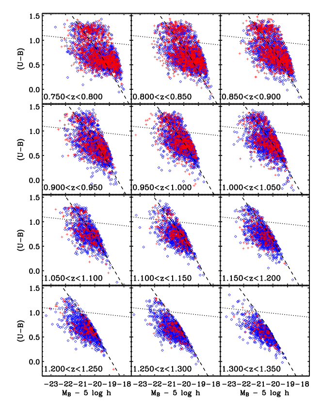
Figure 2: Rest-frame colour-magnitude diagrams for DEEP2 galaxies in redshift bins of width $\delta z=0.05$. Crosses (red) denote galaxies in groups, and diamonds (blue) show field galaxies. Groups that have fewer than two members above the magnitude limit have not been excluded from the group sample in this plot, although they are excluded elsewhere in the paper, as discussed in the text. The dashed lines show the effective DEEP2 apparent magnitude limit, as given in Equation 4.1, using parameters from Table LABEL:tab:samples for $z_{\mathrm{lim}}=1.3$. Dotted lines indicate the division between blue and red galaxies as given in Equation 5.

However, to examine the evolution of galaxy properties, all that is required is to select a region of colour-magnitude space that is uniformly sampled by the survey at all redshifts of interest. Such a selection cut is shown by the dashed curves in each panel of Figure 2, which are described by the equation

$$M_{\mathrm{cut}}-5\log{h} = Q(z-z_{\mathrm{lim}})$$

$$+ \mathrm{min}\left\{[a(U-B)+b],\ [c(U-B)+d]\right\},$$

where $z_{\mathrm{lim}}$ (equal to $1.3$ in the figure) is the limiting redshift beyond which the selected sample becomes incomplete, $a,b,c$, and $d$ are constants that depend on $z_{\mathrm{lim}}$ and are determined by inspection of the colour-magnitude diagrams, and $Q$ is a constant that allows for linear redshift evolution of the typical galaxy luminosity $L^{\ast}$, as already mentioned in § 3. Faber et al. (2006) have measured the evolution of the galaxy luminosity function using data from COMBO-17 (Bell et al., 2004b) and DEEP2 at $z\sim 1$ in conjunction with low-$z$ data from the 2dFGRS (Madgwick et al., 2002; Norberg et al., 2002) and SDSS (Bell et al., 2003; Blanton et al., 2003); they find that changes in $L^{\ast}$ are well described by a linear evolution model, $L^{\ast}\propto Qz$, with $Q=-1.37$. By including this evolution in our selection cut, we are selecting a similar population of galaxies with respect to $L^{\ast}$ at all redshifts.

We use Equation 4.1 to define three different samples, called samples II, III and IV, which are complete in colour-magnitude space to $z=1.0,1.15$ and $1.3$, respectively; the parameters defining these samples are given in Table LABEL:tab:samples. In addition, we create a sample, called sample I, that is purely absolute-magnitude-limited (relative to $M^{\ast}$) and complete to $z=1.0$ by applying a simple cut at $M_{B}-5\log{h}=-20.7+Q(z-1.0)$. Table LABEL:tab:samples summarizes the properties of the resulting samples, and Figure 3 shows colour-magnitude and colour-redshift diagrams for the galaxies in each sample. These samples should also be useful for future studies of colour evolution in DEEP2.

Selecting galaxy samples according to Equation 4.1, effectively creates a sample that is volume-limited for each colour. That is, the selection is colour-dependent, but the magnitude limit relative to $M^{\ast}$ is redshift-independent. This selection is different than the traditional volume-limited selection, but it nevertheless allows for comparison of the relative numbers of galaxies of different colours at different redshifts; that is, it allows us to examine the evolution of the blue fraction. It should be noted, however, that our values of $f_{b}$ cannot be meaningfully compared to published values at low redshift, which have typically been computed using a simple magnitude cut. In particular, our values of $f_{b}$ will be much higher than local values from the literature since the magnitude cut in Equation 4.1 selects many more blue galaxies than red. Indeed, $f_{b}$ values cannot even be compared among the different samples defined in Table LABEL:tab:samples. The absolute values of $f_{b}$ in each sample are mainly set by the selection; useful information comes only from splitting these samples into subsamples to look for trends with redshift or with galaxy properties.

Before we move on, it is important to note that the application of our colour-magnitude selection criteria has important implications for the definitions of our group and field samples. The VDM group catalogue has been defined using the entire apparent-magnitude-limited survey. It is thus possible that a group could have been detected with two or more members at $z=0.8$, say, while only one of these members is brigher than $M_{\mathrm{cut}}$. Had this group instead been at $z=1.3$, it clearly would not have been identified, and its one bright galaxy would have been considered to lie in the field. If no correction is made for this effect, the application of $M_{\mathrm{cut}}$ will cause a redshift nonuniformity in our samples, with galaxies from relatively faint groups being counted as group members at low $z$ and as field members at high $z$. To avoid such biases, we redefine the group sample to be only those galaxies that reside in groups with two or more members brighter than $M_{\mathrm{cut}}$. The field sample comprises all other galaxies.

We also define a group’s richness $N$ to be the number of galaxies with $M_{B}\leq M_{\mathrm{cut}}$ instead of the total number of observed galaxies, so that richness is measured consistently at all $z$ (other group properties, like $\sigma_{v}$ and mean $z$, are still computed using all observed group members, for the sake of robustness). This group definition ensures that our sample of group galaxies is drawn from comparable groups at all $z$, although it means that a given group may have a different value of $N$ in each sample. Also, throughout this paper we will restrict the group galaxy sample to those galaxies whose host groups have velocity dispersions $\sigma_{v}\geq 100\mathrm{\;km\;s^{-1}}$. This is because, as shown in Gerke et al. (2005) (see Figure 8 of that paper), groups with lower velocity dispersion are predominantly false detections. We therefore class galaxies in such groups with the field sample. This point is discussed further in § 5.1. Figure 4 shows the distribution of groups and their member galaxies as a function of $N$ and $\sigma_{v}$ for each of the four samples.

Table 1: Summary of the data samples

	Sample I	Sample II	Sample III	Sample IV
Description	Simple $M_{B}-M^{\ast}$	Colour-magnitude	Colour-magnitude	Colour-magnitude
	limit to z=1.0	complete to z=1.0	complete to z=1.15	complete to z=1.3
$z_{\mathrm{lim}}$	1.0	1.0	1.15	1.3
$a$	0	-1.34	-1.55	-1.94
$b$	-20.70	-18.55	-18.77	-18.92
$c$	…	-2.08	-2.32	-2.90
$d$	…	-17.75	-18.16	-18.53
# galaxies	2691	9546	11767	12493
# groups	232	863	933	851
# group galaxies	531	2588	2605	2211
overall $f_{b}$	0.603 $\pm$ 0.011	0.827 $\pm$ 0.005	0.877 $\pm$ 0.004	0.924 $\pm$ 0.003
field $f_{b}$	0.624 $\pm$ 0.012	0.854 $\pm$ 0.005	0.893 $\pm$ 0.004	0.933 $\pm$ 0.003
group $f_{b}$	0.517 $\pm$ 0.025	0.749 $\pm$ 0.010	0.818 $\pm$ 0.008	0.876 $\pm$ 0.008

Figure 3: Summary of the galaxy catalogue in each of the four samples defined in Table LABEL:tab:samples. The left-hand panels show colour-magnitude diagrams for the samples, and the right-hand panels show colour-redshift plots. The redshift limits of the samples are apparent, as are the effects of our colour-magnitude selection criteria (Equation 4.1). In the bottom three rows, contour lines are evenly spaced in point density.

Figure 4: Summary of the group catalogues in each of the four samples defined in Table LABEL:tab:samples. Solid lines show the differential distribution of groups as a function of richness (number of galaxies above $M_{\mathrm{cut}}$ for the sample) and velocity dispersion $\sigma_{v}$. Dashed lines show the total numbers of galaxies within those groups that fall in a given bin.

4.2 Correcting for incompleteness

Before we may proceed with measuring $f_{b}$, an additional effect must be accounted for. Because of the finite slit length available on the DEIMOS spectrograph, DEEP2 can target for spectroscopy only $\sim 60\%$ of the galaxies that meet its selection criteria (we will call the remaining potential targets “unobserved galaxies”). Moreover, $\sim 30\%$ of galaxies that are targeted for spectroscopic observation fail to yield redshifts (we will call these “redshift failures”). Follow-up observations have shown that many ($\sim 50\%$) of the redshift failures, especially for blue galaxies, lie at redshifts beyond the range probed by DEEP2 (C. Steidel, private communication). The overall failure rate is also correlated with observed galaxy colour and magnitude, although the trends are only slight. Other failures may occur because of poor observing conditions, data reduction errors (e.g., poor subtraction of night-sky emission), or instrumental effects (e.g., bad CCD pixels), but such problems are only a minor contribution to the overall failure rate. These various sources of incompleteness may introduce spurious evolutionary trends in $f_{b}$ unless an appropriate correction is applied.

In this work we adopt the corrective weighting scheme used by Willmer et al. (2006) in measuring the DEEP2 luminosity function. A method of this sort was first implemented by Lin et al. (1999) for the CNOC2 Redshift survey. We locate each galaxy in the three-dimensional space defined by observed $R$ magnitude and $R-I$ and $B-R$ colours. We then define a cubical bin (0.25 magnitudes on a side) in this space around each galaxy with a successful redshift and compute a weight for the $i$th such galaxy:

$$\chi_{i}=1+\frac{\sum_{j}P_{i}(z_{\mathrm{lo}}\leq z_{j}\leq z_{\mathrm{hi}})}{N_{z}^{i}}.$$ (2)

Here $N_{z}^{i}$ is the number of galaxies in the bin around galaxy $i$ with successful redshifts within the nominal DEEP2 redshift range ($z_{\mathrm{lo}}=0.7\leq z\leq 1.4=z_{\mathrm{hi}}$), $j$ is an index that runs over all galaxies in the bin for which DEEP2 did not successfully measure a redshift (whether they were observed or not), and $P_{i}(z_{\mathrm{lo}}\leq z_{j}\leq z_{\mathrm{hi}})$ denotes the probability that galaxy $j$ (in the bin around galaxy $i$) falls in the nominal DEEP2 redshift range.

To compute the probability $P$ in equation 2, we must construct a model for the redshift distributions of redshift failures and of unobserved galaxies. Modeling this in detail would require additional assumptions, but it is reasonably certain that the truth lies between two extreme models. As noted previously, many of the failures are known to be at $z>1.4$, so we can start by making the extreme assumption that all failures lie in this range. In this case, called the “minimal” model, all redshift failures have $P_{i}(z_{\mathrm{lo}}\leq z_{j}\leq z_{\mathrm{hi}})=0$ in equation 2, and unobserved galaxies have

$$P_{i}(z_{\mathrm{lo}}\leq z_{j}\leq z_{\mathrm{hi}})=\frac{N^{i}_{z}}{N^{i}_{z}+N^{i}_{zl}+N^{i}_{zh}+N^{i}_{f}},$$ (3)

where $N^{i}_{zl}$ is the number of galaxies (in the $i$th bin in colour-colour-magnitude space) with redshifts observed to be below $z_{\mathrm{lo}}$, $N^{i}_{zh}$ is the number with $z>z_{\mathrm{hi}}$, and $N^{i}_{f}$ is the number of observed galaxies that failed to yield a redshift. Taking the opposite extreme, we could assume that redshift failures have exactly the same redshift range as the galaxies with successful redshifts. In this case, called the “average” model, both redshift failures and unobserved galaxies have the same value for $P_{i}$:

$$P_{i}(z_{\mathrm{lo}}\leq z_{j}\leq z_{\mathrm{hi}})=\frac{N^{i}_{z}}{N^{i}_{z}+N^{i}_{zl}+N^{i}_{zh}}.$$ (4)

Since blue galaxies with failed redshifts are known to be frequently beyond the DEEP2 redshift range, Willmer et al. (2006) adopted a compromise model (the “optimal” model), in which blue galaxies (see § 4.3 for the precise definition) are corrected with the minimal model while red galaxies are weighted using the average model. We shall adopt this scheme in what follows; however, our basic conclusions are insensitive to the weighting scheme used and in fact are unchanged even when no weighting is used.

4.3 Computing the blue fraction

Having defined a galaxy sample using equation 4.1 and a set of galaxy weights $\chi_{i}$ using equation 2, we may now compute $f_{b}$ for our chosen sample. As in Willmer et al. (2006) we divide the galaxies into red and blue subsamples according to the observed bimodality in galaxy colours. This division corresponds to the dotted line shown in all panels of Figure 2, given by the equation

$$U-B=-0.032(M_{B}-5\log{h}+21.62)+1.285-0.25,$$ (5)

which was derived from the van Dokkum et al. (2000) colour-magnitude relation for red galaxies in distant clusters. Eqn. 5 shifts that relation downward by 0.25 magnitudes to pass through the valley in the colour distribution, following Willmer et al. (2006). One can also allow this colour division to evolve with redshift according to passive stellar evolution models; however, there is no evidence in the DEEP2 data for any evolution in the position of the valley (See Figure 2), and a realistic amount of evolution has only minimal effects on our results (see §5.2). In the interest of simplicity, therefore, we do not allow the division to evolve in most of what follows. This division between red and blue galaxies produces a set of $M$ blue galaxies out of a total sample of $N$ galaxies, each of which is assigned a weight $\chi_{i}$. The corrected blue fraction is then given by

$$f_{b}=\mathcal{N}_{b}/\mathcal{N}_{t},$$ (6)

where the number of blue galaxies $\mathcal{N}_{b}$ and the total number of galaxies $\mathcal{N}_{t}$ are defined as

$$\mathcal{N}_{b}=\sum_{j=1}^{M}\chi_{j},\;\mathcal{N}_{t}=\sum_{i=1}^{N}\chi_{i}$$ (7)

with the index $j$ running over all of the blue galaxies and the index $i$ running over the full galaxy sample.

4.4 Estimating errors on $f_{b}$

The formal error in $f_{b}$ is given by simple binomial statistics:

$$\sigma^{2}_{\mathrm{bin}}(f_{b})=\frac{\mathcal{N}_{b}(\mathcal{N}_{t}-\mathcal{N}_{b})}{\mathcal{N}_{t}^{3}}$$ (8)

(except in the case $\mathcal{N}_{b}=0$, for which De Propris et al. (2004) argue that $\sigma(f_{b})=1/(2\mathcal{N}_{t})$). However, this formula will not fully account for the scatter in our measured values of $f_{b}$. Because a correlation exists in DEEP2 between local galaxy density and galaxy colour (Cooper et al., 2006b), large-scale structure will induce an intrinsic scatter in values of $f_{b}$ measured over a finite volume, in addition to the formal binomial error; this can be thought of, in essence, as a contribution to the error from cosmic variance. We discuss the effects of this scatter further in § 5.2. Also, errors in the galaxy weights $\chi_{i}$ will add scatter to the measured $f_{b}$ values. We therefore find it most convenient to estimate our errors empirically.

We do this in three different ways to ensure that our methods are robust. First, we compute $f_{b}$ for each of the 10 DEEP2 photometric pointings individually and average those computed values; the error $\sigma(f_{b})$ is then taken to be the standard error on that mean. Second, we estimate $\sigma(f_{b})$ using a jackknife sampling strategy in which each pointing is removed in turn from the full dataset being considered, $f_{b}$ is computed for each subsample, and the error on $f_{b}$ for the full sample is estimated using the usual jackknife error formula. Finally, we compute the errors on $f_{b}$ using a bootstrap resampling strategy in which the entire data subsample under consideration (e.g. all group galaxies in a given redshift bin) is randomly sampled with replacement, and the error on $f_{b}$ is estimated from the standard deviation of the $f_{b}$ distribution for 500 such Monte-Carlo samples, using standard bootstrap methods. In each case, the estimated error must be scaled up by a factor of $1.08$ to account for the covariance that exists between contiguous pointings due to large-scale structure fluctuations (i.e., cosmic variance). This factor is derived from Monte Carlo tests based on the covariance between fields with the actual DEEP2 geometry, using the cosmic variance calculation code of Newman & Davis (2002); it corresponds to the conservative assumption that pointing-to-pointing variations in $f_{b}$ are dominated by cosmic variance.

These three different methods give comparable results, though the standard-error and jackknife estimates are much noisier than those from bootstrapping. In the interest of stability, we will always report the bootstrap error values in what follows. It is, however, worth emphasizing that even this method may not account for all sources of $f_{b}$ variance in a given redshift bin, since the DEEP2 dataset is finite. Because $f_{b}$ seems to be lower in higher-density regions, if we are particularly unlucky and there is a net overdensity or underdensity at a given $z$ in most of the DEEP2 fields, this may lead to a fluctuation in $f_{b}$ that is not accounted for in our error bars. In particular, it appears that there may be an underdensity at $z\sim 0.9$ in most of the DEEP2 fields; this may lead to unusually high values of $f_{b}$ at that redshift. To ameliorate this problem, in addition to computing $f_{b}$ in independent bins, we will also sometimes compute $f_{b}$ in a sliding box, which will smooth out any large-scale structure fluctuations at the expense of introducing bin-to-bin correlations in the resulting measurements.

5 Results

Table LABEL:tab:samples shows the properties of the four samples defined in § 4.1, including blue fractions. A primary result of this work is apparent in the last two rows of the Table: in all four samples considered, the blue fraction is significantly lower in groups than it is in the field. Thus, the well-known qualitative distinction between local field and group (or cluster) galaxy populations was in place by $z\sim 1$. It is, however, worth emphasizing that the quantitative increase in $f_{b}$ values from sample I to sample IV is not evidence for evolution because the overall value of $f_{b}$ in each sample is strongly affected by the sample-selection procedures in § 4.1 (i.e., sample IV has a much more sharply tilted selection cut than sample II, so it will include proportionally fewer red galaxies by construction). In what follows, we will divide each sample into redshift bins, allowing for a meaningful investigation of evolutionary trends in the blue fraction. First, though, it is important to understand the trends that exist at fixed redshift.

5.1 Blue-fraction trends at fixed redshift

As discussed in the introduction, the blue fraction in local clusters exhibits a large system-to-system scatter that arises, at least in part, because the measured value of $f_{b}$ depends on exactly which galaxies and clusters are used to compute it (e.g., De Propris et al. 2004; Poggianti et al. 2006). Before considering $f_{b}$ evolution in DEEP2, then, it is crucial to understand trends in the blue fraction at fixed redshift; otherwise they may introduce selection effects that enhance or compete with evolutionary effects (e.g., Smail et al. 1998). As discussed in § 5.2 below, there is little to no evolution in $f_{b}$ over the redshift range $0.75<z<1.0$ in DEEP2, so we will limit ourselves to this range (i.e. to samples I and II) when studying trends at fixed redshift.

First, it is interesting to consider the effect of galaxy magnitude on the blue fraction. In doing this, it is important to use the same absolute magnitude cuts at all colours (i.e., vertical lines in Figure 2). If one instead used tilted cuts like the ones that define samples II–IV (Equation 4.1), the extreme slopes of these cuts in colour-magnitude space would mean that the brightest magnitude bins would exclude all red galaxies while keeping some blue ones, leading to obviously spurious results. Thus we are limited here to subsamples of sample I, the smallest sample in this study. It is also important to allow the magnitude bins to evolve with redshift in the same manner as $M^{\ast}$, to ensure that similar galaxies are being compared across the redshift range. Thus, we divide sample I into bins in the quantity $M_{B}-5\log{h}+Q(z-1)$, with $Q=-1.37$.

Figure 5, shows $f_{b}$ in bins of absolute magnitude for galaxies in groups and in the field. Groups here are defined to be those systems that have two or more members in sample I. A trend is evident for both populations, with brighter subsamples having a lower blue fraction—except for the brightest galaxies, where the trend may reverse. This last result is consistent with the results of Cooper et al. (2006b), who find a population of bright, blue DEEP2 galaxies in high-density environments; it can possibly be ascribed to AGN and starburst activity. It is also interesting to compare the trends for the fainter group and field populations. Fitting a straight line for each subsample, excluding the brightest bin, yields a slope of $0.102\pm 0.033$ for the field population and $0.106\pm 0.044$ for the group galaxies. That is, there is evidence for a similar trend with limiting magnitude for $f_{b}$, both in groups and in the field. We will discuss the implications of this result in § 7.

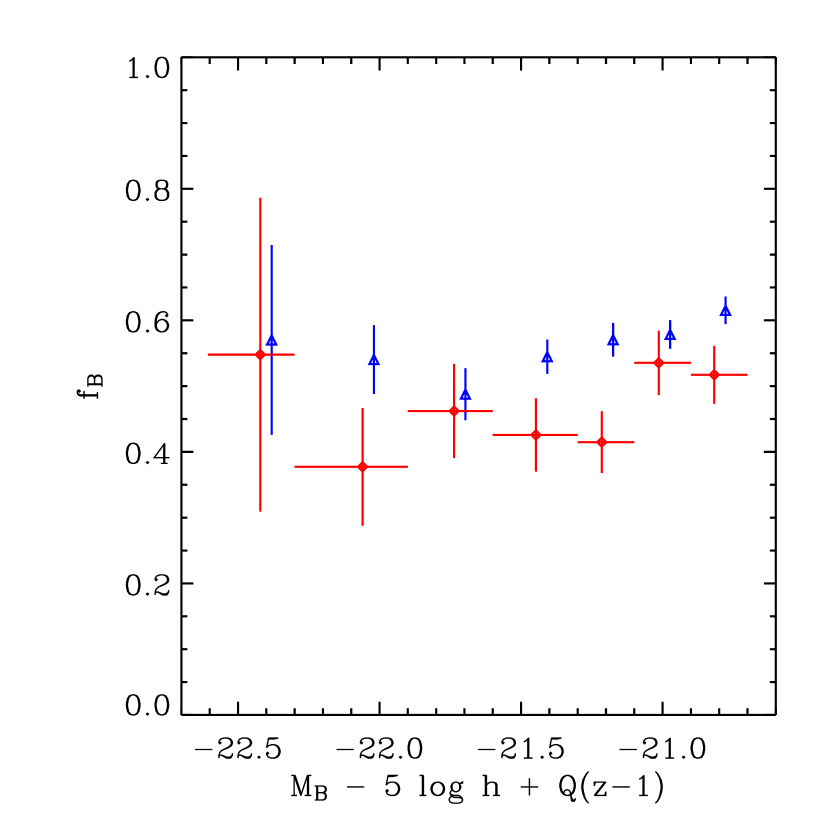
Figure 5: Dependence of the blue fraction $f_{b}$ on absolute magnitude in sample I ($0.75\leq z\leq 1.0$), for galaxies in groups (diamonds with horizontal bars) and in the field (triangles). The data points show $f_{b}$ in bins of evolution corrected absolute magnitude, $M_{B}-5\log{h}+Q(z-1.0)$, where we have adopted the Faber et al. (2006) value of $Q=-1.37$. Horizontal bars (suppressed for the field sample) show the bin size used to compute each data point, and vertical bars show the $1\sigma$ error on $f_{b}$, computed from bootstrap resampling of the galaxies in each bin. Data points have been offset slightly in the horizontal direction for clarity. Groups contain fewer blue galaxies than the field at all magnitudes except possibly in the brightest bin. In addition, a trend is apparent for both group and field galaxies, with brighter galaxies being redder on average, except at the bright end, where the trend may reverse. Linear fits to both trends, excluding the brightest bin, show that their slopes are consistent with the same value.

Figure 6: Dependence of the blue fraction $f_{b}$ of group galaxies in sample II ($0.75\leq z\leq 1.0$) on various group parameters: from upper left to lower right, these are the velocity dispersion of the host group, $\sigma_{v}$; the richness (number of galaxies above the magnitude limit) of the host group; distance from the centre of the host group, in units of $r_{200}$ (see text) and in megaparsecs; and peculiar velocity relative to the host group’s redshift, in units of the host group’s velocity dispersion, and in $\mathrm{\;km\;s^{-1}}$. In each panel, the data points show $f_{b}$ in bins whose sizes vary to ensure robust statistics; the bin sizes are shown by the horizontal bars. As in Figure 5, vertical bars show the $1\sigma$ bootstrap errors.The value of $f_{b}$ for field galaxies is shown as the dotted line. See § 5.1 for details of the selection in each panel and § 4.3 for details of the computation of $f_{b}$.

We will use Sample II to explore other possible systematic trends in $f_{b}$ at fixed $z$, since it is significantly larger than sample I by virtue of the tilted colour-magnitude selection criterion used to define it. Figure 6 shows $f_{b}$ for the group galaxy population only, binnned by various group or galaxy properties. For comparison, the blue fraction for field galaxies is shown as a dotted line. The upper left panel shows the dependence of $f_{b}$ on the velocity dispersion $\sigma_{v}$ of the galaxies’ host groups—that is, each bin contains all of the galaxies in groups with $\sigma_{v}$ in the range of that bin. In this panel, we have included in the group sample those galaxies in groups with $\sigma_{v}<100\mathrm{\;km\;s^{-1}}$, unlike all other plots in this paper. As shown, in terms of $f_{b}$ these galaxies bear a much stronger resemblance to the field than to the rest of the group sample. This is no surprise, since these groups are known to be predominantly false detections—i.e., chance associations of field galaxies (Gerke et al., 2005). Figure 6 then stands as further justification for our decision to class these galaxies with the field. The other data points in this panel show an interesting trend with $\sigma_{v}$: $f_{b}$ declinines with $\sigma_{v}$ at low dispersion and then rises again at high dispersion. Caution is warranted, however, because (1) high dispersion groups are more likely to be contaminated by interloper field galaxies, since the VDM group finder uses a larger search volume for such groups; and (2) the large uncertainty in the measured values of $\sigma_{v}$ for DEEP2 groups makes it difficult to assess the reality of observed trends of galaxy properties with group velocity dispersion. In particular, point (2) might be a problem because the sample has many groups with two members, for which measurements of $\sigma_{v}$ are maximally uncertain. Such groups might dominate over the population of true high-dispersion systems, which are rare. If there were, say, an underlying monotonic decline in $f_{b}$ with increasing $\sigma_{v}$, then the up-scattered small groups could induce an apparent upturn at the high-$\sigma_{v}$ end. For these reasons, we refrain from drawing conclusions regarding the relation between $f_{b}$ and $\sigma_{v}$.

There is, however, an apparent trend with group richness, $N$, at high values of $N$, visible in the top right panel of the figure. Richness in this context is defined to be the number of galaxies in a given group above the colour-magnitude limit $M_{cut}$ that defines sample II (see Equation 4.1 and Table LABEL:tab:samples). The blue fraction declines at the highest richness values. This result illustrates the primary reason that we included in our sample only those groups with two or more members above $M_{cut}$: had we not done so, we would have been sampling richer groups at higher redshifts, potentially causing a spurious decrease in $f_{b}$ with increasing redshift.

The remaining four panels investigate the dependence of $f_{b}$ on group members’ distance from their host groups’ centres (group-centric radius) and on their peculiar velocity relative to their host groups. To probe dependence on group-centric radius, we compute $f_{b}$ for group galaxies within annuli on the sky around the mean right ascension and declination of their host group. The annuli are defined in two ways—in units of comoving Mpc and also in units of $r_{200}$, the radius at which the group is 200 times denser than the background. This radius can be estimated from the group’s radial velocity dispersion $\sigma_{r}$ as

$$r_{200}=\frac{\sqrt{3}\sigma_{r}}{10H(z)},$$ (9)

where $H(z)$ is the redshift-dependent Hubble parameter (Carlberg et al., 1997). We compute each group member’s peculiar velocity with respect to the mean redshift of its host group as $v_{\mathrm{pec}}=c(z-\bar{z})/(1+\bar{z})$, and we consider the peculiar velocity both in units of $\mathrm{\;km\;s^{-1}}$ and normalized to the host group’s velocity dispersion $\sigma_{v}$. The middle two panels of Figure 6 show the dependence of $f_{b}$ in groups on the group-centric distance, and the bottom two panels show the dependence on peculiar velocity. None of these plots shows a significant trend, and linear fits to the data points in each panel are consistent with zero slope.

The lack of a trend with group-centric radius may be surprising in light of studies of groups and clusters at low (e.g., Whitmore et al. 1993; De Propris et al. 2004) and high (e.g., Postman et al. 2005) redshift, showing a strong relation between cluster-centric radius and galaxy type. However, there is a large uncertainty in the determinations of DEEP2 group centres and mean redshifts since these involve taking means of a small number of objects, so it is likely that any trends would be significantly diluted by scatter in these values. Nevertheless, there is a hint in the lower left panel that galaxies at low values of $v_{\mathrm{pec}}/\sigma_{v}$ and $r/r_{200}$ tend to be redder than the general group population. In addition, in the lower right panel it appears that group galaxies with moderate absolute peculiar velocities are redder than usual, while those with the highest velocities are blue. This echoes the trend with $\sigma_{v}$ at upper left (as expected, since only high-$\sigma_{v}$ groups contain galaxies with high values of $v_{\mathrm{pec}}$); these two panels taken together suggest that a negative correlation between $f_{b}$ and $\sigma_{v}$ for DEEP2 groups may be masked by the presence of interloper field galaxies that preferentially lie at high values of $v_{\mathrm{pec}}$. It would be preferable if we could compute Fig. 6 using only high-richness groups, whose dispersions and centers can be determined more robustly; however, restricting even to groups with $N>3$ reduces the sample size so significantly that no firm conclusions can be drawn in light of the resulting error bars. Thus, in the absence of any significant measured trends, we see no justification for further restricting our sample by peculiar velocity or group-centric radius—for instance by taking only galaxies within $r_{200}$ as has been done in various other studies (e.g., De Propris et al. 2004; Poggianti et al. 2006), in which it was possible to measure $r_{200}$ more robustly than it is here. In what follows, the sample of group galaxies will always include all galaxies in groups with $\sigma_{v}>100\mathrm{\;km\;s^{-1}}$ and with two or more members above $M_{\mathrm{cut}}$, regardless of radius or peculiar velocity.

5.2 The evolution of the blue fraction

Having ensured that the group sample will not be affected by trends at fixed redshift that will complicate comparisons at different redshifts, we now proceed to probe the evolution of the blue fraction with $z$. We divide each of the samples in Table LABEL:tab:samples into several independent redshift bins containing equal numbers of galaxies, and we compute $f_{b}$ in each bin for the group and field galaxy subsamples. As discussed in § 4.4, there may be scatter from bin to bin that exceeds the error estimates, especially at $z\sim 0.9$, so to smooth out this effect we also compute $f_{b}$ in a sliding box whose width is twice the average width of the independent bins in each sample.

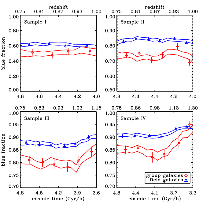
Figure 7: Evolution of the blue fraction with redshift and cosmic time (time since the big bang). For all four samples defined in Table LABEL:tab:samples, the evolution of $f_{b}$ is shown from $z=0.75$ to the limiting redshift of each sample. In each panel, data points show $f_{b}$ values in six independent bins (only four for sample I, which is much smaller than the others) containing equal numbers of galaxies (Note that these bins are typically broader than the ones used in Figure 2; each bin contains a significant number of red galaxies). Blue triangles show $f_{b}$ for field galaxies, and red diamonds denote $f_{b}$ for group galaxies; these points have been slightly offset in the redshift direction for clarity. Lines show 1$\sigma$ errors on $f_{b}$ computed in a sliding bin of twice the mean width of the independent bins. Note that the four panels’ axes have different horizontal and vertical scales; the absence of the upturn at high redshift in the top two panels is owing to the fact that these panels do not extend beyond $z=1$. Over the redshift ranges in common, all samples are fairly consistent. In particular, no sample shows significant evolution in $f_{b}$ over the range $0.75<z<1$, but for $z\ga 1$ (samples III and especially IV), $f_{b}$ evolves substantially, with much stronger evolution in groups than in the field. The group and field samples become nearly indistinguishable at the highest redshifts considered. See § 4.3 for details of the computation of the blue fraction.

The resulting $f_{b}$ values for each sample are shown in Figure 7 as a function of redshift and of cosmic time; this Figure summarizes the principal results of this paper. As noted previously, there is clearly a significant difference in the blue fractions of group and field populations at $z\sim 1$. In addition, in all four samples there is no evidence for evolution in $f_{b}$ over the range $0.75<z<1.0$: group and field populations are consistent with constant $f_{b}$ over this range. However, the bottom two panels of the Figure show that $f_{b}$ evolves dramatically at $z\ga 1.0$, and this evolution is much stronger in groups than it is in the field. In fact, interestingly, the two populations appear to converge in terms of $f_{b}$ at $z\sim 1.3$. It is also notable that the evolution in samples III and IV appears to flatten below $z\sim 1$, in agreement with samples I and II. It is important to emphasize that the bins used in the lower right panel of Figure 7 are broader than those shown in Figure 2, so that each bin contains a substantial number of red galaxies; that is, the convergence of the group and field populations at $z\sim 1.3$ does not result from small-number statistics.

To further assess the robustness of these results, we have investigated the effects of changing our assumptions about the DEEP2 redshift incompleteness modeling and the luminosity evolution of the sample. In each panel of Figure 7, the galaxy weighting scheme used is the “optimal” scheme of Willmer et al. (2006), and the magnitude evolution parameter is set to the value found in Faber et al. (2006), $Q=-1.37$. Changing the weighting scheme to either the average or minimal models of Willmer et al. (2006)—or even using no weights whatsoever—effects no qualitative change in the results shown in Figure 7. Similarly, changing the value of $Q$ by $\pm 0.31$ (the $1\sigma$ uncertainty on this parameter from Faber et al. 2006) has no qualitative effect on the results.

As a further test, we also consider the possibility of evolution in the colour of the “green valley” separating red and blue galaxies in colour-magnitude space. If the colour of the valley changes with time, the $f_{b}$ evolution seen in Figure 7 might simply be the result of passive evolution moving galaxies redward across our (fixed) dividing line (e.g., Andreon et al. 2006). However, the existence of a bimodality in the galaxy colour distribution suggests that the division between red and blue galaxies should be drawn through the valley, as we have drawn it, rather than being tied to the colours of red galaxies alone. Simple inspection of Figure 2 shows no clear evidence for evolution in the locus of this valley. Indeed, if one adopts a model in which red galaxies are continuously being formed from blue ones throughout the redshift range of interest (e.g., the “hybrid” model proposed by Faber et al. (2006)), then one would expect little evolution in the valley’s position. As old red galaxies evolve passively toward redder colours, new red galaxies are formed to take their place, resulting in a red sequence that broadens with time, while the valley between red and blue galaxies remains nearly fixed.

Nevertheless, it is worth exploring the effect of allowing the dividing line to evolve. Blanton (2006) showed that the locus of the green valley has evolved redward by at most $\sim 0.1$ magnitudes in $u-g$ from $z=1$ to the present day. We test the effect of this evolution by applying a colour separation which is given by Equation 5 at $z=1$, with a linear evolution of 0.1 magnitudes redward per unit decrease in redshift (that is, the blue-red dividing line gets redder with time, as might be expected from passive evolution). The evolution of $f_{b}$ with this evolving cut in sample IV is shown in Fig 8. As shown, the evolving colour separation produces a (marginally significant) drop in the group $f_{b}$ from $z=0.75$ to $z=1.0$, probably because the green-valley evolution we assume here is too strong. This is followed by a rise at higher redshifts and a convergence of the group and field values at $z\sim 1.3$. Hence, the main results of Figure 7 still hold: there is substantial evolution in $f_{b}$ in groups at $z\ga 1.0$, with a convergence of the group and field $f_{b}$ values at $z\sim 1.3$.

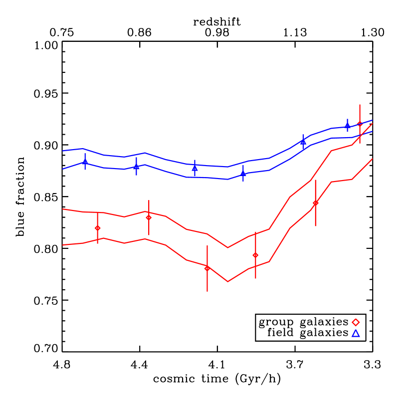
Figure 8: Evolution of $f_{b}$ in sample IV, when the dividing line between red and blue galaxies is allowed to evolve redward by 0.1 magnitudes per unit decrease in $z$ (Blanton, 2006). There is a (probably spurious) drop in $f_{b}$ out to $z=1.0$ (see text), but at higher redshifts the evolution is the same as observed with a non-evolving separation in Figure 7.

Before this result can be fully accepted, however, there is another systematic effect that should be considered. It has been observed (e.g, Bell et al. 2004a; Weiner 2005) that there are two distinct classes of red galaxies at high $z$: nonstar-forming, “red-and-dead” early-types and dust-reddened, star-forming late-types. The latter class will presumably exhibit spectral emission lines; hence it should be relatively easy to obtain redshifts for these galaxies, even if their spectra have low signal-to-noise ratios. Redshifts may be harder to obtain for the nonstar-forming class, since these exhibit weaker spectral features in general. It is thus possible that DEEP2 fails to obtain redshifts preferentially for high-redshift (i.e. faint) early-types. This would mimic evolution in $f_{b}$ both in groups and in the field, but if early-type galaxies occur preferentially in groups, this selection effect could potentially also lead to the convergence seen in the group and field $f_{b}$ values at $z\sim 1.3$. In principle, the weighting scheme described in § 4.2 should approximately correct for this effect; however, if the situation is so dire that all galaxies at a given redshift and in a particular region of colour-colour-magnitude space are redshift failures, then the weighting will be of no help.

This potential bias must therefore be taken seriously. Fortunately, it is possible to get some sense of its importance by looking at the HST/ACS imaging that the AEGIS collaboration has obtained in the EGS (Davis et al., 2006). Supposing that the true mix of spheroidal and dusty-spiral red galaxies in the field is constant with redshift, if early-types are being preferentially missed at high redshift, this would result in a declining ratio of dead to dusty among red field galaxies in DEEP2. We have examined all of the red field galaxies with HST imaging and confirmed DEEP2 redshifts in the range $0.75<z<1.3$ in the EGS (a total of 63 galaxies). At all redshifts, roughly $50\%$ of these show no visible evidence for star formation or spiral structure. Hence, it appears that DEEP2 is not preferentially failing to obtain redshifts for a particular class of red galaxies at high $z$, although it is worth emphasizing that this conclusion has been drawn from a limited sample of galaxies.

The strong evolution of the DEEP2 group blue fraction at $z\ga 1.0$ therefore appears to be robust. It can be explained either by a blue galaxy population that decreases with time, a red galaxy population that increases with time, or both. As shown in Bell et al. (2004b), Willmer et al. (2006) and Faber et al. (2006), there is significant growth in the typical comoving number density $\phi^{\ast}$ of red-sequence galaxies over the redshift range probed by DEEP2, while $\phi^{\ast}$ for blue galaxies has remained roughly constant over this range. Hence, it seems reasonable to ascribe the evolution of $f_{b}$ to the preferential build-up of the red galaxy population in groups. This conclusion is made manifestly clear in Figure 9. Rather than showing fractions, this figure shows the (incompleteness-weighted) numbers of galaxies from sample IV in each of the redshift bins shown in the lower right panel of Figure 7, both in groups and in the field. More specifically, the figure shows the total number of galaxies $\mathcal{N}_{t}$, the number of blue galaxies $\mathcal{N}_{b}$ (see Equation 7), and the number of red galaxies $\mathcal{N}_{r}=\mathcal{N}_{t}-\mathcal{N}_{b}$, all as a function of redshift, both in groups and in the field. It is important to reiterate that the redshift bins were chosen to contain equal unweighted total numbers of galaxies, so the overall weighted numbers in each bin are not constant. In any case, we find that the results of this paper are insensitive to the weighting scheme we choose and remain unchanged even if no weights are applied at all.

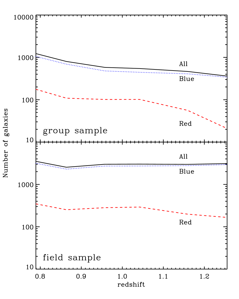
Figure 9: Incompleteness-corrected galaxy counts used to compute $f_{b}$ for sample IV in Figure 7. Solid lines show the total number of galaxies, $\mathcal{N}_{t}$ (see Equation 7), in groups (top) and the field (bottom), for the six redshift bins shown in the bottom right panel of Figure 7. Dotted lines show the number of blue galaxies, $\mathcal{N}_{b}$, in these bins, and dashed lines show the number of red galaxies, $\mathcal{N}_{r}=\mathcal{N}_{t}-\mathcal{N}_{b}$. As shown, while the overall number of group galaxies is growing with time, the number of red galaxies in groups increases much more rapidly, increasing by almost an order of magnitude over the redshift range shown.

The figure shows that $\mathcal{N}_{t}$ for groups increases with time, as expected in the hierarchical $\Lambda$CDM structure-formation paradigm. But $\mathcal{N}_{r}$ in groups grows at a much faster rate, increasing by almost an order of magnitude from $z\sim 1.3$ down to $z\sim 0.75$. At the same time $\mathcal{N}_{t}$ in the field stays nearly constant, and $\mathcal{N}_{r}$ in the field increases only modestly (by a factor of $\la 2$) over this range. It seems clear, then, that the build-up of red sequence galaxies over the DEEP2 redshift range has taken place preferentially within groups and clusters.

6 Tests with mock catalogues

The above results so far appear to be robust, but to establish them definitively it is vital that we also test for biases introduced by the group-finding procedure. For example, it is well known (and has been confirmed here) that groups and clusters are populated by redder galaxies than the field, but, as shown in Figure 2, the DEEP2 apparent magnitude limit selects strongly against red galaxies at high redshift. If red galaxies dominate groups and clusters, this effect might cause their richnesses to appear strongly reduced at high redshift—so much so that they might eventually become undetectable with the VDM group-finder. The high-redshift VDM group sample would then be dominated by false detections. If this were the case, then the group and field populations identified by the VDM would necessarily be indistinguishable, since they would essentially be random subsamples of the same galaxy population, and so the convergence of the group and field populations seen in Figure 7 would simply be the result of group-finding errors and not of genuine galaxy evolution in groups.

We can test for such an effect by running the VDM group-finder on the DEEP2 mock catalogues described in § 3. As discussed in that section, the mock galaxies are assigned rest-frame $U-B$ colours according to the observed DEEP2 colour-magnitude-environment in the redshift range $0.8<z<1.0$. Figure 10 shows the evolution of $f_{b}$ in the mocks for galaxies in real groups (i.e., galaxies that actually reside in dark matter haloes that contain other galaxies, lower curve), for galaxies in found groups (i.e., galaxies in groups identified by the VDM algorithm, diamond points), and for the field samples that complement each group sample (upper curve and triangle points). In computing $f_{b}$, the same limit in colour-magnitude space is applied as the one used for sample IV (given by Equation 4.1 and Table LABEL:tab:samples and shown in Figure 2), and, as in the data, galaxies are included in the group sample only if their host group has two galaxies brigher than the limit. As Figure 10 illustrates, the VDM group-finder reduces the separation in $f_{b}$ between the group and field samples (as expected, since the found groups are contaminated by interloper field galaxies). However, it does not induce a spurious evolutionary trend in the blue fraction of the found group sample: the slopes of $f_{b}$ versus $z$ are consistent for the real and found samples. Thus it does not appear that the VDM group finder is introducing spurious trends in the measurement of blue fraction evolution.

Finally, it is interesting to note in Figure 10 that the values of $f_{b}$ for the true group and field samples in the mocks show clear evolution. As discussed in Section 3, we have not introduced any redshift dependence in the colour-environment relation used to assign colours to mock galaxies. By design, the blue fraction will remain constant with redshift for comparable local density values. Therefore, the evolution of $f_{b}$ seen in the mocks can only be due to evolution in the distribution of local densities within the mocks. That is, the growth of large-scale structure in the mocks causes the number of high-density regions to grow with time, so there are fewer red galaxies at high redshifts in the mocks simply because there are fewer galaxies in overdense environments at high redshifts. This effect provides a partial explanation for the evolution in $f_{b}$ observed in DEEP2. However, because the mock group and field samples remain distinguishable in terms of $f_{b}$ at all redshifts while the observed samples do not, there must also be some decrease in the blue fraction of DEEP2 group galaxies with time at fixed overdensity. (This can also be seen directly in Figure 9, where the numbers of red galaxies in groups grow more rapidly than the total group population.) We will discuss this further in Section 7.

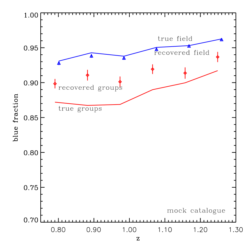
Figure 10: Evolution of the blue fraction in the mock catalogues described in Section 3. Solid lines show the true evolution of $f_{b}$ in the mocks, in groups (lower curve) and in the field (upper curve), computed using real groups, i.e., sets of galaxies that actually occupy common dark matter haloes. Data points show the reconstructed evolution of $f_{b}$ in the mocks, computed using found groups, i.e., groups of galaxies identified in redshift space by the VDM group-finding algorithm. As expected, the distinction between found groups and the field is smaller than the distinction for real groups because of interlopers; however, it is clear that the group-finder does not induce a reconstructed $f_{b}$ evolution that is stronger than the actual evolution in the mocks or as strong as what is observed in the data.

7 Discussion

The main results of this paper are (1) a significantly lower value of $f_{b}$ in group versus field populations at $z\sim 1$; (2) a strong increase of $f_{b}$ in groups with redshift at $z\ga 1.0$; (3) the lack of any obvious $f_{b}$ evolution, for either groups or the field, at lower redshifts; (3) a convergence of $f_{b}$ for the group and field populations at $z\sim 1.3$; (5) a decline in $f_{b}$ in richer groups; and (6) a negative correlation between $f_{b}$ and galaxy luminosity, both in groups and in the field. In light of Figures 7 and 9, it appears especially clear that the build-up of the DEEP2 red galaxy population has taken place most dramatically in groups and clusters rather than in the field (here and throughout, field refers to all galaxies not in groups).

In interpreting this conclusion, three interrelated questions arise.

1. What physical mechanisms are acting in groups and clusters to quench star formation and produce the evolution seen in § 5.2?

2. Is the evolution of $f_{b}$ in DEEP2 groups and clusters simply an extension of the similar evolution seen at low redshift—i.e., is this just the BO effect at high $z$, or are other mechanisms in effect at this epoch?

3. If groups and clusters are the site of red galaxy formation, what is the nature of the red galaxies present in the field, especially those at high redshift?

By comparing these results to other studies at high and low redshift—and to current theoretical models of galaxy evolution—we can attempt to fit our observations into a coherent picture of star formation and quenching in groups and clusters.

7.1 Comparison to the evolving colour-density relation

As shown in § 5.2, the blue fraction in DEEP2 groups evolves strongly over the range $1.0\la z\la 1.3$, and the group and field populations become indistinguishable in terms of $f_{b}$ at $z\sim 1.3$. These results are qualitatively consistent with recent work studying the evolution of the high-redshift galaxy population as a function of local galaxy density, both in DEEP2 and in other surveys. In a companion paper to this one, Cooper et al. (2006a) show that a correlation exists between galaxy red fraction ($f_{r}=1-f_{b}$) and local overdensity out to $z>1$ but that this correlation vanishes at $z\sim 1.3$, in close agreement with our findings here.

Nuijten et al. (2005) used galaxies in the photometric CFHT Legacy Survey to show that the fractions of red and morphologically early-type galaxies grow with time and evolve more strongly in high-density regions than elsewhere. In addition, Tanaka et al. (2005) compared photometric observations of two high-redshift clusters to the SDSS galaxy population; they find that the color-density relation has steepened with time and that this steepening is strongest in very overdense regions. However, as shown in Cooper et al. (2005), photometrically determined redshifts are not sufficient for accurate determinations of galaxy density. Also, Nuijten et al. (2005) consider galaxies above a set of fixed absolute magnitude limits rather than allowing their limits to evolve as $M^{\ast}$. Since galaxies that are faint relative to $M^{\ast}$ tend to be bluer than average (see Figure 5), and because $M^{\ast}$ is brighter back in time, a fixed cut in $M$ includes more faint (blue) galaxies at high redshift, which causes $f_{b}$ to increase (spuriously) with z. This selection effect acts to enhance the observed evolution.

Also, Cucciati et al. (2006) recently considered the fractions of galaxies in various colour ranges as a function of redshift and local density in the VVDS redshift survey. They find that the density dependence of the blue and red fractions vanishes at $z\sim 1.0$, a somewhat lower redshift than we find (see Cooper et al. 2006a for a detailed discussion). They also find that the blue fraction falls with time at all densities, in contrast to our finding that $f_{b}$ is roughly constant in the field at all redshifts. We see are two possible reasons for this (minor) disagreement: first, these authors again consider only a fixed absolute magnitude limit rather than taking $M^{\ast}$ evolution into account, and second, as they also caution, their faint, red galaxy sample is incomplete at the highest redshifts they consider, so any evolution of $f_{b}$ in this range will be spurious. In this paper, we have been careful to design galaxy samples that avoid such subtle selection effects. We are thus able to confirm that the results from the three papers above (Nuijten et al., 2005; Tanaka et al., 2005; Cucciati et al., 2006) are qualitatively correct despite possibly suffering from such effects.

We have also considered groups versus the field, rather than local density. This will be useful in that it allows our results to be interpreted in terms of the dark matter haloes hosting DEEP2 galaxies and compared more readily to theory (see Section 7.3). Local density remains a powerful tool for studying galaxy populations, however, since it probes a wider range of environments than groups and clusters, allowing one to explore whether galaxy evolution might be driven by processes that occur on scales larger (or smaller) than the scale of groups and clusters, or whether underdense regions are as important to galaxy evolution as overdense regions. We therefore urge the reader to compare our results to those of Cooper et al. (2006a). In particular, that paper shows that the red fraction of galaxies in overdense regions declines strongly with increasing redshift, while remaining constant in underdense regions, and that the red fractions of these two environments converge at $z\sim 1.3$. This result is strikingly consistent with the lower right panel of Figure 7 and stands as confirmation that the results presented in this paper are correct.

Both the overdensity considerations of Cooper et al. (2006a) and the halo-mass considerations of this paper point to a partial answer to the question of which mechanisms are driving the evolution we observe. As discussed in § 2.2, DEEP2 samples intermediate-mass objects (in the range $5\times 10^{12}\la M/M_{\odot}\la 10^{14}$), rather than rich ($M\sim 10^{15}M_{\odot}$) clusters. Also, Cooper et al. (2006a) find that the relation between galaxy colour and overdensity is a smooth function of overdensity and does not set in only at the highest densities. We may thus confidently conclude that the quenching of star formation in groups and clusters cannot be ascribed solely to processes that are significant only in rich clusters, such as ram-pressure stripping and harassment (similar conclusions have been drawn in lower-redshift studies as well, e.g., Balogh et al. 2002).

7.2 Comparison to the Butcher-Oemler effect

It is nevertheless tempting to identify the $f_{b}$ evolution seen in Figure 7 with a simple extension of the BO effect to higher redshifts. It is difficult, however, to square this interpretation with the weak or nonexistent evolution seen over the range $0.75\leq z\la 1.0$. To be sure, this redshift range might not sample a long enough period of cosmic time to discern evolution due to the BO effect: “classical” detections of the BO effect (e.g., Butcher & Oemler 1984; Rakos & Schombert 1995; Margoniner & de Carvalho 2000; Kodama & Bower 2001) have typically considered clusters over a redshift range $0\la z\la 0.4$, which corresponds to $3h^{-1}$ Gyr of cosmic time, whereas the range $0.75\leq z\leq 1$ covers only $0.8h^{-1}$ Gyr. Nevertheless, at minimum, if the evolution observed here is simply the BO effect extended to high-redshift groups, the evolution becomes substantially more rapid at $z\ga 1.0$.

Moreover, it is not even clear that groups of the sort being considered in this study would be expected to exhibit a strong BO effect at lower redshifts. As shown in Figure 4, the vast majority of DEEP2 groups have velocity dispersions $\sigma_{v}\la 600\mathrm{\;km\;s^{-1}}$. Because most groups also have very few galaxies with spectroscopy (typically fewer than ten), there is also a very large scatter (typically a few hundred $\mathrm{\;km\;s^{-1}}$) in the measured dispersions. Coupled with the fact that the number of groups falls very steeply with increasing $\sigma_{v}$, this scatter implies that the measured dispersions will tend to be biased high by an Eddington-type bias, so that DEEP2 groups are typically not as massive as their velocity dispersions seem to imply. Also, as discussed above, our mock catalogues imply that DEEP2 does not sample high-mass clusters. There have been very few studies of galaxy evolution in the intermediate-mass systems we do sample, but a recent study by Poggianti et al. (2006) has shown that the fraction of [O II] emitting galaxies does not evolve significantly out to $z\sim 0.8$ for groups with $\sigma_{v}\la 500\mathrm{\;km\;s^{-1}}$. Also, in their study of the morphology-density relation at $z\sim 1$, Smith et al. (2005) show that galaxies in intermediate-density environments show little morphological evolution down to the $z\sim 0.5$ epoch studied by Dressler et al. (1997). If we naively identify intermediate-density environments with intermediate-mass groups like the ones in DEEP2, we might also not expect to find significant evolution in $f_{b}$ over the range $0<z\la 1$. Indeed, preliminary indications (Gerke et al. in prep.) are that $f_{b}$ is little different in DEEP2 groups out to $z\sim 1$ than it is in the groups detected by Eke et al. (2004) in the 2dFGRS, at least for the galaxy population considered in sample I (but see Martínez et al. 2006).

In light of the theoretical basis for the BO effect, it is not surprising that the effect would appear weak in the DEEP2 sample. As first discussed by Kauffmann (1995), the BO effect is a natural outcome of hierarchical structure formation so long as cluster environments are efficient at quenching star formation in galaxies. Since clusters form at late times, galaxies in clusters observed at high redshift will have spent less time on average in the cluster environment than their counterparts observed at low redshift. Hence, they will have had less time to feel the effects of the physical mechanisms that are acting to quench star formation. This picture implies that the BO effect will be weaker in less massive systems, as is observed in, e.g. Poggianti et al. (2006), since smaller systems will typically form earlier and then merge into larger systems, resulting a similarly young galaxy population at all redshifts in these objects. Kodama & Bower (2001) considered a set of simple models for the star-formation histories of cluster galaxies, and their results support the basic Kauffmann (1995) scheme: the observed BO effect can be explained by the decreasing accretion rate onto clusters at late times, coupled with a declining star-formation rate in field galaxies. Neither of these studies considered the effect of dark energy on this picture, but it is worth noting that, in the concordance $\Lambda$CDM cosmology, the universe becomes vacuum dominated around $z\sim 0.4$, sharply attenuating matter infall onto clusters at later times. Infall rates should be much higher at the redshifts considered in this paper; hence one might expect a weaker BO effect in DEEP2, since the quenching blue galaxy population in groups and clusters is being steadily replaced by new infalling galaxies.

It therefore seems reasonable to conclude that the evolution seen at $z\ga 1$ in DEEP2 is different in nature from the low-redshift BO effect. This is not to say that the physical mechanisms quenching star formation in individual galaxies are necessarily different at the two epochs; rather, the evolution may simply be in the efficiency with which these mechanisms alter the bulk properties of the cluster galaxy population. In particular, the rapid evolution at $z\ga 1.0$ and the convergence of the group and field $f_{b}$ values at $z\sim 1.3$ suggest a picture in which, at the epochs considered in this paper, groups have only recently become efficient environments for quenching, while the group galaxy population has a similar star-formation rate to the field at earlier times. For example, if the quenching processes in groups cause star formation to end on a time scale $\tau_{Q}\sim 1$ Gyr (which best reproduces the BO effect in Kodama & Bower 2001), then DEEP2 groups in this picture would have begun quenching their member galaxies efficiently only 1 Gyr prior to the earliest epoch considered here, i.e., at a redshift $z\sim 1.7$ (for $h=0.7$).

This basic conclusion (that the quenching mechanism turns on only at $z\la 2$) is consistent with observations of high star-formation rates in massive galaxies at $z\sim 2$ (e.g., (Daddi et al., 2004)). In addition, it is supported by the stellar-population study of Schiavon et al. (2006), which shows that nonstar-forming galaxies in DEEP2 at $z\sim 0.9$ have mean stellar ages of roughly $1.5$ Gyr (indicative of quenching at $z\la 2$) (Schiavon et al., 2006). Moreover Harker et al. (2006) have shown that a relatively simple model of stellar population evolution, in which star formation is turned off starting at $z\sim 2$, can explain the build-up of the red sequence from $z\sim 1$ to $z\sim 0$. The conclusion that DEEP2 groups only started quenching their member galaxies at $z\sim 2$ is also nicely consistent with the emerging theoretical picture of galaxy formation (e.g., Dekel & Birnboim 2006), in which star formation is quenched efficiently only in haloes with masses above $\sim 10^{12}M_{\odot}$ at $z\la 2$. We discuss this last point in more detail in § 7.3 below.

It is reasonable to worry, though, that the contamination of the group population by interloper field galaxies might cause the two populations to appear indistinguishable when, in truth, a tiny difference still exists. Certainly Figure 10 shows that such contamination weakens the observed difference between the two populations (although it does not induce spurious evolutionary trends). However, the tests on mock catalogues in Gerke et al. (2005) show that the sample of DEEP2 galaxies in VDM groups is dominated by galaxies that are truly in groups, so it should be possible to discern all but the tiniest differences between the samples. In addition, recall that Cooper et al. (2006a) find a similar convergence in the red fraction of galaxies in the most underdense and most overdense environments. Since that study does not suffer from the same contamination effects as the VDM group catalogue, we may be confident that the apparent convergence of the two populations’ blue fractions cannot be ascribed solely to interloper contamination.

7.3 Comparison to semi-analytic models of galaxy formation

It will be instructive to briefly compare the basic picture that the observations in § 5 imply—namely, that groups are not efficient at quenching star formation at $z\sim 2$—with the picture that emerges from semi-analytic models (SAMs) of galaxy formation. This comparison is especially worthwhile because most SAMs have been designed to reproduce the details of the galaxy population at $z\sim 0$, so comparisons to the high-$z$ DEEP2 population will provide sharp tests of their correctness. We will limit ourselves here to qualitative descriptions and arguments, however, and defer detailed comparisons to future work.

In making the comparison, we will sometimes use as a concrete example the model used by Croton et al. (2006) to populate the Millenium run (Springel et al., 2005), a very large, high-resolution N-body simulation of cosmic structure formation. The elements of this model are qualitatively very similar to other recent SAMs (Bower, 2006; Cattaneo et al., 2006; Kang et al., 2006), all of which have been successful at reproducing the observed luminosity functions and colour distributions of galaxies at $z\sim 0$. In the Croton et al. (2006) model, dark matter haloes are populated with two types of galaxy (Springel et al., 2001): each halo contains one central galaxy and may also incorporate satellite galaxies, whose parent haloes merged with the main halo at some time in the past (this conceptual division of the galaxy population is nearly universal in modern-day SAMs). Each halo is also assumed to contain a baryonic component consistent with the overall cosmic baryon fraction. This gas can fuel ongoing star formation if it cools and is accreted by the halo’s central galaxy (e.g., White & Rees 1978; White & Frenk 1991); hence, in order to cease star formation and permanently join the red sequence, a galaxy must stop accreting new cold gas onto its disk.

Most SAMs admit two basic routes by which gas accretion can be stopped, associated with the two types of galaxy in the halo. In the case of satellite galaxies, their parent haloes’ gas is simply added to the gas reservoir of the larger halo when they are accreted. Gas is then only allowed to accrete onto its central galaxy (which sits at the minimum of the potential well), so model satellite galaxies will cease star formation forever once they have exhausted the gas supply in their discs. All satellite galaxies will thus eventually migrate to the red sequence via strangulation. For central galaxies, the situation is somewhat more complicated. In all haloes, infalling gas is shock-heated to the halo viral temperature, but, in low-mass haloes, that hot gas cools on very short timescales so that accretion onto the central galaxy is very rapid. Star formation never ceases permanently in such galaxies. In more massive haloes, the cooling time is longer, and the gas forms a quasi-static, hot halo of gas. The seperation of haloes into these two regimes—the “rapid cooling” and “static hot halo” regimes—has a long history (e.g., Rees & Ostriker 1977; Blumenthal et al. 1984); recent simulations show that the regimes are divided by a rather sharp transition mass of $\sim 3\times 10^{11}M_{\odot}$ (Birnboim & Dekel, 2003; Kereš et al., 2004).

Regardless of the halo mass, however, hot gas near the centre can still cool, accrete onto the central object, and form stars, unless some other source of energy is available to stop the cooling; this is the well-known cooling-flow problem. Croton et al. (2006) propose to solve this problem via heating from low-luminosity AGN lurking in the haloes’ massive central galaxies. They refer to this heating as “radio mode” AGN feedback, to distinguish it from winds created by bright AGN in the “quasar mode” (which should only temporarily eliminate cold gas from a galaxy). In essence, if the central supermassive black hole (SMBH) is massive enough, its average AGN energy output will be sufficient to offset cooling in the halo gas and stanch the flow of gas onto the central galaxy; this basic idea has also been implemented in other SAMs (Bower, 2006; Cattaneo et al., 2006; Kang et al., 2006). Since halo mass and SMBH mass are linked (e.g., Häring & Rix 2004), this model effectively predicts a threshold mass above which accretion onto the central galaxy ceases; then, once the galaxy has exhausted its existing supply of cold gas, star formation ends.

The threshold mass above which “radio mode” heating can stop cooling flows is a few times $10^{12}M_{\odot}$ (Dekel & Birnboim 2006; Cattaneo et al. 2006; Croton et al. in prep.), roughly an order of magnitude smaller than the typical masses of DEEP2 groups. Thus, the Croton et al. picture implies that all galaxies in DEEP2 groups should eventually be quenched and join the red sequence. The only group members that will be blue (i.e., star-forming or recently star-forming) in that model will be those that recently fell in to their host group and have not yet exhausted the cold gas in their discs. If this picture is accurate, then the convergence of $f_{b}$ for the group and field populations shown in Figure 7 implies that a typical DEEP2 group member at $z=1.3$ was not in a halo above the quenching mass until $\tau_{Q}\sim 1$ Gyr before that epoch. This is broadly consistent with hierarchical structure growth in a $\Lambda$CDM universe. In the Millenium Run, for example, one can trace the history of a typical DEEP2-group-like halo, with a mass of $\sim 10^{13}M_{\odot}$ at $z=1.3$. On average, such a halo’s most massive progenitor at $z\sim 2$ had a mass of $\sim 5\times 10^{12}M_{\odot}$—roughly the mass at which radio-mode heating becomes efficient. There are $1.1h^{-1}$ Gyr of cosmic time between $z=2$ and $z=1.3$, a reasonable timescale for quenching and migration to the red sequence. It is worth pointing out that this explanation is conceptually quite different than the BO effect: as we have used the phrase in this paper, the BO effect is simply a consequence of the assumption that groups and clusters quench star formation (and thus it affects only infalling satellites) whereas the mechanism described here is the onset of quenching in group-size haloes (which affects central galaxies as well).

As we have seen, evolutionary results fit nicely, in a broad sense, with the current semi-analytic picture of galaxy formation. However, there are some difficulties in detail, especially as regards satellite galaxies. Satellites in the model are unable to accrete new gas; such accretion is reserved for central galaxies, regardless of the parent-halo mass. Under these assumptions, groups at $z\sim 1.3$ should have a lower blue fraction than the field, unless all of their galaxies were isolated at $z\ga 2$. Since this seems unlikely, it may be necessary to revise the assumption that all satellites are stripped of their halo gas with equal efficiency, regardless of host-halo mass. Indeed, there is already significant evidence that this is an oversimplification. The Croton et al. (2006) model significantly over-predicts the abundance of faint red galaxies (see their Figure 11). Also, there is evidence that a satellite galaxy’s colour is correlated with the colour of its central galaxy (Weinmann et al., 2006a); this would not occur if all satellites were stripped of their gas with equal efficiency. Most recently, Weinmann et al. (2006b) showed that the Croton et al. model severely underpredicts the blue fraction of SDSS satellites and argued that the efficiency with which gas is stripped from satellite galaxies must scale with the mass of the host halo. We note in passing that such a revision to the model would also account naturally for the correlation seen in Figure 6 between $f_{b}$ and group richness, since more massive groups would quench star formation more efficiently.

7.4 On the nature of the red field galaxies

We close this section by commenting on the continued presence of a significant red galaxy population in the field at high redshift, even when the group and field blue fractions have converged. One of our main conclusions in this work is that groups are the primary locus of quenching and red-galaxy formation, and the most naive interpretation of this statement would suggest that there should be no red galaxies in the field. This is an oversimplification, of course, not only because isolated ellipticals are known to exist locally (e.g., Colbert et al. 2001), but also since the red sequence will be contaminated by some fraction of dusty star-forming galaxies (e.g. Bell et al. 2004a; Weiner 2005). One might also expect such galaxies to be more common at high redshift, when the average star-formation rate of the Universe was higher. It should therefore come as no surprise that DEEP2 contains a non-negligible population of red field galaxies at all $z$, but it is not immediately clear whether dusty star-formers can account for all such galaxies.

To address this issue, we make use of the HST/ACS imaging that has been obtained for a portion the Extended Groth Strip subregion of the DEEP2 survey (Davis et al., 2006). In this region there are eleven red field galaxies in the redshift range $1.15<z<1.3$. Five of these show spiral structure or other visible evidence of star-forming activity, while six appear to be nonstar-forming spheroidal or lenticular objects. Thus it appears that a significant population of early-type field galaxies remains at these redshifts; the red field population observed in DEEP2 cannot be fully accounted for by dusty star-formers.

The issue is further complicated by group-finding errors. The VDM group-finder fails to identify some fraction of group members; these will appear in the field sample, and some of them will be early-types. However, the statistics given in  Gerke et al. (2005) imply that only $11\%$ of the field galaxies identified in sample IV are actually group members (not the value of $6\%$ quoted in § 2.2, since we reclassified a significant number of group galaxies as field galaxies in § 4). As shown in Table LABEL:tab:samples, $12\%$ of these—or $1.3\%$ of the total field sample—will be red. Combining this with the observed fraction of dusty star-formers still does not account for the full population of red field galaxies (about $7\%$ of the field in sample IV).

It is therefore worth considering a few mechanisms by which bona fide early-type galaxies could enter the field population. Here the distinction between central and satellite galaxies will again be useful. The threshold mass for quenching in central galaxies, a few times $10^{12}M_{\odot}$, is somewhat lower than the mass range of groups considered in this study; therefore, there should be a population of quenched central galaxies that do not have satellites that enter the DEEP2 sample; these would appear as red galaxies in the field. This picture naturally leads to the correlation between $f_{b}$ and limiting magnitude seen in Figure 5. The strength of this correlation appears to be the same both in groups and in the field. But if all galaxies above a given mass are quenched, and if halo mass correlates roughly with luminosity, then brighter subsets of the galaxy population will naturally have lower blue fractions, both in groups and in the field. This explanation also fits nicely with the recent results of Conroy et al. (2006), who show that the brightest galaxies’ mass-to-light ratios have grown dramatically between $z=1$ and the present day while $M/L$ has remained roughly constant for fainter galaxies—presumably because the brightest galaxies have ceased star formation but continue to accrete new, non-luminous mass.

In addition, it has been shown that winds from merger-driven quasar activity may expel cold gas from galactic disks (Springel et al., 2005; Hopkins et al., 2005). If such a wind arises in a galaxy whose halo is less massive than the threshold at which “radio-mode” AGN feedback is important, then the galaxy should eventually reincorporate some of the expelled gas and resume star formation. But if the timescale for reincorporation is longer than the lifetime of hot, blue stars ($\sim 1$ Gyr), then such galaxies will temporarily join the red sequence. Such temporarily red galaxies could also account for some red field objects.

It is also noteworthy that the blue fraction in the field appears to evolve at $z\ga 1$, if less strongly than in groups. This can be seen in the lower right panel of Figure 7: $f_{b}$ in the field changes by $\sim 0.05$ between $z=1.0$ and $z=1.3$, while the group value changes by $\sim 0.1$. It is worth exploring whether this effect is real, or whether it can simply be attributed to contamination of the field sample by group galaxies, arising from group-finding errors. Let us assume, to start, that the true blue fraction in the field is constant with $z$. Then, if the field sample contains a fraction $c_{f}$ of contaminating group galaxies, and the group sample similarly has a contamination fraction $c_{g}$ of field galaxies, it is straightforward to show that, for a given observed change $\Delta f_{b}^{\mathrm{group}}$ in the group blue fraction, the observed change in the field blue fraction is

$$\Delta f_{b}^{\mathrm{field}}=\frac{c_{f}}{1-c_{g}}\Delta f_{b}^{\mathrm{group}}.$$ (10)

For sample IV, the success statistics given in Gerke et al. (2005) imply that $c_{g}=0.46$ and $c_{f}=0.11$ (as discussed earlier in this Section). Thus, the observed change in the field blue fraction should be $\sim 20$% of the observed change in the group blue fraction. This ratio is, in fact, marginally consistent with the error bars in Figure 7. Hence, the observed decline in the field blue fraction with time is largely caused by contamination by misclassified group galaxies. This conclusion is supported by the findings of Cooper et al. (2006a), who observe no evolution in the red fraction of galaxies in the most underdense environments. On the basis of the present study alone, however, it remains possible that there is also some small amount of intrinsic evolution in the field population. Such evolution would not be too surprising: since the characteristic halo mass $M^{\ast}$ does not reach the quenching mass of a few times $10^{12}M_{\odot}$ until $z\sim 1$ (e.g., Reed et al. 2003), the number density of quenched central galaxies in the field will be growing relatively rapidly at earlier times. Regardless, it remains clear from Figures 7 and 9 that the build-up of the red sequence in DEEP2 takes place preferentially in groups.

8 Conclusion

We have used the DEEP2 group catalogue of Gerke et al. (2005) to study the blue fraction of galaxies in groups and the field at $z\sim 1$. After creating four samples that are carefully designed to be free from colour-dependent and redshift-dependent selection effects, we probe the dependence of $f_{b}$ on a galaxy’s environment (group or field), on galaxy luminosity, on group properties, and on redshift.

First, over the redshift range $0.75\leq z<1$, there is a significant difference in $f_{b}$ between the DEEP2 group and field populations, with a substantially lower $f_{b}$ in groups than in the field. The well-known colour segregation observed between nearby group and field galaxy populations is thus already in place at $z\sim 1$. In addition, there is a negative correlation between $f_{b}$ and group richness over this redshift range, echoing local correlations between galaxy colour and various proxies for halo mass. A trend also exists at these redshifts between $f_{b}$ and the luminosity of the galaxies being considered, with fainter galaxies being more likely to be blue; the strength of this trend does not appear to depend on whether those galaxies are in groups or the field.

No siginificant evolution in $f_{b}$ occurs in the DEEP2 group or field galaxy populations over the range $0.75\leq z\la 1$; however, at $z\ga 1$, there is dramatic, statistically significant evolution in the group population, with $f_{b}$ rising rapidly as $z$ increases. Most notably, the value of $f_{b}$ in groups becomes indistinguishable from the field value at $z\sim 1.3$. To assess the robustness of these results, we have constructed mock catalogues that replicate the colour-environment correlations in the DEEP2 data. Tests with these mock catalogues indicate that the evolution and convergence are not artifacts of the group-finding algorithm. Moreover, these tests suggest that the observed evolution can be explained partially—but not entirely—by evolution in the distribution of galaxy environments, i.e. by the growth of large-scale structure, coupled with the known correlation between environment and galaxy properties. However, to explain the strong evolution and convergence, some further mechanism is required.

Because the $f_{b}$ evolution appears to weaken at $z\la 1$, we conclude that it is different in nature from the classical BO effect, in which $f_{b}$ in clusters rises dramatically from $z=0$ out to $z\sim 0.5$. Indeed, the BO effect is a natural outcome of hierarchical structure formation, provided that groups and clusters are already efficient at quenching star formation in the galaxies that fall into them. But there is a convergence between $f_{b}$ values in groups and in the field at $z\sim 1.3$, which implies that DEEP2 groups were, at some epoch, not especially efficient at quenching infalling galaxies. In particular, if it takes $\sim 1$ Gyr for a quenched galaxy to join the red sequence, our results indicate that the groups in this study only became suitable environments for quenching at $z\sim 2$.

This conclusion is broadly consistent with current semi-analytic models of galaxy formation (Croton et al., 2006; Bower, 2006; Cattaneo et al., 2006; Kang et al., 2006). In those models, the central galaxies of dark matter haloes are quenched when low-level AGN feedback becomes strong enough to stop gas in the halo from cooling and condensing onto the galaxy to form stars; this process becomes efficient at a threshold halo mass of a few times $10^{12}M_{\odot}$ (Dekel & Birnboim 2006; Cattaneo et al. 2006; Croton et al in prep.). Our mock catalogues imply that the groups observed in DEEP2 have masses in the range $5\times 10^{12}M_{\odot}\la M\la 5\times 10^{13}M_{\odot}$. A typical halo in this mass range at $z\sim 1.3$ will drop below the threshold mass for quenching $\sim 1h^{-1}$ Gyr earlier, at $z\sim 2$. This is a potential explanation for the convergence in the group and field $f_{b}$ values at $z\sim 1.3$. Present-day SAMs may have difficulty explaining these observations in detail, however, particularly because they universally assume that satellite galaxies are quenched in all haloes regardless of mass or redshift. In the future, it will be worthwhile to make detailed comparisons between our observations and the precise predictions of SAMs, in order to refine the physical description of galaxy formation that they provide.

References

- Allington-Smith et al. (1993) Allington-Smith J. R., et al., 1993, ApJ, 404, 521
- Andreon (2006) Andreon S., 2006, MNRAS, 369, 969
- Andreon et al. (2006) Andreon S., et al., 2006, MNRAS, 365, 915
- Andreon & Ettiori (1999) Andreon S., Ettiori S., 1999, ApJ, 516, 647
- Balogh et al. (2002) Balogh M., et al., 2002, MNRAS, 337, 256
- Balogh et al. (2004) Balogh M., et al., 2004, MNRAS, 348, 1355
- Baugh et al. (1996) Baugh C. M., Cole S., Frenk C. S., 1996, MNRAS, 283, 1361
- Bell et al. (2003) Bell E. F., et al., 2003, ApJS, 149, 289
- Bell et al. (2004a) Bell E. F., et al., 2004a, ApJ, 600, L11
- Bell et al. (2004b) Bell E. F., et al., 2004b, ApJ, 608, 752
- Benson et al. (2001) Benson A. J., et al., 2001, MNRAS, 327, 1041
- Birnboim & Dekel (2003) Birnboim Y., Dekel A., 2003, MNRAS, 345, 349
- Blanton (2006) Blanton M. R., 2006, ApJ, 648, 268
- Blanton et al. (2006) Blanton M. R., Berlind A. A., Hogg D. W., 2006, ApJ, submitted (astro-ph/0608353)
- Blanton et al. (2003) Blanton M. R., et al., 2003, ApJ, 592, 819
- Blumenthal et al. (1984) Blumenthal G. R., Faber S. M., Primack J. R., Rees M. J., 1984, Nature, 311, 517
- Bower (2006) Bower R. G., 2006, MNRAS, 370, 645
- Butcher & Oemler (1984) Butcher H., Oemler A., 1984, ApJ, 285, 426
- Carlberg et al. (1997) Carlberg R. G., Yee H. K. C., Ellingson E., 1997, ApJ, 478, 462
- Cattaneo et al. (2006) Cattaneo A., et al., 2006, MNRAS, 370, 1651
- Cavaliere et al. (1992) Cavaliere A., Colafrancesco S., Menci N., 1992, ApJ, 392, 41
- Coil et al. (2004a) Coil A. L., et al., 2004a, ApJ, 617, 765
- Coil et al. (2004b) Coil A. L., et al., 2004b, ApJ, 609, 525
- Coil et al. (2006) Coil A. L., et al., 2006, ApJ, 638, 668
- Colbert et al. (2001) Colbert J. W., Mulchaey J. S., Zabludoff A. I., 2001, AJ, 121, 808
- Conroy et al. (2006) Conroy C., et al., 2006, ApJ, submitted (astro-ph/0607204)
- Cooper et al. (2005) Cooper M. C., et al., 2005, ApJ, 634, 833
- Cooper et al. (2006a) Cooper M. C., et al., 2006a, MNRAS, this volume (astro-ph/0607512)
- Cooper et al. (2006b) Cooper M. C., et al., 2006b, MNRAS, p. 642
- Couch et al. (1998) Couch W. J., et al., 1998, ApJ, 497, 188
- Croton et al. (2006) Croton D. J., et al., 2006, MNRAS, 365, 11
- Cucciati et al. (2006) Cucciati O., et al., 2006, A&A, 458, 39
- Daddi et al. (2004) Daddi E., et al., 2004, ApJ, 600, L127
- Davis et al. (2006) Davis M., et al., 2006, ApJ, in press (astro-ph/0607355)
- Davis et al. (2004) Davis M., Gerke B. F., Newman J. A., 2004, astro-ph/0408344
- De Propris et al. (2004) De Propris R., et al., 2004, MNRAS, 351, 125
- Dekel & Birnboim (2006) Dekel A., Birnboim Y., 2006, MNRAS, 368, 2
- Diaferio et al. (2001) Diaferio A., et al., 2001, MNRAS, 323, 999
- Dressler (1980) Dressler A., 1980, ApJ, 236, 351
- Dressler et al. (1997) Dressler A., et al., 1997, ApJ, 490, 577
- Eke et al. (2004) Eke V. R., et al., 2004, MNRAS, 348, 866
- Ellingson et al. (2001) Ellingson E., et al., 2001, ApJ, 547, 609
- Faber et al. (2006) Faber S. M., et al., 2006, ApJ, submitted (astro-ph/0506044)
- Fairley et al. (2002) Fairley B. W., et al., 2002, MNRAS, 330, 755
- Fasano et al. (2000) Fasano G., et al., 2000, ApJ, 542, 673
- Gerke et al. (2005) Gerke B. F., et al., 2005, ApJ, 625, 6
- Goto (2005a) Goto T., 2005a, MNRAS, 356, 6
- Goto (2005b) Goto T., 2005b, MNRAS, 359, 141
- Goto et al. (2003) Goto T., et al., 2003, PASJ, 55, 739
- Goto et al. (2004) Goto T., Yagi M., Tanaka M., Okamura S., 2004, MNRAS, 348, 515
- Gunn & Gott (1972) Gunn J. E., Gott J. R., 1972, ApJ, 176, 1
- Häring & Rix (2004) Häring N., Rix H.-W., 2004, ApJ, 604, L89
- Harker et al. (2006) Harker J. J., et al., 2006, ApJ, 647, L103
- Hogg et al. (2004) Hogg D. W., et al., 2004, ApJ, 601, L29
- Homeier et al. (2005) Homeier N. L., et al., 2005, ApJ, 621, 651
- Hopkins et al. (2005) Hopkins P. F., et al., 2005, ApJ, 630, 705
- Kang et al. (2006) Kang X., Jing Y. P., Silk J., 2006, ApJ, 648, 820
- Kauffmann (1995) Kauffmann G., 1995, MNRAS, 274, 153
- Kereš et al. (2004) Kereš D., et al., 2004, MNRAS, 363, 2
- Kodama & Bower (2001) Kodama T., Bower R. G., 2001, MNRAS, 321, 18
- Koo (1981) Koo D. C., 1981, ApJ, 251, L75
- Koo (1988) Koo D. C., 1988, in Towards understanding galaxies at large redshift; Proceedings of the Fifth Workshop of the Advanced School of Astronomy, Erice, Italy, June 1-10, 1987 (A89-12501 02-90) Comments on the reality of the butcher-oemler effect. Kluwer Academic Publishers, Dordrecht, p. 275
- Larson et al. (1980) Larson R. B., Tinsley B. M., Caldwell C. N., 1980, ApJ, 237, 692
- Lin et al. (1999) Lin H., et al., 1999, ApJ, 518, 533
- Lubin et al. (2002) Lubin L. M., Oke J. B., Postman M., 2002, AJ, 124, 1905
- Madgwick et al. (2002) Madgwick D. S., et al., 2002, MNRAS, 333, 133
- Margoniner & de Carvalho (2000) Margoniner V. E., de Carvalho R. R., 2000, AJ, 119, 1562
- Margoniner et al. (2001) Margoniner V. E., et al., 2001, ApJL, 548, 143
- Marinoni et al. (2002) Marinoni C., Davis M., Newman J. A., Coil A. L., 2002, ApJ, 580, 122
- Martínez et al. (2002) Martínez H. J., et al., 2002, MNRAS, 333, 31
- Martínez et al. (2006) Martínez H. J., O’Mill A. L., Lambas D. G., 2006, MNRAS, 372, 253
- Metevier et al. (2000) Metevier A. J., Romer A. K., Ulmer M. P., 2000, AJ, 119, 1090
- Miller et al. (2005) Miller C. J., et al., 2005, AJ, 130, 968
- Moore et al. (1996) Moore B., et al., 1996, Nature, 379, 613
- Newberry et al. (1988) Newberry M. V., Kirshner R. P., Boroson T. A., 1988, ApJ, 335, 629
- Newman & Davis (2002) Newman J. A., Davis M., 2002, ApJ, 564, 567
- Norberg et al. (2002) Norberg P., et al., 2002, MNRAS, 336, 907
- Nuijten et al. (2005) Nuijten M. J. H. M., et al., 2005, ApJ, 626, L77
- Oemler et al. (1997) Oemler A., Dressler A., Butcher H. R., 1997, ApJ, 474, 561
- Peacock et al. (2001) Peacock J. A., et al., 2001, Nature, 410, 169
- Poggianti et al. (2006) Poggianti B. M., et al., 2006, ApJ, 642, 188
- Postman et al. (2005) Postman M., et al., 2005, ApJ, 623, 721
- Postman & Geller (1984) Postman M., Geller M. J., 1984, ApJ, 281, 95
- Quintero et al. (2006) Quintero A. D., et al., 2006, ApJ, submitted (astro-ph/0512004)
- Rakos & Schombert (1995) Rakos K. D., Schombert J. M., 1995, ApJ, 439, 47
- Reed et al. (2003) Reed D., et al., 2003, MNRAS, 346, 565
- Rees & Ostriker (1977) Rees M. J., Ostriker J. P., 1977, MNRAS, 179, 541
- Schiavon et al. (2006) Schiavon R. P., et al., 2006, ApJ, submitted (astro-ph/0602248)
- Schlegel et al. (1998) Schlegel D. J., Finkbeiner D. P., Davis M., 1998, ApJ, 500, 525
- Smail et al. (1998) Smail I., et al., 1998, MNRAS, 293, 124
- Smith et al. (2005) Smith G. P., et al., 2005, ApJ, 620, 78
- Spitzer & Baade (1951) Spitzer L., Baade W., 1951, ApJ, 115, 413
- Springel et al. (2005) Springel V., Di Matteo T., Hernquist L., 2005, MNRAS, 361, 776
- Springel et al. (2001) Springel V., et al., 2001, MNRAS, 328, 726
- Springel et al. (2005) Springel V., et al., 2005, Nature, 435, 629
- Szapudi & Szalay (1996) Szapudi I., Szalay A. S., 1996, ApJ, 459, 504
- Tanaka et al. (2005) Tanaka M., et al., 2005, MNRAS, 362, 268
- Toomre & Toomre (1972) Toomre A., Toomre J., 1972, ApJ, 178, 623
- Tovmassian et al. (2005) Tovmassian H. M., Plionis M., Andernach H., 2005, ApJ, 617, L111
- van Dokkum et al. (2000) van Dokkum P. G., et al., 2000, ApJ, 541, 95
- Weiner (2005) Weiner B. J., 2005, ApJ, 620, 595
- Weinmann et al. (2006a) Weinmann S. M., et al., 2006a, MNRAS, 366, 2
- Weinmann et al. (2006b) Weinmann S. M., et al., 2006b, MNRAS, 372, 1161
- White & Frenk (1991) White S. D. M., Frenk C. S., 1991, ApJ, 379, 52
- White & Rees (1978) White S. D. M., Rees M. J., 1978, MNRAS, 183, 341
- Whitmore et al. (1993) Whitmore B. C., Gilmore D. M., Jones C., 1993, ApJ, 407, 489
- Willmer et al. (2006) Willmer C. N. A., et al., 2006, ApJ, 647, 853
- Wilman et al. (2005) Wilman D. J., et al., 2005, MNRAS, 358, 88
- Yan et al. (2006) Yan R., et al., 2006, ApJ
- Yan et al. (2003) Yan R., White M., Coil A. L., 2003, ApJ, 607, 739
- Yang et al. (2003) Yang X., Mo H. J., van den Bosch F. C., 2003, MNRAS, 339, 1057
- Zabludoff & Mulchaey (1998) Zabludoff A. I., Mulchaey J. S., 1998, ApJ, 496, 39