Constraining Black Hole Spin Via X-ray Spectroscopy

Abstract

We present an analysis of the observed broad iron line feature and putative warm absorber in the long 2001 XMM-Newton observation of the Seyfert-1.2 galaxy MCG–6-30-15. The new kerrdisk model we have designed for simulating line emission from accretion disk systems allows black hole spin to be a free parameter in the fit, enabling the user to formally constrain the angular momentum of a black hole, among other physical parameters of the system. In an important extension of previous work, we derive constraints on the black hole spin in MCG–6-30-15 using a self-consistent model for X-ray reflection from the surface of the accretion disk while simultaneously accounting for absorption by dusty photoionized material along the line of sight (the warm absorber). Even including these complications, the XMM-Newton/EPIC-pn data require extreme relativistic broadening of the X-ray reflection spectrum; assuming no emission from within the radius of marginal stability, we derive a formal constraint on the dimensionless black hole spin parameter of $a=0.989^{+0.009}_{-0.002}$ at $90\%$ confidence. The principal unmodeled effect that can significantly reduce the inferred black hole spin is powerful emission from within the radius of marginal stability. Although significant theoretical developments are required to fully understand this region, we argue that the need for a rapidly spinning black hole is robust to physically plausible levels of emission from within the radius of marginal stability. In particular, we show that a non-rotating black hole is strongly ruled out.

1 Introduction

Accreting black holes are the driving force behind some of the most powerful processes in the universe. The central regions of active galactic nuclei (AGN), in particular, are prodigious sources across the electromagnetic spectrum including the X-ray band. The X-ray continuum (which is accurately approximated by a power-law up to $\sim 100{\rm\thinspace keV}$) is thought to be produced by Comptonization processes in the corona (or base of a jet) surrounding the inner part of the accretion disk. A portion of the X-ray photons produced in the corona irradiate the underlying optically-thick disk, producing the so-called “X-ray reflection” signatures in the observed spectrum (Guilbert & Rees 1988; Lightman & White 1988). These X-ray reflection signatures consist of fluorescent and recombination emission lines sitting on a continuum due to Compton scattering and the summed radiative recombination continua of the excited ions in the photoionized disk surface (George & Fabian 1991; Ross & Fabian 2005). The Fe-K$\alpha$ line is the most prominent of these features due to its energy (at $6.4{\rm\thinspace keV}$ it is visible above the direct power law continuum), and the high astrophysical abundance and fluorescent yield of iron. Additionally, this line is often significantly broadened by both the standard Doppler effect and relativistic processes, the effects of which increase the closer the line is emitted to the event horizon (Fabian et al. 1989; Laor 1991). These relativistic processes include light bending, beaming and gravitational redshifting, all of which result in a greatly elongated and skewed line profile; in particular, the line profile can display an extended low-energy tail primarily resulting from gravitational redshift. The line emission region is sufficiently close to the black hole that frame-dragging effects associated with the black hole spin can be important in determining the line profiles. The broad iron line is therefore a powerful probe of the relativistic effects on the spacetime immediately surrounding the black hole.

The first broad iron line robustly detected and resolved in an AGN was found by the Advanced Satellite for Cosmology and Astrophysics (ASCA) in the Seyfert-1.2 galaxy MCG–6-30-15 (Tanaka et al. 1995; Iwasawa et al. 1996), and since then has been extensively studied with BeppoSAX (Guainazzi et al. 1999), RXTE (Lee et al. 1999, 2000), Chandra (Lee et al. 2002; Young et al. 2005) and XMM-Newton (Wilms et al. 2001; Fabian et al. 2002; Reynolds et al. 2004). All of these results show that the broad iron line feature is consistent with a highly redshifted line from the inner parts of an accretion disk; no alternative hypothesis has yet explained the spectrum of MCG–6-30-15 satisfactorily (Fabian et al. 1995; Reynolds & Wilms 2000; Vaughan & Fabian 2004; Young et al. 2005). Subsequent ASCA, Chandra and XMM-Newton studies have discovered similarly broad iron line profiles in several other Seyferts, such as MCG–5-23-16 (Dewangen, Griffiths & Schurch 2003), NGC 3516 (Turner et al. 2002), Mrk335 (Gondoin et al. 2002), and Mrk766 (Pounds et al. 2003a).

In addition to having a sample of objects that have been observed with robust broad iron lines, it is equally important to have a precise model to use in fitting the data. The two line profiles currently included as standard in the current versions of the commonly used spectral fitting package xspec (Arnaud 1996) are useful as a starting point, but ultimately quite limited in terms of their ability to accurately parameterize the line. The diskline model (Fabian et al. 1989) describes the line profile from a disk around a non-rotating (Schwarzschild) black hole, and, due to the approximations employed, does not include relativistic light bending. Similarly, the laor model (Laor 1991) has important constraints as well: this is a fully-relativistic model, but the dimensionless spin parameter of the black hole is hard-wired at $a=0.998$, the equilibrium spin of a black hole accreting from a Novikov & Thorne (1974) accretion disk. Furthermore, due to the computational realities of the early 1990s, the relativistic transfer functions underlying the laor model are pre-calculated and tabulated, yielding noise (or even gross inaccuracies) in the line profiles produced, especially at very high disk inclination angles. Given these limitations, as well as the high quality of AGN spectra currently being obtained with Chandra and XMM-Newton (and hopefully in the future with the remaining operable instruments aboard Suzaku), it is imperative that X-ray astronomers have access to effective models that are fully relativistic, accurate, and that allow black hole spin to be fit as a free parameter. This latter point is crucial if we are to hope to constrain the spin of astrophysical black holes using broad iron lines and other X-ray reflection signatures.

Three new relativistic line models have recently been developed for this purpose and implemented in a form that can be readily used by X-ray astronomers: the ky suite (Dovčiak et al. 2004) and similar codes by Beckwith & Done (2004) and Čadež & Calvani (2005). These models achieve comparable results for the morphologies of the line profiles, and all offer significant improvements over the diskline and laor results in terms of accuracy and precision over a wider range of physical parameters. Most importantly, these models leave the spin of the black hole as a free parameter, include emission from within the innermost stable circular orbit in the disk, and compute fully relativistic photon transfer functions. In practice, the xspec modules that implement both the ky and Beckwith & Done models use relativistic transfer functions stored in very large (multi-gigabyte) pre-calculated tables. Using these models, both groups conclude that fitting broad iron lines cannot truly constrain the spin of the black hole. Since their models allow emission from any radius of the accretion disk outside of the event horizon, they can produce iron line profiles with arbitrarily redshifted wings even if the underlying black hole spacetime has no spin. One must consider the physicality of this assumption, however: it is not possible to get line emission from radii deep within the plunging region for several reasons. Firstly, the closer one gets to the event horizon, the smaller the geometrical area of the disk available for emission becomes, while the gravitational redshift affecting any emission from such regions increases correspondingly. Both of these effects would tend to minimize the contribution to the line profile from most of the emission inside the radius of marginal stability. Further, the ionization of the disk material within $\sim 4\,r_{\rm g}$ of a Schwarzchild black hole is inevitably too high to produce significant line emission in the first place, and the optical depth of this material also decreases rapidly within the radius of marginal stability (Reynolds & Begelman 1997; Young et al. 1998). For all of these reasons, one simply cannot produce significant line emission from any arbitrary radius outside the event horizon. This must be taken into account when modeling such line emission.

In this paper, we undertake a rigorous re-analysis of the broad iron line seen in the $\sim 350{\rm\thinspace ks}$ July-2001 XMM-Newton observation (Fabian et al. 2002). We assess the constraints on the iron line profile and black hole spin including the complications introduced by other spectral components displayed by this system, especially the substantial column of absorbing photoionized gas seen along the line of sight to the central disk of this AGN. To facilitate this investigation, we present a new variable-spin accretion disk line profile model, kerrdisk, that we are currently developing for public use in the xspec package. The principal difference between kerrdisk and the previously mentioned variable-spin line profile models is that our model does not rely on gigabyte-sized, precomputed tables of the photon transfer function over many thousands of radii within the disk. Rather, as we will discuss below, we use the approach of Cunningham (1975) to decompose the line profile integral into a simple analytic component (describing the effects of relativistic beaming) and an additional transfer function (describing the effects of light bending) which is a slowly varying function of black hole spin and disk inclination angle and hence only needs to be coarsely tabulated. This technique allows us to obtain high-quality line profiles with very modest sized (40 MB) tables, making it substantially more portable and convenient than some other models. This accuracy, portability and comparative speed of computation make kerrdisk a valuable addition to the X-ray astronomer’s software arsenal. Additionally, a trivial change of the driver code allows the user to implement any desired limb-darkening law or compute the line profiles to arbitrary resolution and accuracy (if, for example, the user is interested in the narrow cusps of the line profile). Neither of these modifications is possible if the limb-darkening and resolution are hard-wired into the tabulated relativistic transfer functions.

In §2, we motivate our study by giving a brief recap of the history of the broad iron line in MCG–6-30-15. §3 describes our new iron line model, including a detailed comparison of kerrdisk to the other line profile models already discussed. §4 presents our analysis of MCG–6-30-15 using these variable-spin line models. This work is performed under the “standard” assumption that there is no observable X-ray reflection from inside the radius of marginal stability of the accretion disk. A future paper will extend the analysis to the more general case where physically reasonable levels of emission from this region are allowed. Under this assumption we arrive at the conclusion that the black hole in MCG–6-30-15 is a rapid-rotator. §5 and §6 discuss our results and draw conclusions, respectively.

2 A Brief History of Broad Iron Line Studies in MCG–6-30-15

MCG–6-30-15 is an S0-type galaxy in the constellation of Centaurus that hosts a Seyfert-1.2 nucleus. It has a measured redshift of $z=0.008$, placing it at a distance of $d\approx 37{\rm\thinspace Mpc}$ using WMAP cosmological parameters. X-ray studies of this AGN have revealed a powerful central source along with a significantly broadened Fe-K$\alpha$ feature. This broad line has led MCG–6-30-15 to become one of the most studied AGN in the X-ray band due to its potential as a probe of black hole and accretion disk physics. Although the mass of the hole is not yet well constrained, estimates based on X-ray studies have placed it in the range of $10^{6}-2\times 10^{7}\hbox{$\rm\thinspace M_{\odot}$}$ (Nowak & Chiang 2000; Reynolds 2000). McHardy et al. (2005) have further narrowed this mass range to $3-6\times 10^{6}\hbox{$\rm\thinspace M_{\odot}$}$ using a variety of methods such as the M-$\sigma$ relation, line widths from optical spectra, BLR photoionization arguments and X-ray variability.

Reflection signatures from neutral material had been observed with EXOSAT (Nandra et al. 1989) and Ginga (Nandra, Pounds & Stewart 1990; Matsuoka et al. 1990), but it was not until deep observations of MCG–6-30-15 by ASCA that the broadened and skewed iron line was robustly detected (Tanaka et al. 1995). It was determined that the line profile matched that expected due to X-ray reflection from the surface of a relativistic accretion disk; the robustness of this interpretation was demonstrated in Fabian et al. (1995). Broad-band BeppoSAX data taken by Guainazzi et al. (1999) confirmed the Tanaka et al. detection of a broadened and redshifted iron line with an equivalent width of ${\rm EW}\approx 200{\rm\thinspace eV}$.

A detailed re-analysis of this observation by Iwasawa et al. (1996) identified a period of time when the source entered the so-called “deep minimum” state, marked by low continuum emission. While in this state, the iron line width (and especially the extent of the red-wing of the line) markedly increased to the point that emission from a disk around a Schwarzschild black hole truncated at the radius of marginal stability ($r_{\rm ms}=6\,r_{\rm g}$) could no longer reproduce the observed line profile. Noting that the radius of marginal stability moves inwards (to a location characterized by higher gravitational redshift) as the black hole spin is increased, it was subsequently argued that the black hole in MCG–6-30-15 must be rapidly rotating. Fitting sequences of Novikov & Thorne (1974) models to the deep minimum ASCA data (and assuming that the X-ray irradiation tracks the local dissipation in the underlying disk), Dabrowski et al. (1997) derived a lower limit of $a>0.94$ on the rotation of the black hole. At this point, however, Reynolds & Begelman (1997) noted that physically plausible scenarios could result in sufficient X-ray reprocessing (including ionized iron line emission) from within the radius of marginal stability to fit the ASCA deep minimum state with even a Schwarzschild black hole. In order to illuminate the region of the disk within $r_{\rm ms}$, they hypothesized an X-ray source on the symmetry axis some height above the disk, and suggested that iron line profile changes (and some part of the X-ray continuum flux changes) could be attributed simply to changes in the height of this X-ray source.

After the discovery of its broad iron line feature, MCG–6-30-15 became the subject of many more observations. With the first observations of XMM-Newton in 2000, astronomers had a new tool with unparalleled throughput with which to examine this source in finer detail. The first XMM-Newton observation of MCG–6-30-15 was fortunate enough to catch the source in its “deep minimum” state characterized by low continuum flux and a broader than normal Fe-K$\alpha$ profile. The resulting high signal-to-noise spectrum revealed an extremely extended red-wing to the line profile extending down to $3-4{\rm\thinspace keV}$ (Wilms et al. 2001). Because so much emission seemed to be coming from radii deep within the gravitational potential well, and because the emissivity index was correspondingly quite high, the authors hypothesized an interaction between the spinning black hole and its accretion disk. Magnetic torquing effects between the two could result in the extraction of rotational energy from the black hole which would, in turn, power the high coronal emission seen from the inner radii of the disk (Agol & Krolik 2000; Garofalo & Reynolds 2005). An alternative mechanism consists of the strong gravitational focusing of a high-latitude source above a rapidly rotating black hole (Martocchia & Matt 1996; Miniutti & Fabian 2004). By contrast with the ASCA era, a Schwarzschild model appeared not to work for these data — a line extending down to $\sim 3{\rm\thinspace keV}$ would require line emission from extremely deep within the plunge region: $r\approx 3\,r_{\rm g}=0.5\,r_{\rm ms}$, a situation which appears unphysical due to the high ionization expected in this part of the flow (Reynolds & Begelman 1997).

Reynolds et al. (2004) performed a follow-up and more detailed analysis of the XMM-Newton observation of MCG–6-30-15 taken by Wilms et al. (2001). They explicitly demonstrated that the iron line profile was inconsistent with an X-ray irradiation profile that follows a Novikov & Thorne (1974) dissipation law, even for an extremal Kerr black hole. Employing the generalized thin disk model of Agol & Krolik (2000) that includes a torque applied at $r=r_{\rm ms}$, Reynolds et al. (2004) suggested that this torque has a great impact on the disk emission seen in this observation. In the “deep minimum” state, the torqued-disk scenario requires that the disk is largely emitting via the extraction of rotational energy from the black hole rather than via accretion. These authors also examine spectral variability during the deep minimum state. By examining difference spectra and direct spectral fits to $10{\rm\thinspace ks}$ segments of data from this observation, the authors concluded that the intensity of the broad line seems to be proportional to the hard $2-10{\rm\thinspace keV}$ flux of the source: the equivalent width of the line remains approximately constant while the source fluctuates substantially in amplitude. Such behavior is consistent with simple X-ray reflection models.

The longest XMM-Newton observations of the source to date was published by Fabian et al. (2002). This group found MCG–6-30-15 in its normal state, and recorded data for over $87$ hours. In this state, the bulk of the iron line emission was in a narrower line compared with the “deep minimum” state, although a very extended red-wing was still evident. The time-averaged EPIC-pn spectrum again showed that the Fe-K$\alpha$ feature was very strong, and the long data set was of sufficient resolution and quality that the spectrum demanded a fit incorporating a full reflection model. Relativistic smearing needed to be applied not just to the cold iron line, but to the entire reflection continuum. Taking this into account, the iron line was once again found to produce emission within the radius of marginal stability for a Schwarzchild black hole. Fitting the line with the maximally spinning ($a=0.998$) black hole laor model suggested that the line emissivity followed a $\epsilon\propto r^{-\alpha}$ dependence with $\alpha=4.5-6$ between an inner radius $r_{\rm min}<2\,r_{\rm g}$ and a break radius $r_{\rm br}\approx 6\,r_{\rm g}$. Beyond the break radius, the emissivity profile flattened to $\alpha\sim 2.5$. This broken power-law form was strongly preferred by the data over the usual simple power-law emissivity functions usually fitted to such data — again, this reflects the high quality of the data. Fabian et al. (2002) also note that, in its normal state, difference spectra of MCG–6-30-15 show spectral variability from $2-10{\rm\thinspace keV}$ in the form of a power-law: the iron line flux changed little between successive $10{\rm\thinspace ks}$ frames of the observation, whereas the continuum flux varied by as much as a factor of $\sim 2$. This result is in contrast to that found by Reynolds et al. (2004), who observed an iron line flux proportional to the $2-10{\rm\thinspace keV}$ continuum flux when MCG–6-30-15 was in its “deep minimum” state. Comparing these two studies, it appears that the iron line flux is proportional to the observed X-ray power-law continuum at low fluxes and then “saturates” to an approximately constant level once the observed X-ray continuum exceeds a certain level. This complexity could be due to light-bending effects if the power-law X-ray continuum source is situated close to the spin axis of the black hole (Miniutti & Fabian 2004). Alternatively, patchy ionization of the disk surface might produce such a saturation (Reynolds 2000).

Dovčiak et al. (2004) utilize their ky suite of iron line profile models to fit the time-averaged spectrum of MCG–6-30-15 as well, also using data from the long XMM-Newton observation of Fabian et al. (2002). They fit the $3-10{\rm\thinspace keV}$ spectrum with four combinations of ky models, all involving a broad Fe-K$\alpha$ kyrline, a narrow Gaussian emission line at $6.9{\rm\thinspace keV}$ (likely an ionized line of iron, as cited in Fabian et al. (2002)), and a Compton-reflection continuum from a relativistic disk (smeared using a kyconv kernel). The authors also find that models describing the disk emissivity as a broken power-law rather than a single power-law in radius achieve significantly better statistical fits, though among these broken power-law models, comparable fits can be obtained for a wide variety of black hole spin values. These authors therefore conclude that iron line profiles are not a good way to constrain black hole spin. At some level, this objection amounts to obvious point that arbitrarily large redshifts can be obtained around any black hole (rotating or not) if one is at liberty to produce emission from any radius arbitrarily close to the event horizon. One must, however, consider the physical realism of this assumption in general, and the best-fit spectral parameters determined by these authors in particular. For their low-spin ($a=0.25$) best-fitting model, Dovčiak et al. concluded that a substantial amount of iron line emission had to originate from deep within the radius of marginal stability; translating the fit parameters of Dovčiak et al. into standard quantities, they require an inner emissivity profile of $\epsilon\propto r^{-9}$ starting at an inner radius of $r_{\rm in}=3.2\,GM/c^{2}$, to be compared with the radius of marginal stability for a $a=0.25$ black hole which is at $r_{\rm ms}\approx 5.2\,GM/c^{2}$. As has already been noted and will be explored further in §4, it is hard to understand how this region of the accretion flow could contribute to any part of the observed iron emission given that the fact it will be very tenuous and extremely highly photoionized (Reynolds & Begelman 1997; Young, Ross & Fabian 1998).

The medium resolution (CCD) data discussed so far leave ambiguous the possible role of complex ionized absorption in distorting the observed X-ray continuum shape and hence the inferred iron line profile. To assess the role of this absorption, Young et al. (2005) performed and analyzed a deep, $522{\rm\thinspace ks}$ grating observation of MCG–6-30-15 in May-2004 with the HETGS instrument on Chandra. This observation produced two important results: first, the authors found that the difference in the hard continuum spectrum between the high and low flux states was well described by a power-law of photon index $\Gamma=2.0^{+0.2}_{-0.1}$. This finding agreed with previous studies that indicated that the spectral variability of MCG–6-30-15 in its normal state is dominated by a power-law component (e.g. Fabian et al. 2002). Second, and most importantly, ionized absorption models whose continuum curvature mimics the red-wing of a broad iron line from $3-6{\rm\thinspace keV}$ were ruled out. Such models generically predict strong K$\alpha$ absorption lines of intermediately ionized iron. Young et al. showed that these lines are conclusively absent, falsifying the ionized absorption model and further strengthening the relativistic smearing hypothesis.

3 The kerrdisk Model

3.1 Model Description

As discussed in the introduction, we are motivated to construct an iron line model that allows the spin parameter of the black hole to be a free parameter and is maximally flexible.

Our new relativistic emission line code, kerrdisk, is written in fortran77 so that it can be easily meshed with xspec, and has now been compiled successfully on both Solaris and Linux platforms. The dimensionless spin parameter of the black hole ($a=cJ/GM^{2}$; where $J$ is the angular momentum of a black hole of mass $M$) can take on any value in the range $-1\leq a\leq 1$, where negative values of $a$ correspond to a black hole that is rotating in a retrograde sense relative to the accretion disk. Although, according to the equations of General Relativity, $a$ could have any arbitrary value, the cosmic censorship hypothesis states that naked singularities cannot exist in the universe, so a black hole must be shrouded by an event horizon. This limits the acceptable range of spin parameters to $-1\leq a\leq 1$. For simplicity we consider only prograde spins up to the Thorne (1974) spin-equilibrium limit, i.e., $0\leq a\leq 0.998$.

The limiting value of $a=0.998$ for black hole spins was first discussed by Thorne (1974). Therein, the author contends that if black holes were simply accreting matter their spins would ascend to $a\approx 1$ rather quickly, but because material in the accretion disk radiates, and some of that emitted radiation is swallowed by the hole, a counteracting torque is produced. The origin of this counteracting torque lies in the photon capture cross-section of the hole: black holes have a higher capture cross-section for photons of negative angular momentum (opposite to that of the hole itself) than for photons of positive angular momentum. Thus, the accretion of emitted radiation from the disk results in an overall reduction in the angular momentum of the hole until it reaches a theoretical equilibrium value of $a=0.998$. Recent work on magnetohydrodynamic (MHD) accretion disks suggest that the continued transport of angular momentum from matter within the radius of marginal stability, as well as angular momentum lost from the rotating black hole itself via Blandford-Zjanek like mechanisms (Blandford & Znajek 1977), may lead to a rather lower equilibrium spin (e.g., see the general relativistic MHD simulations of Krolik, Hawley & Hirose (2005)). Equilibrium spins as low as $a\sim 0.90$ are within the realm of possibility.

Following the method of Cunningham (1975), we compute the line profile by employing a relativistic transfer function. For a given black hole spin $a$, disk inclination $i$, the observed accretion disk spectrum can be written as

$$F_{\rm obs}(E_{o})\propto\int\frac{g^{2}}{\sqrt{g^{*}(1-g^{*})}}I(E_{o}/g,\theta_{e},r_{e})\psi(r_{e},g^{*};a,i)\,dg^{*}\,r_{\rm e}dr_{e}.$$ (1)

Here, $I(E,\theta_{e},r_{e})$ is the rest-frame specific intensity of the disk at radius $r_{\rm e}$ and energy $E$ emitted at a angle $\theta_{\rm e}$ to the disk normal, $\psi$ is the Cunningham transfer function which accounts for the effects of light-bending on the observed solid angle from each part of the disk, $g$ is the ratio of the observed to the emitted photon energy ($g=E_{\rm o}/E_{\rm em}$), and ${\it g^{*}}$ is the relative value of $g$ with respect to the redshift extremes obtained from that annulus,

$$g^{*}=\frac{g-g_{\rm min}(r_{\rm e})}{g_{\rm max}(r_{\rm e})-g_{\rm min}(r_{\rm e})}.$$ (2)

This formulation is attractive from the computational point of view; light bending effects are isolated from beaming effects and encoded in the transfer function $\psi(r_{e},g^{*};a,i)$ which is a slowly varying function of its variables. This allows us to perform full computations of the transfer function at a relatively sparse set of points in parameter space, and then use interpolation to accurately determine the transfer function at a general point.

Specializing to the case of a $\delta$-function emission line allows us to eliminate the $g^{*}$ integration from Eqn. (1). Assuming that the surface emissivity of the emission line as a function of emission radius $r_{e}$ and angle $\theta_{e}$ is $f(r_{e},\theta_{e})$, this gives

$$F_{obs}(E_{o})\propto\,\int\limits_{r_{\rm min}}^{r_{\rm max}}\,\frac{g^{3}}{\sqrt{g^{*}(1-g^{*}})}\frac{1}{g_{\rm max}-g_{\rm min}}\,\psi(r_{e},g^{*};a,i)\,f(r_{e},\theta_{e})\,r_{\rm e}dr_{e}.$$ (3)

We use the algorithms of Speith et al. (1995) to compute the transfer function $\psi(r_{e},g^{*};a,i)$ as well as $g_{\rm min}(r_{e})$ and $g_{\rm max}(r_{e})$, thereby allowing us to perform this integration. For a given spin $a$ and inclination $i$, high quality line profiles (and all of the line profiles presented in this paper) are produced using a transfer function computed at 50 radial bins, equally spaced in the variable $1/\sqrt{r_{\rm e}}$, and 20 linearly spaced relative redshift (${\rm g^{*}}$) bins across the line profile at any given radius.

These values were determined via rigorous trial and error to make the best, smoothest possible line profile while keeping computation time to a reasonable length. Increasing either the number of radial or relative redshift bins did not significantly improve the integrity of the line profiles produced. Also, because the transfer function varies quite slowly with radius and relative redshift, greater frequency of sampling was not warranted.

Our choice for the radial spacing corresponds to equal spacing of non-relativistic Keplerian velocities. We then evaluate the line profile integral (Eqn. 3) with a densely spaced logarithmic grid in $r_{\rm e}$, using linear interpolation in $r_{\rm e}$ of the (rather sparsely sampled but slowly varying) transfer function. In practice, we use $5n_{\rm e}$-zones per decade of $r_{\rm e}$ where $n_{\rm e}$ is the number of frequency elements in the output line profile (specified by the response matrix of the data being fit). Experimentation shows that this produces high quality line profiles even at very high resolution (i.e., large $n_{\rm e}$).

The Cunningham transfer function $\psi(r_{e},g^{*};a,i)$ is computed for a $20\times 20$ grid in $(a,i)$-space and is stored in a 40 MB table that is accessed by the driver script for kerrdisk. Again, due to the slowly varying nature of the transfer function, simple linear interpolation to arbitrary spins and inclination angles produces accurate and high quality line profiles.

For all of the models explored in this paper, we follow Fabian et al. (2002) and assume a line emissivity characterized by a broken power-law between some inner radius $r_{\rm min}$ and outer radius $r_{\rm max}$, i.e.,

$$f(r_{e})=\left\{\begin{array}[]{ll}0&r_{e}<r_{\rm min}\\ (r_{\rm e}/r_{\rm br})^{-\alpha_{1}}&r_{\rm min}\leq r_{\rm e}<r_{\rm br}\\ (r_{\rm e}/r_{\rm br})^{-\alpha_{2}}&r_{\rm br}\leq r_{\rm e}<r_{\rm max}\\ 0&r_{\rm e}\geq r_{\rm max}\end{array}\right.$$ (8)

We note that, at present, the publicly available Speith algorithms on which this work is based do not support the proper computation of emission from within the radius of marginal stability, i.e., we are restricted to $r_{\rm min}\geq r_{\rm ms}$. Hence, all kerrdisk line profiles currently assume that the emission profile is truncated within $r=r_{\rm ms}$.

The code takes $\sim 4{\rm\thinspace s}$ to produce a single line profile on a $2{\rm\thinspace GHz}$ processor linux machine. When the model is used to fit data within xspec, several hundreds or thousands of iterations of the code are often needed to get a good fit, resulting in run times on the order of an hour or more. In principle, this run time can be significantly reduced by employing a parallelization scheme when fitting. Such a parallelization scheme is possible to implement in the isis spectral analysis package (Houck 2002) using the PVM module (Michael Nowak and Andy Young, private communication).

The best way to examine the results of the code line profile simulations is to look at how the morphology of the line changes with alterations made in certain important variables. For illustrative purposes, Fig. 1 shows model line profiles with a rest-frame energy of $E=1{\rm\thinspace keV}$. The line profiles shown in this figure have the same parameter settings as those shown in the review by Reynolds & Nowak (2003) to enable easy comparison. The Reynolds & Nowak profiles are also based on the Speith algorithms but sample the transfer function more sparsely and employ a cruder integration technique to evaluate the line profile. The fact that our line profiles agree with, but are much less noisy than the Reynolds & Nowak profiles validates our newer integration/interpolation technique.

Figure 1: Variation of the kerrdisk line profile with (a) disk inclination angle, (b) disk emissivity index, and (c) black hole spin parameter. In each case the range of emission in the disk is from $r=r_{\rm ms}-50\,r_{\rm g}.$ In (a), $a=0.998$, $\alpha=1.5$. In (b), $a=0.5$, $i=40$. In (c), $i=40$, $\alpha=3$.

3.2 Comparison With Other Relativistic Disk Line Models

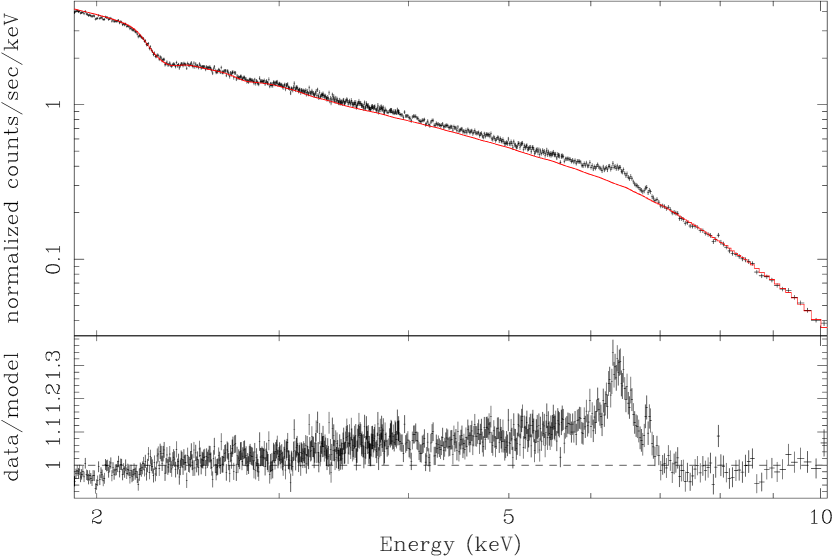
Figure 4: The phabs(po) fit to MCG–6-30-15. Notice the significant deviations of the data from this model, especially around $6.4{\rm\thinspace keV}$. $\chi^{2}/{\rm dof}=4577/1106$ ($4.14$).

Verification of our new line profile code can be demonstrated through detailed comparisons with existing public models, such as laor and diskline (where $a=0.998$ and $0.0$, respectively), as well as those of Dovčiak et al. (2004) and Beckwith & Done (2004). Since the kyrline model of Dovčiak has already been compared with the kdline model of Beckwith & Done (2005), we need only to compare kerrdisk with kyrline. These comparisons are shown in Figs. 2-5 and discussed in this Section.

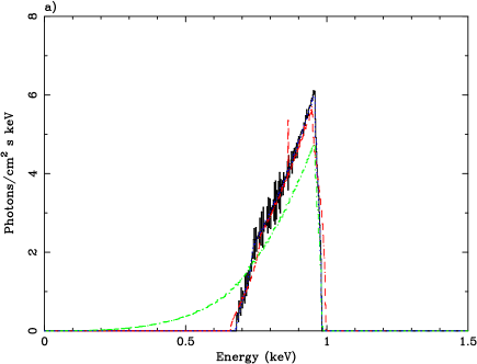
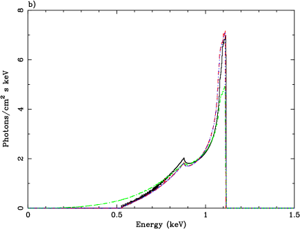
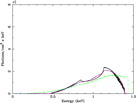
Figure 2: Various iron line models for a Schwarzchild black hole. The inclination angles represented are $5^{\circ}$ for (a), $45^{\circ}$ for (b), and $80^{\circ}$ for (c). Here $\alpha_{1}=\alpha_{2}=3.0$, and $r_{\rm min}$ and $r_{\rm max}$ are held constant at $6\,r_{\rm g}$ and $50\,r_{\rm g}$, respectively. The diskline profile is in solid black, the kerrdisk profile is in dashed red, the kyrline profile including emission from within the ISCO is in dash-dotted green and the kyrline profile not including ISCO radiation is in dotted blue.

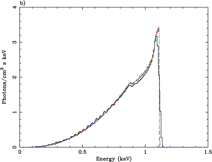
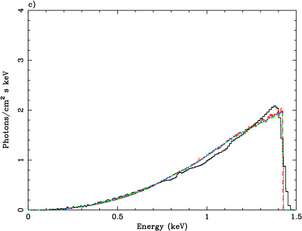
Figure 3: Various iron line models for a maximally spinning Kerr black hole. The inclination angles vary as above for the Schwarzchild case in (a)-(c). Other parameters are the same as those used in the Schwarzchild case, but now $r_{\rm min}=1.235\,r_{\rm g}$, corresponding to the radius of marginal stability for a maximal Kerr black hole, rather than the $6\,r_{\rm g}$ Schwarzchild $r_{\rm ms}$. The laor profile is in solid black and the rest of the color scheme is the same as that used in Fig. 2 above.

Given the lack of relativistic light bending in the diskline model, we expect our (fully relativistic) kerrdisk line profiles with $a=0$ to differ slightly from those computed with diskline, especially at large inclination angles. We indeed see slight differences (Fig. 2). We should stress, however, that the differences are minor and diskline should still be considered a perfectly acceptable model for disks around Schwarzschild black holes for all but the highest signal-to-noise data. Examining the comparison of the laor models with the $a=0.998$ kerrdisk model, we note good agreement (Fig. 3). The slight differences that do exist are caused by an artificial smoothing of the laor line due to interpolation of a sparsely sampled transfer function. Again, however, we note that the laor model is perfectly acceptable model for disks around $a=0.998$ black holes for all but the highest signal-to-noise data.

The real power of this new generation of line profile models is the freedom in the spin parameter of the black hole, therefore the real verification of our code lies in a detailed comparison of kerrdisk and kyrline. Indeed, as shown in Figs. 2-3, the line profiles for kerrdisk and kyrline are virtually indistinguishable when one does not include radiation from within the radius of marginal stability in kyrline. Also shown in these figures are the effects of including emission from within the radius of marginal stability (down to the horizon, for the sake of illustration), as computed by Dovčiak et al. (2004). This has the greatest effect on the line profiles from the slowly spinning holes since it is only in these systems that an appreciable fraction of the plunging region is subject to modest (rather than extremely large) gravitational redshift. We intend to extend our model to include the region within the radius of marginal stability in future work, carefully considering the effects of both the level of ionization and the optical depth of the material within the plunging region, in particular, as discussed in §1. Both of these effects can have a substantial impact on the contribution of emission from this region to the overall line profile.

3.3 The Convolution Model

In reality, the irradiation of the disk by the primary X-ray source results in a whole X-ray reflection spectrum consisting of Compton and radiative recombination continua plus numerous fluorescent and radiative recombination lines. The iron line is the most prominent due to its high rest-frame energy and its intrinsic strength, but many other species are also excited (e.g. oxygen, nitrogen, silicon and sulfur). The whole X-ray reflection spectrum from the disk will be subject to the same extreme Doppler and relativistic processes that combine to alter the morphology of the iron line. The most physically realistic simulation of the reflected spectrum from a photoionized disk surface has been presented by Ross & Fabian (2005) — these high-quality models capture the “traditional” X-ray reflection processes (Compton scattering, photoelectric absorption and fluorescent line emission) as well as the powerful soft X-ray radiative-recombination line emission expected from an X-ray irradiated photoionized surface of an optically-thick accretion disk. Ross & Fabian (2005) have provided their results in the form of tabulated spectra that can be used in xspec. We then wish to convolve this spectrum in velocity space with a relativistic smearing kernel such as the one used to generate the kerrdisk line profile. To facilitate this, we have also produced a convolution form of our line profile model, kerrconv, whose results mirror those of the kyconv model designed by Dovčiak et al. (2004) and the kdconv model of Beckwith & Done (2004), provided that no radiation from within the ISCO is included in the latter two models, as was the case for the comparison of kerrdisk with kyrline and kdline in §3.2 above. As with kerrdisk, the kerrconv parameters include emissivity indices for the inner and outer disk separated by a break radius, inner and outer radii for the disk emission, the spin parameter of the black hole, and the inclination angle of the disk with respect to our line of sight. The kerrconv model is readily validated by applying it to a narrow emission line and comparing the resulting spectrum with the regular kerrdisk model.

4 Determining the Spin of the Black Hole in MCG–6-30-15

In this Section, we use our new models (kerrdisk and kerrconv) along with the model of Dovčiak et al. (2004) to confront the issue of determining the spin of the black hole in MCG–6-30-15. Because of the extremely robust, broad, well-studied iron line in this system, MCG–6-30-15 is an excellent candidate for such a study. Given the complexity of the spectrum displayed by the source, it is important to perform this exercise in a step-by-step manner, clearly enumerating all of the assumptions at each stage, and employing physical models for the spectral complexity whenever possible.

This guides the study presented in this Section. Due to the unprecedented signal-to-noise, we use the EPIC-pn data from the aforementioned long XMM-Newton observation of MCG–6-30-15. Data preparation and reduction followed Vaughan & Fabian (2004) exactly. In this Section, we present a step-by-step analysis of these data using models of increasing complexity and physical realism. Initially, to illustrate the potential power of broad iron lines for spin determination, we modeled the $2-10{\rm\thinspace keV}$ EPIC-pn as a simple power-law continuum modified by a broad iron line (and absorption by the Galactic column of $4.1\times 10^{20}\hbox{${\rm\thinspace cm}^{-2}\,$}$ toward this source); this is comparable to the study performed by Dovčiak et al. (2004). It does, however, neglect the significant effects that continuum curvature due to ionized absorption could have on the inferred iron line parameters (and hence inferred black hole spin). To assess these effects, we next model the effects of multiple warm absorbers and dust on first the $2-10{\rm\thinspace keV}$ spectrum and then the full $0.6-10{\rm\thinspace keV}$ spectrum. In our most sophisticated spectral model, we describe the $0.6-10{\rm\thinspace keV}$ band including multiple absorption components and augmenting the simple broadened iron line with a relativistically smeared ionized X-ray reflection spectrum from Ross & Fabian (2005).

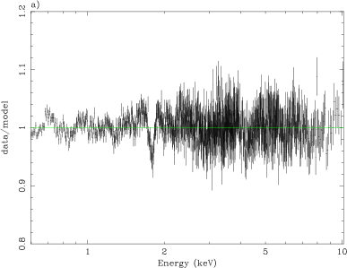
Figure 7: (a) A second warm absorber has been added, as well as an iron edge at $0.707{\rm\thinspace keV}$ and a blackbody component to model direct disk emission. The data now include energies from $0.6-2.0{\rm\thinspace keV}$. The residual feature at $\sim 1.8{\rm\thinspace keV}$ is a calibration artifact (the Si K edge). $\chi^{2}/{\rm dof}=1742/1375$ ($1.27$). (b) $\Delta\chi^{2}$ vs. $a$ plot. At $90\%$ confidence, $a=0.997\pm 0.001$.

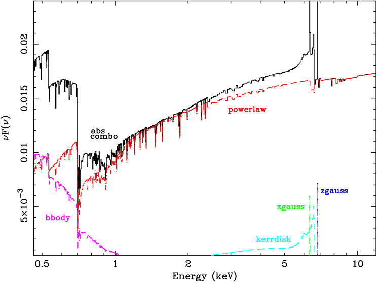
Figure 9: A $\nu F_{\nu}$ plot of the relative contributions of the model components for Model 4, shown above in Fig. 7a. The two redshifted gaussian components (zgauss) are shown in green and dark blue, the kerrdisk line is in light blue, the blackbody component (bbody) representing soft emission from the disk is in purple, and the power-law continuum (powerlaw) is in red. The soft components labeled “abs combo” in black represent the combination of absorption features present in the spectrum: Galactic photoabsorption, two warm absorber models and an iron absorption edge. The solid black line represents the combined model including all the dashed components.

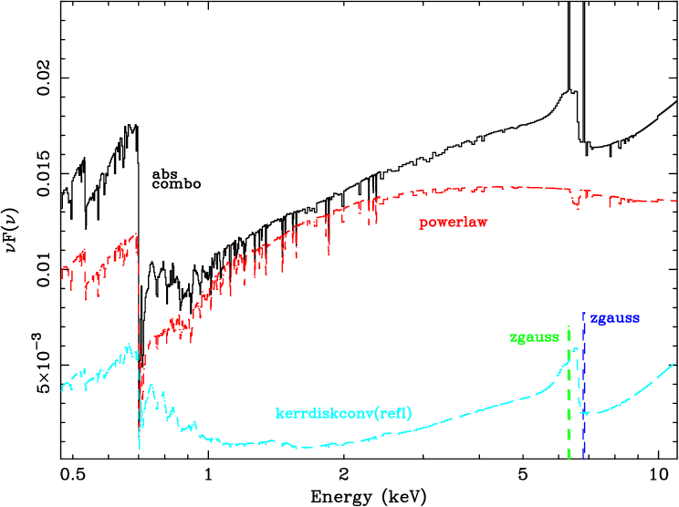
Figure 10: A $\nu F_{\nu}$ plot of the relative contributions of the model components for MCG–6-30-15, as above in Fig. 9. Now the fit is from Model 5, as shown in Fig. 8a. The color scheme is the same as for Fig. 11, but in this case the blackbody component has been replaced by an ionized reflection spectrum to model the soft emission as well as the broad neutral iron line. This component appears in light blue.

The best-fit parameters and error bars for each progressive model fit are shown in Table 1. Each fit and the corresponding $\Delta\chi^{2}$ with respect to changes in $a$ in each case are shown in Figs. 6-10. The unfolded spectrum and the best-fit model components for both the single kerrdisk case and the full ionized reflection spectrum convolved with kyconv are shown in Figs. 11-12. For the warm absorber tables described in Table 1 and §4.2, all abundances are frozen at the solar value. For all model components, the redshift is set to $z=0.008$, the optically determined value for MCG–6-30-15 (Reynolds et al. 1997). In all of the fitting below, the inner disk radius contributing to the iron line emission (or X-ray reflection spectrum in the case of Model 5) was not allowed to be smaller than the radius of marginal stability.

4.1 Simple Power-Law Continuum and Iron Line Across the $2-10{\rm\thinspace keV}$ Spectrum

Initially, we perform an analysis of the $2-10{\rm\thinspace keV}$ spectrum assuming that the underlying continuum is a simple power-law (absorbed by the Galactic hydrogen column) and that the disk spectrum is just a single iron line (rather than a whole reflection spectrum). Fig. 4 shows the hard spectrum as fit by this photoabsorbed power-law (Model 1). To accurately model the continuum we have initially ignored the $4-7{\rm\thinspace keV}$ range when fitting this component. This prevents any contamination of the fit by the presence of an iron line reflection signature. Once the fit was complete, energies from $4-7{\rm\thinspace keV}$ were included again. As suspected, the data/model ratio shown in the lower panel demonstrates a significant residual feature above the continuum, which appears to have the form of a highly broadened iron line peaking at $6.4{\rm\thinspace keV}$. The presence of this large residual feature results in a poor fit, $\chi^{2}/{\rm dof}=4577/1106$. Fig. 5a plots the data/model ratio again, this time for a model including a single, broad kerrdisk line with a rest-frame energy of $6.4{\rm\thinspace keV}$ (Model 2). Two narrow redshifted gaussians representing a cold Fe-K$\alpha$ line and an ionized line of iron are also included at $6.4$ and $6.9{\rm\thinspace keV}$, respectively, as in Fabian et al. (2002). The $6.4$ and $6.9{\rm\thinspace keV}$ lines both have equivalent widths of $\sim 14{\rm\thinspace eV}$.

It should be noted here that Fabian et al. (2002) acknowledged that a $6.74{\rm\thinspace keV}$ absorption line of $EW=-138\pm 35{\rm\thinspace eV}$ fit the data as well as an emission line at $6.9{\rm\thinspace keV}$ and $EW=18\pm 6{\rm\thinspace eV}$. This absorption feature was also preferentially used in the MCG–6-30-15 work of Vaughan & Fabian (2004), and was consistent with the prediction of Sako et al. (2003) based on an RGS observation of this source in 2001. However, the $6.7{\rm\thinspace keV}$ absorption line detected in the deep high-resolution Chandra/HETGS spectrum of Young et al. (2005) is significantly weaker than that fitted by Fabian et al. (2002), with equivalent widths of $EW=-18^{+7}_{-5},-13\pm 9,and-25\pm 9{\rm\thinspace eV}$ during the average, low and high flux states of the source, respectively. Thus, the high-resolution Chandra spectrum does not support a spectral model for the EPIC spectrum in which the complexity in the $6.6-7.0{\rm\thinspace keV}$ range includes a very strong absorption line. Two possible loopholes in this argument are (1) an order of magnitude temporal change in the helium-like iron column density between the XMM-Newton and Chandra grating observations and (2) extreme $\sim 10^{4}\hbox{${\rm\thinspace km}{\rm\thinspace s}^{-1}\,$}$ velocity broadening of the absorption feature which would diminish its detectability in the high-resolution spectrum. More plausible is the notion of a weak ($EW\sim 40{\rm\thinspace eV}$) and slightly broad emission line from hydrogen like iron (Fe xxvi). Given that Chandra shows there to be a weak ($EW\sim-20{\rm\thinspace eV}$) narrow Fe xxvi absorption line at $6.97{\rm\thinspace keV}$, the EPIC-pn spectrum would be expected to show a net emission feature with $EW\sim 20{\rm\thinspace eV}$.

Most importantly, however, the details of whether this spectrum complexity is described by an ionized iron emission or absorption line has almost negligible effect on the broad iron line. In terms of the effect on the overall fit, Fabian et al. (2002) note that the relativistic line parameters differ insignificantly when one employs an absorption line rather than an emission line in the model. We have checked this result in our own analysis; specifically, we have replaced the $6.9{\rm\thinspace keV}$ gaussian in Model 4 with a $6.74{\rm\thinspace keV}$ gaussian in absorption (i.e., negative flux). The result was a $\Delta\chi^{2}/\Delta{\rm dof}=+26/0$, indicating a marginal decrease in the overall goodness of fit. Visually, this fit was indistinguishable from the best fit from Model 4, and as per Fabian et al. , we also found minimal change in the relativistic line parameters. The inner emissivity index of the disk became marginally steeper and its inclination angle increased very slightly, but the changes were well within the statistical error bars. The most interesting point, however, is that the best fit equivalent width of this absorption line was only $-21.3{\rm\thinspace eV}$; much less than the $-138{\rm\thinspace eV}$ found by Fabian et al. . Such a modest equivalent width in comparison to what should be necessary suggests that this line is not robustly wanted in our fit to the data.

The three iron lines (two narrow and one broad) that we do choose to include significantly improve the fit ($\chi^{2}/{\rm dof}=960/1096$), and succeed in modeling out the residual feature shown in Fig. 4. At $90\%$ confidence for one interesting parameter, our best fit for Model 2 indicates a very rapidly rotating black hole ($a=0.970^{+0.003}_{-0.015}$). To gauge the sensitivity of this fit to the spin of the black hole, Fig. 5b plots the change in the goodness of fit parameter $\Delta\chi^{2}$ as a function of black hole spin parameter. This clearly demonstrates that $\chi^{2}$ improves dramatically as one approaches very rapid spins. The equivalent width of the broad iron line in our best-fitting model is $\sim 729{\rm\thinspace eV}$, quite a bit higher than the $\sim 550{\rm\thinspace eV}$ cited by Fabian et al. (2002), the $450{\rm\thinspace eV}$ found by Ballantyne et al. (2003), or the $\sim 250{\rm\thinspace eV}$ found by Dovčiak et al. (2004). This unphysically high equivalent width is clearly due to the simplicity of this model — the effects of absorption and the X-ray reflection continuum, in particular, will introduce additional curvature into the continuum, thereby alleviating the need for such a strong line.

4.2 Modeling the Warm Absorber

In order to accurately assess the width and morphology of the iron line in an AGN, it is imperative that the soft portion of the spectrum be modeled correctly. One must be concerned about confusing a broad red-wing of a relativistic iron line with continuum curvature resulting from a putative “warm absorber” present within the AGN system. In fact, it has been argued that broad iron lines may be entirely unnecessary once one correctly accounts for the effects of a warm absorber (see Sako et al. 2003 for a discussion of MCG–6-30-15; see Turner et al. 2005 for a discussion of NGC 3516). As mentioned in §2, a deep Chandra/HETGS observation of MCG–6-30-15 fails to find the K-shell absorption lines of the intermediate charge states of iron predicted from a model in which a warm absorber is mimicking the whole relativistic red-wing of the iron line. However, the question remains as to the effects that warm absorption has on fitting of the extreme red-wing of the iron line which drives black hole spin constraints. Very long data sets are needed in order to obtain spectra with enough signal to put both broad line and warm absorber models to the test and pursue the question of their overlap with statistical validity. The $\sim 350{\rm\thinspace ks}$ observation of MCG–6-30-15 taken by Fabian et al. (2002), which we use here, is ideal for such a study because of its large number of counts and its resolution of the broad iron feature this galaxy is thought to possess.

We have used the xstar spectral synthesis package for photoionized gases (version 2.1kn3, Kallman 2005) to construct a grid of warm absorber models as a function of the absorbed column density $N_{\rm H}$ and ionization parameter $\xi$. The ionization parameter is given by the usual definition,

$$\xi=\frac{L_{\rm i}}{n_{\rm e}r^{2}},$$ (9)

where $L_{\rm i}$ is the luminosity above the hydrogen Lyman limit, $n_{\rm e}$ is the electron number density of the plasma and $r$ is the distance from the (point) source of ionizing luminosity. We constructed $20\times 20$ grids of models uniformly sampling the $(\log\,N_{\rm H},\log\xi)$ plane in the range $N_{\rm H}=10^{20}\rightarrow 10^{24}\hbox{${\rm\thinspace cm}^{-2}\,$}$ and $\xi=1\rightarrow 10^{4}\hbox{${\rm\thinspace erg}{\rm\thinspace cm}^{-1}{\rm\thinspace s}^{-1}\,$}$. While these were made to be multiplicative models (i.e., absorber models that can be applied to any emission spectrum), the ionization balance was solved assuming a power-law ionizing spectrum with a photon index of $\Gamma=2$. This is a good approximation to MCG–6-30-15.

Initially, we side-step the complexities of the soft ($<2{\rm\thinspace keV}$) spectrum and apply this warm absorber model to the $2-10{\rm\thinspace keV}$ only. In many ways, neglecting any constraints from the spectrum below $2{\rm\thinspace keV}$ maximizes the impact that it may have on the broad iron line; the sole “job” of the absorption component in this setting is to attempt to fit the curvature of the spectrum otherwise attributed to the broad iron line. We do notice a modest reduction in the goodness of fit parameter compared with Model 2 (the simple power-law and kerrdisk model) $\Delta\chi^{2}/\Delta{\rm dof}=-26/2$. The warm absorber in the best fitting Model 3 is of modest optical depth and rather weakly ionized: $N_{\rm H}=4.22\times 10^{22}\hbox{${\rm\thinspace cm}^{-2}\,$}$ and log $\xi=0.84$. Although the change in the goodness of fit is not dramatic, the additional continuum curvature introduced by the warm absorber leads to a reduction in the equivalent width of the iron line from $EW=729{\rm\thinspace eV}$ down to the more physically reasonable value $EW=521{\rm\thinspace eV}$. As can be seen from Table 1, the parameters that determine the best-fitting shape of the iron line (the emissivity indices, inner radius, break radius, outer radius, inclination of the disk and black hole spin) are essentially unaffected by the inclusion of this warm absorbing component. As shown in Fig. 6, a rapidly rotating black hole is still preferred in this case ($a=0.997^{+0.001}_{-0.035}$). However, in contrast to the case with Model 2, the inclusion of a warm absorber to the $2-10{\rm\thinspace keV}$ spectrum allows models with low black hole spin to fit the data adequately (with low-spin cases producing a goodness of fit parameter which is only $\Delta\chi^{2}\sim 40$ worse that high-spin cases) — in these cases, the $3-4{\rm\thinspace keV}$ curvature is being modeled as the effects of warm absorption rather than the extreme red-wing of the iron line.

Of course, the soft X-ray band ($<2{\rm\thinspace keV}$) is extremely important for constraining the properties of warm absorbers; the opacity of most well-studied warm absorbers is dominated by oxygen and iron edge/line absorption in this band. Hence, to be complete, we must extend our study of the effects of warm absorption on X-ray reflection features to the full $0.6-10{\rm\thinspace keV}$ band.

When fitting the $0.6-10{\rm\thinspace keV}$ band, we find that we cannot produce an acceptable fit with a model consisting of a simple power-law and kerrdisk line subjected to the effects of Galactic absorption and a one-zone warm absorber. This is not surprising: it is generally thought that warm absorbers must be physically more complex than a one-zone model can account for, i.e., they cannot be well described by a single value of the column density and ionization parameter. Physically, the warm absorber likely represents an wind emanating from the accretion disk and/or cold torus surrounding the central engine and may well contain dust. A continuum of ionization parameters is likely to exist along the line of sight. For computational purposes, however, it is convenient to approximate this as a discrete number of zones, each of which is characterized by a column density and ionization parameter. Adding in a second warm absorber dramatically improves the fit and, indeed, the two absorbers do seem to represent distinct “zones” of material based on their column densities and ionization parameters (see Table 1 for details).

Even taking both warm absorber models into account, however, there still appears to be significant remaining absorption in the spectrum below $2{\rm\thinspace keV}$, as well as a strong soft excess below $\sim 0.7{\rm\thinspace keV}$. A strong edge due to the $L_{3}$-edge of neutral iron (presumably in dust grains embedded within the warm absorber) has already been noted in high-resolution Chandra and XMM-Newton grating spectra of MCG–6-30-15 (Lee et al. 2002; Turner et al. 2003). Incorporating this edge into our fit (employing spectral tables kindly provided to us by Julia Lee) makes a significant visual and statistical improvement, largely explaining the unmodeled absorption mentioned above. It is worth noting that the edge demands quite a high column density of iron: $\log(N_{\rm Fe})=17.54$, which is approximately a factor of two higher than that found by Turner et al. (2003). To address the soft excess seen below $0.7{\rm\thinspace keV}$, we employ a simple blackbody model. Since the data are only sensitive to the tail of this component, the other parameters describing the spectrum are completely insensitive to the precise model used for this soft excess. Table 1 details the fit, which includes two warm absorption zones, the Fe-$L_{3}$ edge and the additional soft excess.

Although we cannot statistically compare the Model 3 and Model 4 fits (since we have expanded the energy range of study between these models), Model 4 does appear to describe the full $0.6-10{\rm\thinspace keV}$ spectrum very well (see Fig. 7). As before, the data strongly prefer a rapidly rotating black hole. The inclusion of the $0.6-2{\rm\thinspace keV}$ data apply extra constraints on the warm absorbers; the partial degeneracy found in Model 3 between the red-wing of the iron line and the curvature introduced by warm absorption is now removed. At $90\%$ confidence, this model gives formal constraints on the black hole spin of $a=0.997\pm 0.001$, and the broad iron line has an equivalent width of $\sim 926{\rm\thinspace eV}$. This is significantly broader than we find for Models 2-3, or in any of the other analyses of this data set, and reflects the breadth of the red-wing of the iron line feature in this fit. The values for the best-fit parameters for Model 4 are shown in Table 1.

Fig. 9 shows the unfolded spectrum for MCG–6-30-15 fit with Model 4 using a simple kerrdisk line. Each model component is colored and labeled separately to highlight its relative contribution to the fit. Note the relatively strong blackbody component that must be included at $\sim 0.1{\rm\thinspace keV}$ in order to accurately model the spectrum below $\sim 2{\rm\thinspace keV}$, as well as the redshifted gaussian emission lines at $6.4$ and $6.9{\rm\thinspace keV}$ that must be added to the broad neutral iron line to fully capture the shape of the hard spectrum.

Turner et al. (2003) have approached the question of absoprtion in MCG–6-30-15 by analyzing the RGS spectrum from the same XMM-Newton observation used here (from Fabian et al. , 2002). In fitting the $0.32-1.7{\rm\thinspace keV}$ range, these authors have identified six components of absorption: absorption by the cold Galactic column, four “zones” of warm absorbing plasma, and an absorption L₃ edge of neutral iron (from dust embedded in one or more of the warm absorbing zones). Considering this detail in structure identified by Turner et al. , it might appear that our spectral model (which only requires two warm absorber zones plus the neutral iron-L₃ edge to describe the spectrum) is inconsistent with the picture painted by the RGS. Upon closer inspection, however, we see that this is not the case. Firstly, the lowest ionization warm absorber seen in the RGS ($\log\xi\sim-4.42$) cannot be distinguished from neutral absorption by our $0.6-10{\rm\thinspace keV}$ EPIC-pn spectrum and hence is, in fact, accounted for through the neutral absorption column present in our model. Secondly, the two highest ionization warm absorbers identified by the RGS actually have rather similar ionization states ($\log\xi\approx 1.6-1.7$ for model-2 of Turner et al. , 2003) and are only separated into two zones through their kinematics; they are separated by $\sim 2000\hbox{${\rm\thinspace km}{\rm\thinspace s}^{-1}\,$}$ in velocity space by the RGS. The EPIC-pn instrument, however, would not be able to resolve the velocity difference of these two zones. Accounting for these two facts, we would expect the Turner et al. four-zone RGS model to reduce to a two-zone model when applied to EPIC-pn data.

The column densities and ionization parameters are lower in the Turner et al. fit than in ours, but unfortunately it is difficult to compare these values in a meaningful way due to calibration issues in the continuum response that presently exist with RGS data. This renders it nearly impossible to perform simultaneous RGS/EPIC-pn fits in xspec, which is why we have chosen not to address such a joint fit within the scope of this paper. Cross-calibration issues similarly affect our ability to compare EPIC-pn data with Chandra/HETGS results, making it difficult to obtain a more precise, independent check on the fit to energies below $\sim 2{\rm\thinspace keV}$.

4.3 Model Including a Full Reflection Spectrum

The broadened iron emission line of Models 1-4 is, of course, just the tip of the iceberg; the disk produces a whole spectrum of fluorescent and recombination lines, radiation-recombination continua and Compton backscattered continuum. To obtain truly reliable constraints, we must consider the full X-ray reflection spectrum.

In Model 5, we take the basic continuum/absorption components of Model 4 and augment the simple iron line with the full X-ray reflection spectrum from an ionized disk surface (Ross & Fabian 2005). The Ross & Fabian (2005) models describe the reflected spectrum emitted by an optically-thick atmosphere (here, the surface of an accretion disk) of constant density that is illuminated by radiation with a power-law spectrum (here, photons that have been inverse Compton-scattered by relativistic electrons in the corona or base of a jet). We then convolve this reflection spectrum with the effects of relativistic smearing via kerrconv. Interestingly, as will be noted below, the soft X-ray emission associated with the photoionized disk surface naturally explains the soft excess without the need for an additional ad-hoc blackbody component. Hence, Model 5 does not include the blackbody component of Model 4.

The best-fit parameters for this model are shown in Table 1, and in comparison with Models 1-4 it appears that Model 5 provides a statistical fit to the data that is not as good: ($\chi^{2}/{\rm dof}=1793/1374$; $\Delta\chi^{2}=+51$ for one more degree of freedom compared with Model 4). Model 5 is, however, our most physical model in the sense that the whole reflection spectrum is treated as opposed to just the iron line, resulting in a natural explanation for the soft excess. That is to say that both the somewhat arbitrary blackbody component and the broad kerrdisk line of Model 4 are not required in this fit; the soft excess and broad iron feature are instead both fully described by the smeared radiative recombination line/continuum emission from the irradiated accretion disk. This change in the modeling of the soft excess increases the photon index of the continuum power-law component to $\Gamma=2.09$, and also results in an increase in the inferred depth of the neutral iron-$L_{3}$ edge to an iron column density of $\log(N_{\rm Fe})=17.68$ (over $17.54$ in Model 4). The column densities and ionization parameters of the two included warm absorbers also vary somewhat from Model 4, but the clear delineation between them remains evident. See Table 1 for details.

The inclusion of an ionized X-ray reflection spectrum also has important implications for the derived spin parameter, as can be seen in Fig. 10. The fact that a significant component of the line broadening in this model is now due to Compton scattering reduces the inferred black hole spin to $a=0.989^{+0.009}_{-0.002}$, slightly lower than the value determined in Model 4, but still consistent with a very rapidly spinning black hole. We do find, again, that a narrow Fe-K$\alpha$ line at $6.4{\rm\thinspace keV}$ is necessary in order to properly model the shape of the spectrum, as well as a $6.9{\rm\thinspace keV}$ line of ionized iron as in Model 4. The equivalent widths of these narrow lines are $24.7{\rm\thinspace eV}$ and $27.3{\rm\thinspace eV}$, respectively. Including all of these components, we find that the total $0.6-10{\rm\thinspace keV}$ luminosity of MCG–6-30-15 is $L_{\rm X}=9.34\times 10^{42}\hbox{${\rm\thinspace erg}{\rm\thinspace s}^{-1}\,$}$ using WMAP cosmological parameters.

Fig. 10 shows the plot of the relative contributions of the best-fit model components for Model 5. The main features are an ionized disk reflection spectrum relativistically blurred with a kerrconv convolution model to represent the soft emission and ionized iron features, as well as two zgauss components to model the cold, neutral iron line at $6.4{\rm\thinspace keV}$ and the $6.9{\rm\thinspace keV}$ line included in previous fits after Fabian et al. (2002). The absorption components in the soft spectrum are the same as those used for Model 4. Note that the presence of the ionized disk reflection negates the need for the blackbody component of Model 4 shown in Fig. 9.

While not essential for the principal issue of this paper (i.e., determining black hole spin), it is instructive to estimate the “reflection fraction” of the ionized reflection spectrum, $R_{\rm refl}$. This parameter is defined to be proportional to the ratio of the normalization of the reflection spectrum to that of the intrinsic spectrum, and normalized such that $R_{\rm refl}=1$ corresponds to a reflector that subtends half of the sky as seen from the X-ray source. Operationally, the ionized reflection model of Ross & Fabian (2005) is characterized by an absolute normalization and hence one cannot fit trivially for $R_{\rm refl}$. We estimate this parameter by extending Model 5 out to $100{\rm\thinspace keV}$ and setting $R_{\rm refl}$ to be the ratio of the normalization of the reflected and intrinsic spectra at the peak of the Compton reflection hump at $35{\rm\thinspace keV}$. This technique yields $R_{\rm refl}\approx 1.25$. Previous studies have also found the reflection parameter to be in this range for MCG–6-30-15, but it should be noted that in these cases $R_{\rm refl}=\Omega/2\pi$ has been a fitted parameter in the reflection model used, and as such has been considered an indication of the covering fraction of the reflecting material. For example, Fabian et al. (2002) began their spectral fitting by assuming $R_{\rm refl}=1$, but discovered that when this parameter was left free they achieved better statistical fits to the data. The best-fit value determined by these authors was $R_{\rm refl}=2.2^{+1.1}_{-0.7}$, which is consistent with our own, within error bars. By contrast, Lee et al. (2000) used a $\sim 400{\rm\thinspace ks}$ simultaneous ASCA/RXTE observation of MCG–6-30-15 to identify four distinct spectral states for the source. These authors noted that as the flux increased, $\Gamma_{3-10}$ steepened while $\Gamma_{10-20}$ gradually flattened at approximately the same rate. Lee et al. modeled the reflection with a pexrav component in xspec, using a reflection inclination angle matching that of the accretion disk at $i=30^{\circ}$ and possessing an exponential cutoff for the Comptonizing source power-law at $100{\rm\thinspace keV}$. The iron abundance was maintained at twice the solar value. These authors found that as the source flux increased, $R_{\rm refl}$ did as well, beginning at $0.35^{+0.15}_{-0.16}$ and topping off at $1.37^{+0.23}_{-0.14}$. The last two flux states are consistent with our result within error bars.

A very high iron abundance in this disk is required by our Model 5 fit ($Z_{\rm Fe}>9.8\,Z_{\odot}$ at $90\%$ confidence). Previous studies have also detected an overabundance of iron in the disk of MCG–6-30-15 (e.g. Ballantyne et al. 2003), though none have proposed this high an abundance. If we freeze the iron abundance to be $3\,Z_{\odot}$ and re-fit, as in Ballantyne et al. (2003), the goodness of fit parameter is increased by $\Delta\chi^{2}=+463$ for one less degree of freedom, and there are obvious residual features created in the model fit by employing this tactic. Most of the absorption parameters remain relatively unchanged, but the disk parameters are altered considerably: $r_{\rm min}=1.88\,r_{\rm g}$ and $r_{\rm max}=12.26\,r_{\rm g}$, so the disk only radiates over a fairly thin ring near the radius of marginal stability. The emission profile consists of $\alpha_{1}=5.60$, $\alpha_{2}=1.00$, and $r_{\rm br}=3.22\,r_{\rm g}$, reinforcing this conclusion. The inclination angle of the disk is reduced to $\sim 20^{\circ}$ from $\sim 30^{\circ}$ in the best-fitting Model 5, and the spin of the black hole is considerably lowered to $a=0.31$. Even though this is the best fit with $Z_{\rm Fe}=3\,Z_{\odot}$, it is clear from the form of the residuals around $6.4{\rm\thinspace keV}$ that the reflection spectrum is being insufficiently broadened. Based on this fact and the substantial worsening of $\chi^{2}$, it appears that our fit indeed prefers a higher abundance of iron than that found by Ballantyne et al. .

Our confidence in the goodness of fit provided by Model 5 is strengthened by the consistency with which the continuum model we have employed extends to fit the BeppoSAX/PDS spectrum of MCG–6-30-15 at high energies. The BeppoSAX observation was taken simultaneously with the XMM-Newton in 2001 and published by Fabian et al. (2002), acting as a valued “sanity check” to the derived EPIC-pn fit by providing spectral data from $\sim 15-100{\rm\thinspace keV}$. We have performed a joint fit to the PDS and pn data within xspec, applying our Model 5 to both sets of data. Even with the paucity of counts at high energies, the results of this fit clearly show that Model 5 provides an excellent description of both the pn and the PDS continuum. The ability to place such additional constraints on our continuum and absorption parameters gives us greater confidence in the constraints we have correspondingly derived for the broad iron line parameters, including black hole spin.

Table 1: Best-fit parameters for MCG–6-30-15

Model Component	Parameter	Model 1	Model 2	Model 3	Model 4	Model 5
phabs	$N_{\rm H}(\hbox{${\rm\thinspace cm}^{-2}\,$})$	$0.041$	$0.041$	$0.041$	$0.041$	$0.041$
WA 1	$N_{\rm H1}(\hbox{${\rm\thinspace cm}^{-2}\,$})$			$4.221\times 10^{22}$	$1.995\times 10^{22}$	$4.172\times 10^{22}$
	$\log\xi_{1}$			$0.837\pm 0.493$	$1.762\pm 0.085$	$1.663\pm 0.033$
WA 2	$N_{\rm H2}(\hbox{${\rm\thinspace cm}^{-2}\,$})$				$3.489\times 10^{23}$	$2.187\times 10^{23}$
	$\log\xi_{2}$				$3.898\pm 0.17$	$3.454\pm 0.085$
Fe edge	$\log N_{\rm Fe}(\hbox{${\rm\thinspace cm}^{-2}\,$})$				$17.535\pm 0.026$	$17.681\pm 0.006$
bbody	$kT$ (${\rm\thinspace keV}$)				$9.359\pm 0.281\times 10^{-2}$
	flux (${\rm\thinspace ph}{\rm\thinspace cm}^{-2}{\rm\thinspace s}^{-1}\,$)				$3.379\pm 0.682\times 10^{-6}$
po	$\Gamma_{\rm po}$	$1.907\pm 0.007$	$1.903\pm 0.007$	$1.966\pm 0.014$	$1.947\pm 0.07$	$2.090\pm 0.007$
	flux (${\rm\thinspace ph}{\rm\thinspace cm}^{-2}{\rm\thinspace s}^{-1}\,$)	$1.387\pm 0.009\times 10^{-2}$	$1.363\pm 0.01\times 10^{-2}$	$1.303\pm 0.063\times 10^{-3}$	$1.066\pm 0.027\times 10^{-4}$	$1.182\pm 0.033\times 10^{-4}$
kerrdisk	E (${\rm\thinspace keV}$)		$6.576\pm 0.037$	$6.497\pm 0.043$	$6.400\pm 0.056$
kerrconv	$\alpha_{1}$		$5.652\pm 0.629$	$5.461\pm 1.127$	$6.555\pm 0.428$	$6.057\pm 0.255$
	$\alpha_{2}$		$2.863\pm 0.151$	$2.655\pm 0.255$	$2.439\pm 0.265$	$2.776\pm 0.183$
	$r_{\rm br}$ ($r_{\rm g}$)		$5.747\pm 0.816$	$5.679\pm 1.622$	$5.139\pm 0.867$	$5.555\pm 0.662$
	$a$		$0.970^{+0.003}_{-0.015}$	$0.997^{+0.001}_{-0.035}$	$0.997\pm 0.001$	$0.989^{+0.009}_{-0.002}$
	$i$ (∘)		$20.405\pm 2.236$	$23.800\pm 1.906$	$29.700\pm 1.498$	$29.699\pm 0.709$
	$r_{\rm min}$ ($r_{\rm g}$)		$1.738$	$1.278$	$1.278$	$1.615\pm 0.074$
	$r_{\rm max}$ ($r_{\rm g}$)		$113.260\pm 1.692$	$102.109\pm 1.178$	$134.060\pm 0.638$	$397.028\pm 494.559$
	flux (${\rm\thinspace ph}{\rm\thinspace cm}^{-2}{\rm\thinspace s}^{-1}\,$)		$2.980\pm 0.359\times 10^{-4}$	$1.781\pm 0.332\times 10^{-5}$	$2.677\pm 0.515\times 10^{-6}$
refl	Fe/solar					$10.000\pm 0.713$
	$\log\xi_{\rm refl}$					$2.027\pm 0.001$
	$\Gamma_{\rm refl}$					$2.090\pm 0.006$
	flux (${\rm\thinspace ph}{\rm\thinspace cm}^{-2}{\rm\thinspace s}^{-1}\,$)					$1.512\pm 0.317\times 10^{-7}$
$\chi^{2}/{\rm dof}$		$4577/1106$ ($4.139$)	$960/1096$ ($0.876$)	$934/1094$ ($0.854$)	$1742/1375$ ($1.267$)	$1793/1374$ ($1.305$)

Models $1-3$ are from $2-10{\rm\thinspace keV}$, Models $4-5$ also include energies from $0.6-2.0{\rm\thinspace keV}$. Error bars quoted are all at the $1\sigma$ level except for those on the spin parameter, which are all at $90\%$ confidence. Errors for the column densities of the warm absorbers cannot be well constrained due to their magnitudes. For Model 5, the kerrconv component has no line energy or flux parameters, and the large error bars on the maximum disk radius indicates that this parameter is not robustly constrained.

Figure 5: (a) A kerrdisk line near $6.4{\rm\thinspace keV}$ has been added to the phabs(po) fit, as have two zgauss lines modeling out the narrow, cold iron line at $6.4{\rm\thinspace keV}$ as well as the narrow, ionized iron line at $6.9{\rm\thinspace keV}$. $\chi^{2}/{\rm dof}=960/1096$ ($0.88$). Note the flatness of the ratio plot shown here as compared with that shown above for the phabs(po) case. (b) The corresponding plot of the change in $\chi^{2}$ vs. $a$ for this model. At $90\%$ confidence, $a=0.970^{+0.003}_{-0.015}$.

Figure 6: (a) A warm absorber table has been added to the fit to try and model the soft end of the spectrum more accurately. $\chi^{2}/{\rm dof}=934/1094$ ($0.85$). (b) $\Delta\chi^{2}$ vs. $a$ plot. At $90\%$ confidence, $a=0.997^{+0.001}_{-0.035}$.

Figure 8: (a) The bbody component has been replaced by a smeared ionized disk reflection spectrum. $\chi^{2}/{\rm dof}=1793/1374$ ($1.30$). Again, the residual feature at $\sim 1.8{\rm\thinspace keV}$ is a calibration artifact (the Si K edge). While this fit statistically seems less robust than that achieved with Model 4, the ionized reflection model is thought to be more physically accurate in its ability to account for both the soft excess in emission as well as the broad iron feature at $6.4{\rm\thinspace keV}$. (b) $\Delta\chi^{2}$ vs. $a$ plot. At $90\%$ confidence, $a=0.989^{+0.009}_{-0.002}$.

4.4 Ruling out a Schwarzchild Black Hole

As mentioned above, Dovčiak et al. (2004) and Beckwith & Done (2004) argue that broad lines cannot be used as black hole spin diagnostics due to the degeneracy that exists between the physical parameters that go into composing the line profile. We contend that this is not necessarily the case; broad lines can be used to constrain black hole spin if one takes into account the physical realism of the best-fit parameters. The degeneracy between parameters makes it difficult to calculate the precise angular momentum for a given black hole, but we can nonetheless statistically rule out certain regions of parameter space provided that the data used has the spectral resolution to enable accurate model fitting.

In the case of MCG–6-30-15, the Fabian et al. (2002) data set is noteworthy for its length and unprecedented resolution of the broad iron feature. This makes it an ideal candidate for examining the parameter space of the new models in question. The width of the iron line implies that this feature is produced in the accretion disk immediately surrounding a rapidly spinning black hole, and indeed the best-fit kerrdisk parameters for the simplest model including an iron line (Model 2, from $2-10{\rm\thinspace keV}$) suggest that $a=0.970^{+0.003}_{-0.015}$ with $90\%$ confidence (see Fig. 5a). The kerrdisk parameters are consistent with those of the kyrline best fit as well. Given that the fits excluding emission from within the radius of marginal stability imply a near-maximal spin for the black hole, here we pose the question “can we rule out the non-spinning case if we relax the restriction of no emission from within the radius of marginal stability?”.

To answer this question we utilize the kyrline model, since kerrdisk does not yet include emission from within the ISCO. In previous fits to MCG–6-30-15 using low-spin black hole models, it has been found that the fit demands an inner emission radius well within the radius of marginal stability (Dovčiak et al. 2004). Substituting two kyrline model components in for the kerrdisk component in the $2-10{\rm\thinspace keV}$ fit, we freeze $a=0.0$ and re-fit the data as in Model 2. Two kyrline components are used because the publicly released version of kyrline does not support a broken power-law emissivity index for the disk (as does kerrdisk), so we must divide the disk up into two effective regions: one extending outwards from $r_{\rm ms}$, and one interior to $r_{\rm ms}$ representing the plunging region. Because the plunging region is physically distinct from the disk proper, any lack of continuity between either the emissivity indices or the fluxes of the two components is not considered problematic.

The simplest kyrline fit for a Schwarzchild black hole is based on Model 2. Visually it does not differ perceptibly from the kerrdisk best fit for Model 2, and statistically it is a slightly better fit: $\Delta\chi^{2}/\Delta{\rm dof}=-15/0$ between the two fits. Most notable about the fit, however, is that when we force $a=0.0$, the fit demands an inner radius that is deep within the plunging region ($r_{\rm min}=3.43\pm 0.19\,r_{\rm g}$ as compared with $r_{\rm ms}=6\,r_{\rm g}$ for a Schwarzchild black hole) with an extremely high inner emissivity index $\alpha_{1}=9.08\pm 1.36$. Within the plunging region of a Schwarzschild black hole, we expect the radial component of the 4-velocity to be

$$u^{r}=-c\sqrt{\frac{8}{9}-\left(1-\frac{2}{r}\right)\left(1+\frac{12}{r^{2}}\right)}$$ (10)

where, here, $r$ is measured in units of $r_{\rm g}=GM/c^{2}$ (Reynolds & Begelman 1997). For $r\approx 3.43$ we have $u^{r}\approx-0.22c$, i.e., the material is already inflowing at mildly relativistic velocities. Hence, conservation of baryon number demands that this part of the accretion flow be extremely tenuous and, given that by assumption it is subjected to an intense X-ray irradiation, this material must be fully ionized (see discussion in Reynolds & Begelman 1997 and Young, Ross & Fabian 1998). More quantitatively, the analysis of Reynolds & Begelman (1997; see Fig. 3 of this paper) show that the ionization parameter of the accreting matter at this radius will exceed $\log\xi=4$ for any reasonable accretion efficiency; this is essentially fully ionized and will not imprint any obvious atomic signatures on the backscattered spectrum. It is therefore extremely unlikely that a disk with such a steep emissivity profile and an inner radius so deep within the plunging region is an accurate physical model of the real system.

We have also performed a Schwarzchild fit to the data based on the more complex best-fitting model from $0.6-10{\rm\thinspace keV}$ (Model 5). Recall that in this case we have introduced an ionized disk reflection component to the fit, which serves the dual purpose of modeling the soft excess and the broad Fe-K$\alpha$ line at $6.4{\rm\thinspace keV}$. Whereas before in Model 5 we convolved our reflection spectrum with a kerrconv component, here we use a kyconv model instead because we are demanding that $a=0.0$ in this case, and anticipate that a large fraction of the emission will come from within the ISCO, as was the case for our Schwarzchild fit based on Model 2 above. Following a similar approach outlined above, we use two kerrconv components to allow for a broken power-law emissivity index in the disk. Qualitatively similar results are obtained; the inner radius of the X-ray reflection is such a model is at $r_{\rm min}=3.02\pm 0.31\,r_{\rm g}$ with an extremely steep inner emissivity index ($\alpha_{1}=15.00\pm 3.12$). As before with the simpler case of a Schwarzchild fit to Model 2, this implies that the vast majority of the emission of this model component originates well inside the ISCO, which is not physically realistic. The ionization parameter for the reflector has also risen for the Schwarzchild case from $\xi_{\rm refl}=106.36\pm 0.94$ to $\xi_{\rm refl}=182.91\pm 13.58$. The iron abundance has remained very high at ${\rm Fe/solar}=10.0\pm 0.23$, as was the case in Model 5. Even with these adjustments in parameters, however, the Schwarzchild fit visually fails to account for the entire breadth and shape of the $6.4{\rm\thinspace keV}$ iron line. In this case $\chi^{2}/{\rm dof}=2855/1377$ ($2.08$), as compared with $1793/1374$ ($1.35$) for the Model 5 fit where black hole spin is a free parameter.

Based on these arguments for Model 2 and Model 5 (the best-fitting cases for $2-10{\rm\thinspace keV}$ and $0.6-10{\rm\thinspace keV}$, respectively) we can make a strong case that a non-rotating black hole cannot viably produce the broad iron feature in MCG–6-30-15.

5 Discussion

5.1 Summary of Results

We have created a new model within xspec, called kerrdisk, which synthesizes fluorescent emission lines produced in the accretion disks surrounding black holes. Our model differs from the two most commonly used models (diskline and laor) in that it is fully relativistic and allows for the spin of the black hole to be a free parameter. We also enable the disk emissivity index to be modeled with greater precision as a broken power-law. While our model is comparable to the new models of Dovčiak et al. (2004), Beckwith & Done (2004) and Čadež & Calvani (2005), we do not pre-calculate extensive tables of the photon transfer function in the manner of the first two sets of authors. Rather, we pre-tabulate a modest $20\times 20$ grid of slowly varying Cunningham transfer functions in $(a,i)$ space over a given range of radii and redshifts within the disk, then linearly interpolate over these values to calculate the transfer function for a given point in $(r,g^{*};a,i)$ space. The resulting line profile is indistinguishable from one produced by performing the relativistic calculations on the fly, in terms of accuracy, and is much faster. Making use of linear interpolation also negates the need for referring to gigabyte-sized tables (e.g. Dovčiak et al. and Beckwith & Done), making our code more portable.

In fitting the hard spectrum of MCG–6-30-15 with the kerrdisk model, we have shown that the data prefer a fit with a spin parameter that tends towards the maximum value. A non-spinning black hole can produce a formally adequate fit (although still statistically worse than that achieved with a free spin parameter), but further requires a significant fraction of the X-ray reflection to originate unphysically deep within the plunging region. One might argue that for flows accreting at close to the Eddington rate, the radius of dynamical stability might be pushed to the marginally bound orbit, rather than the marginally stable orbit (Abramowicz et al. 1990; Chen et al. 1997). In principle this would mean that the optically thick part of the flow could come substantially closer to the event horizon, resulting in significantly more broad line contribution from this region. However, in the case of a Schwarzchild hole the marginally bound orbit is still at a radius of $r_{\rm mb}=4\,r_{\rm g}$, which is well outside the minimum radius of emission we get for the Schwarzchild fit based on Model 5, where $r_{\rm min}=3.02\pm 0.31\,r_{\rm g}$. Also, it is unlikely that MCG–6-30-15 is accreting close to the Eddington rate.

In fact, for the rapidly-spinning black hole preferred by our spectral fitting, the issue of unmodeled emission from within the radius of marginal stability diminishes in importance. For such rapidly spinning black holes, the geometric area of the disk within this radius is small and the gravitational redshift of this region is extreme. Hence, we suspect that the inclusion of reasonable amounts of emission from within the radius of marginal stability will have negligible impact on our bet fitting spectral parameters, including the spin of the black hole.

The best-fitting model for the full $0.6-10{\rm\thinspace keV}$ data set appears to be Model 5. The hard spectrum is best represented by a power-law continuum and two gaussian features of iron at $6.4$ (neutral) and $6.9{\rm\thinspace keV}$ (ionized). The soft portion of the spectrum below $\sim 2{\rm\thinspace keV}$ is well fit by relativistically blurred emission reflected from the surface of an ionized disk that is modified by a two-zone warm absorber, an iron absorption edge, and Galactic photoabsorption. This ionized emission also contributes to the breadth and morphology of the observed iron feature near $6.4{\rm\thinspace keV}$. As described above in §4.3, this model yields a best-fit spin parameter for the black hole in MCG–6-30-15 of $a=0.989^{+0.009}_{-0.002}$. Due to the aforementioned degeneracies in the broad iron line model parameters (§1) this value should not be interpreted as exact, but the fact that near maximal spin is approached in each of the Models 2-5 strongly indicates that the data prefer a rapidly spinning black hole.

6 Conclusions and Future Work

Both Dovčiak et al. (2004) and Beckwith & Done (2004) make valid points about the difficulty of accurately calculating the spin parameter of a black hole based on broad line profiles from the disk alone. Given the number of parameters governing the kerrdisk line profile (nine, to be exact), some degeneracy between them is certainly to be expected, and it is possible to generate statistically indistinguishable line profiles using different combinations of parameters. This does not render the use of broad lines as spin diagnostics obsolete, however: provided that one uses care in determining whether parameter values are physically reasonable, it is possible to at least constrain the spin parameter to be within a certain range of values. In the example of MCG–6-30-15 above, we have clearly shown that the data rule out a non-spinning black hole if we also demand that the values for the disk emissivity indices are physically realistic. The plots of $\Delta\chi^{2}$ vs. $a$ clearly show the improvement in fit achieved when one frees the spin parameter. In this case the fit strongly tends toward maximal spin.

The combination of such a high spin and such a high iron abundance in the disk may understandably give one pause when considering the precision of our best-fitting Model 5. Both $a$ and $Z_{\rm Fe}$ push the upper limits of their respective parameter spaces in order to try to account for the extreme breadth and strength of the Fe-K$\alpha$ feature in the spectrum. As we have mentioned, however, in this work we are seeking to establish a robust method for constraining black hole spin via X-ray spectroscopy and are not claiming that our best-fit parameter values should be interpreted as exact. The spin of the black hole may indeed reach $a=0.989$, but there could also be some contribution to the line from highly redshifted radiation originating from within the ISCO that we have not yet accounted for, which could reduce the need for such a high spin value. What we can say with confidence is that fits to the data with a Schwarzchild black hole are not physically sound. Likewise, the disk may indeed have nearly ten times the solar value of iron, but underabundances in some of the lighter elements may also simulate an effectively iron-rich environment which could contribute to the observed width of the Fe-K$\alpha$ line (Reynolds, Fabian & Inoue 1995). Suzaku observations of this source will be invaluable for untangling the parameters of the ionized reflection model. Much work remains to be done on the subjects of modeling accretion disks and isolating black hole spins, and improvements in the former will undoubtedly help us place more accurate constraints on the latter.

If MCG–6-30-15 is indeed a rapidly spinning black hole, as seems likely given our spectral modeling, it is astrophysically interesting for several reasons. As mentioned in §1, rapidly spinning holes can, in principle, experience a magnetic torque by the fields threading the accretion disk at the radius of marginal stability. This torque can theoretically extract rotational energy from the hole itself, significantly enhancing the amount of dissipation in the inner accretion disk. The steepest dissipation profiles would be obtained if the magnetic torque is applied completely at the radius of marginal stability (Agol & Krolik 2000). Therefore, only for rapidly spinning black holes would one expect to observe such a steep dissipation profile: in this scenario $r_{\rm ms}$ is dragged inward very close to the event horizon, so the torque is strongest here. Such an effect would manifest itself via strongly redshifted reflection features in the spectrum, since the strong dissipation very close to the event horizon would mean that most of the emission would originate from this region. Based on its own best-fit emission profile, MCG–6-30-15 may in fact be giving us a glimpse of this phenomenon at work (Wilms et al. 2001). It should be noted, however, that interpreting the detected reflection features in this way demands that little of the observed emission originate from the plunging region within $r_{\rm ms}$. Taken in this context, the relatively steep emissivity index we found for the ionized disk in our best-fitting Model 5 ($a=0.989$, $\alpha_{1}=6.06$) is not unexpected, and may be indicative of this type of magnetic torquing.

References

- (1) Abramowicz, M.A. et al. , 1990, Astr. Astrophys., 239, 399A.
- (2) Agol E. & Krolik J.H., 2000, Astrophys. J., 528, 161A.
- (3) Arnaud K.A., 1996, ASP Conf. Series, 101, 17.
- (4) Ballantyne D.R. et al. , 2003, Mon. Not. R. astr. Soc., 342, 239.
- (5) Beckwith K. & Done C., 2004, Mon. Not. R. astr. Soc., 352, 353B.
- (6) Blandford R.D. & Znajek R.L., 1977, Mon. Not. R. astr. Soc., 179, 433B.
- (7) Čadež A. & Calvani M., 2005, Mon. Not. R. astr. Soc., 363, 177.
- (8) Chen X. et al. , 1997, Mon. Not. R. astr. Soc., 285, 439C.
- (9) Cunningham C.T., 1975, Astrophys. J., 202, 788C.
- (10) Dabrowski Y. et al. , 1997, Mon. Not. R. astr. Soc., 288L, 11D.
- (11) Dewangen G.C., Griffiths R.E. & Schurch N.J., 2003, Astrophys. J., 592, 52.
- (12) Dovčiak M. et al. , 2004, Astrophys. J. Suppl., 153, 205D.
- (13) Fabian A.C. et al. , 1989, Mon. Not. R. astr. Soc., 238, 729.
- (14) Fabian A.C. et al. , 1995, Mon. Not. R. astr. Soc., 277L, 11F.
- (15) Fabian A.C. et al. , 2002, Mon. Not. R. astr. Soc., 335L, 1F.
- (16) Garofalo D. & Reynolds C.S., 2005, Astrophys. J., 624, 94G.
- (17) George I.M. & Fabian A.C., 1991, Mon. Not. R. astr. Soc., 249, 352G.
- (18) Gondoin P. et al. , 2002, Astr. Astrophys., 388, 74G.
- (19) Guainazzi M. et al. , 1999, Astr. Astrophys., 341L, 39M.
- (20) Guilbert P.W. & Rees M.J., 1988, Mon. Not. R. astr. Soc., 233, 475G.
- (21) Houck J.C., 2002, in High Resolution X-ray Spectroscopy with XMM-Newton and Chandra.
- (22) Iwasawa K. et al. , 1996, Mon. Not. R. astr. Soc., 282, 1038I.
- (23) Krolik J.H., Hawley J.F. & Hirose S., 2005, Astrophys. J., 622: 1008.
- (24) Laor A., 1991, Astrophys. J., 376, 90.
- (25) Lee J.C. et al. , 1999, Mon. Not. R. astr. Soc., 310, 973L.
- (26) Lee J.C. et al. , 2000, Mon. Not. R. astr. Soc., 318, 857L.
- (27) Lee J.C. et al. , 2002, Astrophys. J., 570L, 47L.
- (28) Lightman A.P. & White T.R., 1988, Astrophys. J., 335, 57L.
- (29) Martocchia A. & Matt G., 1996, Mon. Not. R. astr. Soc., 282L, 52M.
- (30) Matsuoka M. et al. , 1990, Astrophys. J., 361, 440M.
- (31) McHardy I.M. et al. , 2005, Mon. Not. R. astr. Soc., 359, 1469.
- (32) Miniutti G.& Fabian A.C., 2004, Mon. Not. R. astr. Soc., 349, 1435M.
- (33) Nandra K. et al. , 1989, Mon. Not. R. astr. Soc., 236P, 39N.
- (34) Nandra K. et al. , 1997a, Astrophys. J., 477, 602.
- (35) Nandra K. et al. , 1997b, Astrophys. J., 488L, 91N.
- (36) Nandra K. et al. , 1999, Astrophys. J., 523L, 17N.
- (37) Nandra K., Pounds K.A. & Stewart G.C., 1990, Mon. Not. R. astr. Soc., 242, 660N.
- (38) Nowak M.A. & Chiang J., 2000, Astrophys. J., 531L, 13N.
- (39) Pounds K.A. et al. , 2003a, Mon. Not. R. astr. Soc., 342, 1147.
- (40) Reynolds C.S., Fabian A.C., Inoue, H., 1995, MNRAS, 276, 1311
- (41) Reynolds C.S., 1997, Mon. Not. R. astr. Soc., 286, 513.
- (42) Reynolds C.S., 2000, Astrophys. J., 533, 811.
- (43) Reynolds C.S. et al. , 2004, Mon. Not. R. astr. Soc., 349, 1153R.
- (44) Reynolds C.S. & Begelman M.C., 1997, Astrophys. J., 488, 109R.
- (45) Reynolds C.S. & Nowak M.A., 2003, Phys. Reports, 377, 389.
- (46) Reynolds C.S. & Wilms J., 2000, Astrophys. J., 533, 821R.
- (47) Ross R.R. & Fabian A.C., 2005, Mon. Not. R. astr. Soc., 358, 211R.
- (48) Sako M. et al. , 2003, Astrophys. J., 596, 114S.
- (49) Speith R. et al. , 1995, Comp. Phys. Communic., 88, 109.
- (50) Tanaka Y. et al. , 1995, Nature, 375, 659T.
- (51) Thorne K.S., 1974, Astrophys. J., 191, 507T.
- (52) Turner A.K. et al. , 2002, Astrophys. J., 574, L123.
- (53) Turner A.K. et al. , 2003, Mon. Not. R. astr. Soc., 346, 833T.
- (54) Turner A.K. et al. , 2005, Astrophys. J., 618, 155T.
- (55) Vaughan S. & Fabian A.C., 2004, Mon. Not. R. astr. Soc., 348, 1415V.
- (56) Vaughan S. & Edelson R., 2001, Astrophys. J., 548, 694V.
- (57) Wilms J. et al. , 2001, Mon. Not. R. astr. Soc., 328, L27.
- (58) Young A.J, Ross R.R. & Fabian A.C., 1998, Mon. Not. R. astr. Soc., 300L, 11Y.
- (59) Young A.J. et al. , 2005, Astrophys. J., 631, 733Y.
- (60)