Gravitational lensing model degeneracies: Is steepness all-important?

Abstract

In gravitational lensing, steeper mass profiles generically produce longer time delays but smaller magnifications, without necessarily changing the image positions or magnification ratios between different images. This is well known. We find in this paper, however, that even if steepness is fixed, time delays can still have significant model dependence, which we attribute to shape modeling degeneracies. This conclusion follows from numerical experiments with models of 35 galaxy lenses. We suggest that varying and twisting ellipticities, features that are explored by pixelated lens models but not so far by parametric models, have an important effect on time delays.

1 Introduction: why steepness?

In the gravitational lensing of quasars by galaxies, time delays between images are highly prized because they are proportional to the Hubble time (e.g., Schechter, 2004; Jakobsson et al., 2005; Kochanek et al., 2006; Morgan et al., 2006; Vuissoz et al., 2006; Saha et al., 2006). But a given set of image positions and brightness ratios—in fact any images of sources at single redshift—can be produced by very different lensing-mass distributions. In particular, making a lens profile steeper lengthens the time delays and reduces the overall magnification, but otherwise has little or no effect on the images.

A more precise version of the previous statement is that replacing $(1-\kappa)$ everywhere on a lens by $\lambda(1-\kappa)$—where $\kappa$ is the projected density in units of the critical density and $\lambda$ is a constant—multiplies all time delays by $\lambda$ and multiplies all magnifications by $\lambda^{-2}$, but changes nothing else. In fact the transformation only needs to be applied within a circle larger than all the images. The simplest interpretation is a stretching of the arrival-time surface by a factor of $\lambda$ along the time axis. Multiplying $(1-\kappa)$ by a constant naturally makes the mass profile steeper or shallower. That is not exactly the same as changing the radial index, but quite similar to it over the scales of interest.

This degeneracy has a long history and several names, having been independently discovered at least four times. Falco et al. (1985) derived it as a consequence of the lens equation, and the same authors in Gorenstein et al. (1988) named it the ‘magnification transformation’. Paczyński (1986) discovered it in the context of microlensing. Schneider & Seitz (1995) found it in cluster lensing and called it a ‘global invariance transformation’. Wambsganss & Paczyński (1994) came upon it as a parameter degeneracy in galaxy-lens models. Nowadays the common name is ‘mass-sheet degeneracy’; ADS first shows the phrase used by Bartelmann & Narayan (1995), but it seems the name was already in spoken usage by then. Unfortunately, the name ‘mass-sheet degeneracy’ can give the incorrect impression that simply adding/removing a mass sheet is a degeneracy. It seems preferable to use the more descriptive term steepness degeneracy, thus avoiding the possible confusion. In this paper we will use ‘steepness degeneracy’ in both strict and rough senses: the strict meaning being rescaling $(1-\kappa)$ within a circle enclosing all the images, and the rough meaning being changing the radial index.

Whatever the name, the steepness degeneracy has been much discussed in recent years (Bradac et al., 2004; e.g., Schechter, 2004; Treu & Koopmans, 2004; Oguri & Kawano, 2002; Wucknitz, 2002). On the other hand, there has been little research on whether any other degeneracies are important for the time-delay problem. Several known lensing degeneracies are summarized in Saha (2000), along with a derivation of the arrival-time interpretation above, but apart from steepness and the obvious monopole degeneracy, none of them are applicable in the context of lensed quasars.

It is easy to imagine further degeneracies: we can simply make the stretching factor a function of position. In other words we replace the arrival-time surface $\tau({\theta\kern 1.72218pt\raise 6.45831pt\hbox to0.0pt{\hss$\scriptscriptstyle\rightharpoonup$}\kern-0.43057pt})$ by

$$\tau^{\prime}({\theta\kern 1.72218pt\raise 6.45831pt\hbox to0.0pt{\hss$\scriptscriptstyle\rightharpoonup$}\kern-0.43057pt})=\lambda({\theta\kern 1.72218pt\raise 6.45831pt\hbox to0.0pt{\hss$\scriptscriptstyle\rightharpoonup$}\kern-0.43057pt})\tau({\theta\kern 1.72218pt\raise 6.45831pt\hbox to0.0pt{\hss$\scriptscriptstyle\rightharpoonup$}\kern-0.43057pt}).$$ (1)

We must require $\nabla\lambda=0$ at the image positions to preserve said image positions, $\nabla(\lambda\tau)\neq 0$ except at the images so as not to introduce new images, and $\nabla^{2}(\lambda\tau)\geq 0$ everywhere to keep the density non-negative. But otherwise the transformation (1) are arbitrary. We may call such transformations shape degeneracies, because they change the shape of the arrival-time surface and the mass profile in some complicated way. General shape degeneracies change magnification ratios between different images and time-delay ratios between different pairs of images, though particular shape degeneracies may preserve some or all of these. In contrast, the steepness degeneracy preserves all time-delay ratios and magnification ratios. Hence the effect of steepness degeneracies will be reduced if such data are present. If sources at multiple redshifts are present, then steepness degeneracy is broken, while shape degeneracies can be greatly reduced.

The only explicit example of a shape degeneracy in the literature is a special but intriguing model constructed by Zhao & Qin (2003), to which we will return later. The main aim of this paper, however, is to assess whether shape degeneracies are important in galaxy lenses independently of particular examples. We can do so using pixelated modeling, which is the best available way to explore the full range of shape degeneracies because shape degeneracies are generically present in free-form lens models. (Parametric modeling, on the other hand, allows only for a restricted set or sets of shape degeneracies.) The trick is to somehow ‘turn off’ the steepness degeneracy, and then see how degenerate time delays remain.

2 Numerical experiments with lens models

The PixeLens code (Saha & Williams, 2004) is particularly well-suited to exploring a large variety of models, because it can automatically generate ensembles of models constrained to reproduce observed image positions, and also observed time delays and tensor magnifications if available. The models are also constrained by a prior reflecting conservative assumptions about what galaxy mass profiles can be like. Details and justification of the prior are given in the earlier paper, but basically the mass maps must be non-negative and centrally concentrated with a projected radial profile steeper than $R^{-0.5}$.

In PixeLens it is easy to turn off the steepness degeneracy: we can simply constrain the ‘annular density’ $\langle\kappa\rangle$, meaning the average $\kappa$ in an annulus between the innermost and outermost images, to some pre-specified value. Since $\langle\kappa\rangle$ is linear in the mass profile, it is easily incorporated by PixeLens as an additional constraint. Doing so naturally blocks any global rescaling of $(1-\kappa)$.

That $\langle\kappa\rangle$ is strongly coupled to the steepness degeneracy was pointed out by Kochanek (2002), who derived the relation

$$H_{0}=A(1-\langle\kappa\rangle)+B\langle\kappa\rangle\alpha+C+O\left((\Delta R/R)^{2}\right)\;.$$ (2)

for lens models with given image positions and time delays. Here $\alpha$ is the radial index as in $\kappa\sim R^{-\alpha}$, $A,B,C$ are constant for any given lens system, and $\Delta R/R$ expresses the thickness of the image annulus. The $A$ coefficient is, roughly speaking, the highest $H_{0}$ allowed by a given set of image positions and time delays. If steepness dominates, then $B,C,$ and the error term will be small. A test of Eq. (2) for pixelated models of six time-delay lenses has already been presented in Saha & Williams (2004) (Figs. 11 and 14). In order to test it also for lenses without measured time-delays, it is convenient to rewrite (2) in dimensionless form, which we now do.

Consider the scaled time delay for a given lens defined by

$$\varphi={16\over(R_{1}+R_{2})^{2}\,D}\,H_{0}\,\Delta t,$$ (3)

where $\Delta t$ is the time delay between the first and last images in arrival-time order, $R_{1},R_{2}$ are the lens-centric sky distances of the same images, and $D$ is the dimensionless cosmology-dependent factor $(1+z_{\rm L})(H_{0}/c)D_{\rm L}D_{\rm S}/D_{\rm LS}$. The factor $\frac{1}{16}(R_{1}+R_{2})^{2}$ in steradians is roughly the fraction of the sky covered by the lens, and it turns out to be of the same order as $H_{0}\Delta t$. In other words, the sky-fraction of the lens is roughly the time delay divided by the Hubble time (Saha, 2004). The scaled time delay $\varphi$ ranges from 0 to about 8, and correlates with the image morphology. We will see this in detail later.

Multiplying Eq. (2) by $16\Delta t/(R_{1}+R_{2})^{2}D$ gives the dimensionless relation

$$\varphi=a(1-\langle\kappa\rangle)+b\langle\kappa\rangle\alpha+c+O\left((\Delta R/R)^{2}\right)\;.$$ (4)

with new constants $a,b,c$ proportional to $A,B,C$. $H_{0}$ is now eliminated. If we now examine the model-dependence of $\varphi$ at fixed $\langle\kappa\rangle$ for any lens, we will have the size of the error term, or alternatively the contribution of degeneracies not considered in Kochanek’s derivation.

To investigate the model-dependence of $\varphi$ we considered 35 galaxy lenses in three modeling stages. The purpose of the first stage is to ‘fill in’ the information gaps in the observed lensing data, mostly time delays, with plausible values. The models resulting from the second stage modeling allow for both the steepness and shape degeneracies. But the models of the third stage have the steepness degeneracy suppressed, leaving shape degeneracies only.

In the first modeling stage, we generated ensembles of 200 models for all 35 lenses, using image positions, plus time delays if available, and imposing $H_{0}^{-1}=14\,\rm Gyr$. The image positions were taken from the CASTLES compilation (Kochanek et al., 1998) in most cases. For one lens, J0414+053, we specified three VLBI components (Trotter et al., 2000) as distinct image systems, thereby constraining the relative tensor magnifications. In 27 of the lenses we required the models to have inversion symmetry. In 8 lenses we let the models be asymmetric, either because secondary lensing galaxies have been identified or because symmetric and asymmetric assumptions led to very different mass distributions. Earlier blind tests (Williams & Saha, 2000) indicate that the latter procedure is quite successful at identifying asymmetric lenses.

In the second modeling stage, we used the ensemble-average values from the first stage to fill in all unmeasured time delays. Then we removed the constraint on $H_{0}$, and generated model ensembles again. In second-stage models, all members of a model-ensemble for a given lens have the same image positions and time delays, but $\varphi$ and $\langle\kappa\rangle$ vary. Fig. (1) shows the variation of $\varphi$ with $\langle\kappa\rangle$ in second-stage models for the long-axis quad B1422+231. Clearly $\varphi$ is nearly linear in $\langle\kappa\rangle$, and moreover the intercept on the $\langle\kappa\rangle$ axis is close to $\langle\kappa\rangle=1$, hence $a(1-\langle\kappa\rangle)$ is a good fit. The dispersion in $\varphi$ is $\sim 25\%$.

For the third modeling stage, we constrained $\langle\kappa\rangle$ to its average value for first-stage models. Thus, all third-stage models of a lens have their time-delays and $\langle\kappa\rangle$ fixed at either the measured or some plausible value, thus suppressing the steepness degeneracy, while the variation of $\varphi$ charts the $b$, $c$ and error terms in Eq. (4). Fig. (2) shows this variation for B1422+231 again. A small positive $b$ coefficient ($b\approx a/10$) is noticeable, but is largely drowned out by variation from other degeneracies. Clearly, if steepness is the dominant degeneracy, as is the case with B1422+231, the correction terms given by Kochanek ($B$ and $C$, and the error term) provide little improvement.

Detailed results from the third-stage modeling, i.e., with steepness degeneracy turned off, are shown in Figs. 3–6. These figures show the $\Delta\varphi/\varphi$ (meaning the fractional dispersion of $\varphi$ in third-stage models) against the mean $\varphi$ for all 35 lenses, using mass maps of the lenses themselves as plotting symbols. Figs. 3–5 should be considered overlaid, while Fig. 6, containing the highly asymmetric lenses, uses a different scale. The dispersion $\Delta\varphi/\varphi$ quantifies the relative effects of the steepness and shape degeneracies. Systems where steepness dominates have small $\Delta\varphi/\varphi$, for example 4% in the case of B1422+231, while systems where shape degeneracies dominate have considerably larger $\Delta\varphi/\varphi$, $<$$\sim$ 40%.

The immediately striking conclusion is that although in some lenses (including B1422+231) the time delay variation is dominated by the steepness degeneracy, in general shape degeneracies are important.

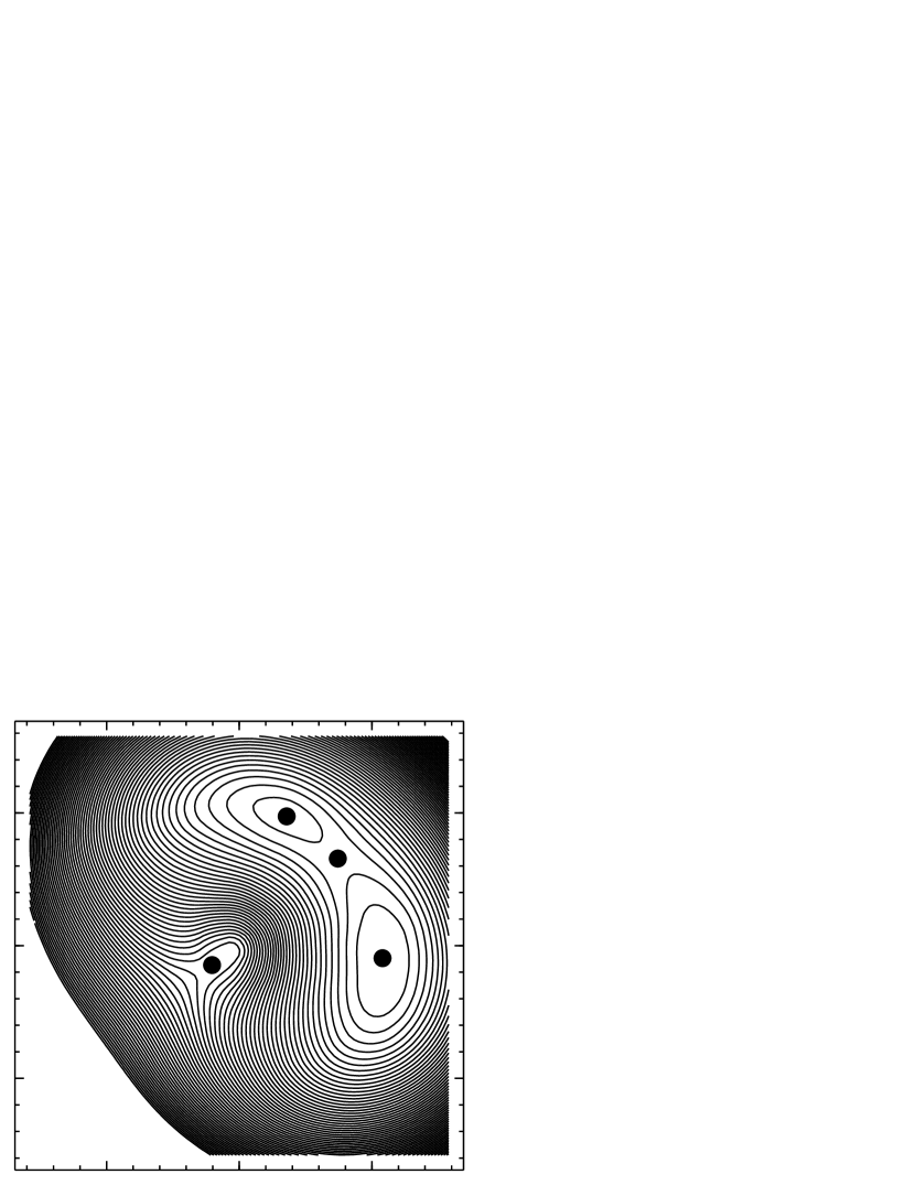
Figure 7: Models for B1422+231. Top panel: ensemble-average mass map, a miniature of which appears in Fig. 3. Second panel: mass map of a randomly chosen sample model from the ensemble; note the larger pixel-to-pixel variation. Third panel: lens potential for the galaxy in the sample model (external shear potential omitted); we see here how solving for the potential automatically smoothes out small-scale fluctuations in the mass. Bottom panel: arrival-time surface for the sample model; note that no spurious extra images are present.

Could this result be an artifact of the pixelated method? We must consider the possibility that the ensembles contain models with irregular structures not present in real galaxies, because irregular structures would tend to get washed out in ensemble averages while still contributing a large scatter to $\Delta\varphi$. We can spot-check for this possibility by inspecting individual models from the ensembles. In Figs. 7 and 8 we do so for B1422+231 and J1411+521 respectively. B1422+231 is an axial quad, as we have already noted, and has $\Delta\varphi/\varphi\simeq 4\%$, while J1411+521 is a core quad with $\Delta\varphi/\varphi\simeq 20\%$. For each of these lenses, we arbitrarily select model no. 100 out of the ensemble of 200, and show its mass profile, lens potential, and arrival-time surface. Comparing the two mass maps with the corresponding ensemble-average mass maps shown in miniature in Figs. 3 and 4, it is clear that ensemble averages smooth out pixel-to-pixel variation. But such variation affects only the second derivative of the lens potential; the potential itself is always smooth, as these figures show. Furthermore, the arrival-time contours show no spurious extra images. When we examine many more individual models spurious images do sometimes appear, but rarely (perhaps 10% of models). The remaining noticeable difference between the sample and ensemble-average maps is varying ellipticity, especially the twisting ellipticity in Fig. 8 for J1411+521. Roughly speaking, the sample model for J1411+521 suggests a bar but the ensemble as a whole does not.

We can further test whether our models are exaggerating the scatter in time delays by comparing with Table 2 in Kochanek (2002). The table shows that (a) for the axial doubles 1520+530, 1600+434, 2149-274, the approximation $H_{0}\simeq A(1-\langle\kappa\rangle)+B\langle\kappa\rangle\alpha+C$ comes to within $\sim 5\%$ of a full model, and is a slight improvement on the lowest order approximation $H_{0}\simeq A(1-\langle\kappa\rangle)$, while (b) for the inclined quad B1115+080, the simpler approximation comes within about $15\%$ of a full model, and introducing $B,C$ makes the approximation worse. The $\Delta\varphi/\varphi$ that we compute are very consistent with these levels. In other words, for these lenses pixelated models give a similar estimate for the size of the error term in Eq. (4) as do Kochanek’s original parameterized models.

We thus conclude that the identification by Kochanek of $\langle\kappa\rangle$ as a tracker of the steepness degeneracy was an important insight, but the attempt to improve beyond $H_{0}\simeq(1-\langle\kappa\rangle)$ had limited success because correction term(s) due to shape degeneracies are not a function of $\langle\kappa\rangle$. Consequently, the error term in Eq. (4) is not in practice a negligible effect: on the one hand $\Delta R/R$ is not $\ll 1$ except in core quads; on the other hand, in core quads $\varphi$ is itself small, and hence small changes in the mass profile can produce large fractional changes in $\varphi$. Furthermore, the possibility of shape degeneracies of order $\Delta R/R$ (i.e., lower order than the error term) is not ruled out.

Returning to Figs. 3–6 and examining them in more detail, we see that both $\varphi$ and its dispersion depend on the morphology, but in different ways. The time delay increases with morphology as follows:

1. core quads ($\varphi\leq 1.5$),

2. inclined quads ($1.5\leq\varphi\leq 2$),

3. axial quads ($2\leq\varphi\leq 4$),

4. doubles ($3\leq\varphi\leq 8$).

The relation of $\varphi$ to the morphology of the image distribution in the lens is discussed in Saha (2004).

The total dispersion in $\varphi$ without constraining $\langle\kappa\rangle$ is of order 25% for all morphologies, though we have only shown B1422+231 here. But if $\langle\kappa\rangle$ is constrained, thus pegging the steepness degeneracy, the residual variation in time delays increases not like $\varphi$, but as follows:

1. axial systems, whether doubles or quads have $\Delta\varphi/\varphi\sim$ 5–15%,

2. inclined systems have $\Delta\varphi/\varphi\sim$ 5–20%,

3. core quads $\Delta\varphi/\varphi\sim$ 5–20%,

4. and strongly asymmetric lenses have $\Delta\varphi/\varphi\sim$ of 25% or more.

$\Delta\varphi/\varphi$ tracks the relative contribution of shape degeneracies. Perhaps not surprisingly, shape degeneracies are most important in asymmetric lenses.

3 Discussion

The steepness degeneracy in lensing is now well understood. The above numerical experiments attempt to estimate the effect of other degeneracies. This is done by searching through mass models at fixed image-positions, time-delay ratios (where applicable), and mean annular density $\langle\kappa\rangle$. The additional degeneracies, quantified approximately by $\Delta\varphi/\varphi$ at fixed $\langle\kappa\rangle$, turn out for some lenses to be as important as steepness.

What then are the additional important degeneracies beyond steepness? Do common parametric forms for lenses already allow for the other degeneracies, and if not, what new parameters are needed? Detailed answers to these questions require more research, but we can deduce partial answers by thinking about the arrival-time surface. In the Introduction we classified degeneracies into steepness and shape, with the stipulation that the latter category can be further subdivided depending on how many image observables we care to consider. In this Section we go a little further and attempt a more quantitative, but still intuitive classification.

Recall that the steepness degeneracy amounts to a homogeneous stretching or shrinking of the time scale in the arrival-time surface. Imagine now that we stretch the time scale on the E side and shrink it on the W side, preserving the image positions. No change is required in the circularly averaged $\langle\kappa\rangle$. The resulting models are not steepness-degenerate, but the time delay between E and W images will change, producing a shape-degeneracy transformation. This particular kind is allowed only in asymmetric lenses, but there it may well be as important as the steepness degeneracy. Next, let us imagine stretching the time scale on the E and W quadrants while shrinking it on the N and S quadrants. Such a transformation, allowed in inversion symmetric lenses, is likely to most affect core quads, and inclined quads and doubles to a lesser extent, but not axial systems. Further, we can imagine a transformation that shrinks the time scale at small radii and stretches it at large radii.

We can thus imagine a hierarchy of lensing degeneracies, from an $m=0$ mode (the steepness degeneracy) through $m=1,2,$ etc. representing various shape degeneracies. This is reminiscent of basis functions in cylindrical coordinates, but we emphasize that shape degeneracies are not additive modes in the arrival-time surface, still less so in the mass profile — they are multiplicative modes in the arrival-time surface, and in the mass profile their form will be more complicated.

The steepness degeneracy is special in that it rescales the arrival time surface homogeneously, leaving time-delay ratios and magnification ratios unaffected, while there is no guarantee that shape degeneracies will preserve time-delay and magnification ratios. The image elongation information by itself, as measured in weak lensing does not break shape degeneracies, but having having many weakly lensed images would help to constrain the shape of the arrival time surface. Sources at multiple redshifts will break steepness, and help reduce shape degeneracy.

We can try and guess the sort of mass-profile feature that will produce an $m=2$ mode. By analogy with the steepness degeneracy, suppose an elliptical mass profile is steeper along the long axis than the short axis; this corresponds to ellipticity decreasing with increasing radius, and it seems plausible that it will increase time delays along the long-axis direction and decrease delays along the short-axis direction. In general we suggest that ellipticity varying or twisting with radius as the signature of $m=2$ and higher modes. Re-examining our early models of the inclined quad B1115+080 (Saha & Williams, 1997) the role of such features in fitting time delays is already apparent; at the time we commented briefly on it but had no interpretation.

The above suggests interpreting the degeneracy given by Zhao & Qin (2003) as a mixture of steepness and shape degeneracies. Their Fig. 2 illustrates the transformation of an arrival-time surface, which appears to be an $m=2$ stretching/shrinking followed by an $m=0$ stretching with the effects canceling at the image positions but not globally. (Note that the left- and right-hand sides of their arrival-time plot actually correspond to a $90^{\circ}$ change of position angle, not $180^{\circ}$.)

In the Zhao-Qin example, the ellipticity in the potential comes entirely from external shear and the main lens is circular. But in our Figs. 3–6, varying and twisting ellipticity is a common feature, especially in inclined systems. The axial systems in these figures tend not to show twisting ellipticity. Recall also from our numerical results that axial systems like B1422+231 tend to have the lowest $\Delta\varphi/\varphi$, that is to say, steepness dominates. Individual models of axial systems may still contain twisting ellipticity; however, clockwise and anti-clockwise twists are equivalent if the image morphology is axial, hence such twists will tend to cancel in the ensemble average. For inclined image morphologies, clockwise and anti-clockwise twists in the density are not equivalent, and will tend to survive in an ensemble average. We may ask whether the pixelated method tends to exaggerate twisting ellipticity. The blind tests in Williams & Saha (2000) are reassuring in this regard; no spurious twisting appears in the ensemble-average models.

We remark that in galaxy dynamics, twisting ellipticity arises naturally in at least two ways: differential rotation leading to spiral features, and projection of triaxial features. Because these and other shape features can be important in real lenses, the errors in derived $H_{0}$ must incorporate all of the degeneracies(Saha et al., 2006).

The arguments in this Discussion are hand-waving, but they indicate that the issue of varying/twisting ellipticity needs closer attention. One project that is now called-for is to map the degeneracies in pixelated models in detail, using principal components analysis or similar on model ensembles, to see if a hierarchy of degeneracies indeed emerges. Another project is to incorporate ellipticities that can vary or twist with radius into parametric models.

Figure 1: Plot of $\langle\kappa\rangle$ against $\varphi$ for an ensemble of 200 models of B1422+231, using the observed image positions and some plausible time delays.

Figure 2: Plot of $\alpha$ against $\varphi$ for 200 models of B1422+231, with $\langle\kappa\rangle$ fixed at the ensemble average from Fig. 1.

Figure 3: Plot of the dispersion $\Delta\varphi/\varphi$ against median $\varphi$ at fixed $\langle\kappa\rangle$. Each plotting symbol is the ensemble-average mass map of the lens, with the image-positions indicated. The mass contours are in logarithmic steps of $10^{0.4}$ (like a magnitude scale) and the third contour from the outside is always $\kappa=1$. But note that the spatial scale is different for different lenses. Lens names on the upper right form a key. All models except J0414+053 have inversion symmetry.

Figure 4: Continuation of Figure 3. All models have inversion symmetry.

Figure 5: Continuation of Figures 3 and 4. In the case of the ten-image system B1933+503, we used all images for modeling, but considered $\varphi$ for the core quad, as indicated. All models have inversion symmetry.

Figure 6: Similar to Figs. 3–5, but using a different scale. All the lenses are asymmetric with very large $\Delta\varphi/\varphi$.

Figure 8: Like Fig. 7 but for J1411+521. The top panel appears in miniature in Fig. 4. The sample model (middle panel) has a bar, while the ensemble as a whole does not.

References

- Bartelmann & Narayan (1995) Bartelmann. M. & Narayan, R, 1995, Proceedings, Dark Matter, Univ. of Maryland, College Park, Maryland, October, 1994. New York: American Institute of Physics (AIP). Eds: S.S. Holt & C.L. Bennett. AIP Conference Proceedings, Vol. 336, 1995, p.307
- e.g., Bender et al. (2005) Bender, R. et al. 2005, ApJ, 631, 1
- Bradac et al. (2004) Bradač, M., Lombardi, M. & Schneider, P. 2004, Å, 424, 13
- Capellari et al. (2006) Capellari, M. 2006, MNRAS, 366, 1126
- Falco et al. (1985) Falco, E. E., Gorenstein, M. V. & Shapiro, I. I. 1985, ApJ, 289, L1
- Gorenstein et al. (1988) Gorenstein, M. V., Shapiro, I. I. & Falco, E. E. 1988, ApJ, 327, 693
- Jakobsson et al. (2005) Jakobsson, P., Hjorth, J., Burud, I., Letawe, G., Lidman, C. & Courbin, F. 2005, A&A, 431, 103
-
Kochanek et al. (1998)
Kochanek, C.S., Falco, E.E., Impey, C., Lehár, J., McLeod, B., Rix,
H.-W. 1998,
cfa-www.harvard.edu/glensdata - Kochanek (2002) Kochanek, C.S. 2002, ApJ, 578, 25
- Kochanek et al. (2006) Kochanek, C.S, Morgan, N.D, Falco, E.E., McLeod, B.A., Winn, J.N., Dembicky, J., & Ketzeback, B. 2006, ApJ, 640, 47
- Morgan et al. (2006) Morgan, N.D., Kochanek, C.S., Falco, E.E., & Dai, X. 2006, astro-ph/0605321
- Oguri & Kawano (2002) Oguri, M. & Kawano, Y. 2002, MNRAS, 338, L25
- Paczyński (1986) Paczyński, B. 1986, ApJ, 301, 503
- Raychaudhury et al. (2003) Raychaudhury, S., Saha, P. & Williams, L.L.R. 2003, AJ, 126, 29
- Saha (2000) Saha, P. 2000, AJ, 120, 1654
- Saha (2004) Saha, P. 2004, A&A, 414, 425
- Saha et al. (2006) Saha, P., Coles, J., Macciò, A.V., & Williams, L.L.R. 2006, ApJ, in press, astro-ph/0607240
- Saha & Williams (1997) Saha, P., & Williams, L.L.R. 1997, MNRAS, 292, 148
- Saha & Williams (2003) Saha, P., & Williams, L.L.R. 2003, AJ, 125, 2769
- Saha & Williams (2004) Saha, P., & Williams, L.L.R. 2004, AJ, 127, 2604
- Schneider & Seitz (1995) Schneider, P. & Seitz, C. 1995, A&A, 294, 411
- e.g., Schechter (2004) Schechter, P.L. 2004, Proceedings of IAU Symposium No. 225, The Impact of Gravitational Lensing on Cosmology, eds: Y. Mellier & G. Meylan
- Treu & Koopmans (2004) Treu, T. & Koopmans, L.V.E. 2004, ApJ, 611, 739
- Trotter et al. (2000) Trotter, C.S., Winn, J.N. & Hewitt, J.N. 2000, ApJ, 535, 671
- Vuissoz et al. (2006) Vuissoz, C., et al., 2006, astro-ph/0606317
- Wambsganss & Paczyński (1994) Wambsganss, J. & Paczyński, B. 1994, AJ, 108, 1156
- Williams & Saha (2000) Williams, L.L.R. & Saha, P. 2000, AJ, 119, 439
- Wucknitz (2002) Wucknitz, O. 2002, MNRAS, 332, 951
- Zhao & Qin (2003) Zhao, H.-S. & Qin, B. 2003, ApJ, 582, 2