The survival and disruption of CDM micro-haloes: implications for direct and indirect detection experiments

Abstract

If the dark matter particle is a neutralino then the first structures to form are cuspy cold dark matter (CDM) haloes collapsing after redshifts $z\approx 100$ in the mass range $10^{-6}-10^{-3}\,{\rm M_{\odot}}$. We carry out a detailed study of the survival of these micro-haloes in the Galaxy as they experience tidal encounters with stars, molecular clouds, and other dark matter substructures. We test the validity of analytic impulsive heating calculations using high resolution $N$-body simulations. A major limitation of analytic estimates is that mean energy inputs are compared to mean binding energies, instead of the actual mass lost from the system. This energy criterion leads to an overestimate of the stripped mass and underestimate of the disruption timescale since CDM haloes are strongly bound in their inner parts. We show that a significant fraction of material from CDM micro-haloes can be unbound by encounters with Galactic substructure and stars, however the cuspy central regions remain relatively intact. Furthermore, the micro-haloes near the solar radius are those which collapse significantly earlier than average and will suffer very little mass loss. Thus we expect a fraction of surviving bound micro-haloes, a smooth component with narrow features in phase space, which may be uncovered by direct detection experiments, as well as numerous surviving cuspy cores with proper motions of arc-minutes per year, which can be detected indirectly via their annihilation into gamma-rays.

1 Introduction

If dark matter is composed mainly of the lightest supersymmetric partner particle, the neutralino, the first self-gravitating structures in the Universe are Earth-mass haloes forming at high redshifts (Hofmann, Schwarz & Stöcker, 2001; Diemand, Moore & Stadel, 2005). As many as $10^{15}$ could be within our Galactic halo today. These abundant cold dark matter (CDM) micro-haloes have cuspy density profiles that can withstand the Galactic tidal field at the solar radius. The numbers of such haloes that lie within the vicinity of the solar system depends on how many survive the complex merging history of early hierarchical structure formation. $N$-body simulations of CDM satellites indicate that tightly bound cusps are very stable against tidal stripping (Kazantzidis et al. 2004), and therefore dense micro-haloes accreting late onto more massive structures may survive relatively intact. The exact distribution of dark matter in the solar vicinity is important for direct and indirect dark matter detection experiments.

Substructures that survive the merging process will experience continuous perturbative encounters with stars, molecular clouds, and other dark matter subhaloes. As discussed in Diemand, Moore & Stadel (2005), we expect that these encounters lead to some mass loss but that the cusps of most micro-haloes remain intact. Recent studies by Zhao et al. (2005a, b), Green & Goodwin (2006) and Berezinsky, Dokuchaev & Eroshenko (2006) have raised the question whether these first haloes would be completely disrupted by close encounters with stars. Crossing the Galactic disc would also cause additional tidal heating. Moore et al. (2005) argued that the analytical impulse approximation and the semi-analytic models used in these studies may not fully describe the disruption of the high-density inner cores. Particle orbits deep in the cusp may remain adiabatically invariant to the perturbations and preserve the structure of the cusp. Only direct numerical simulations can describe these complex dynamical processes. In this paper, we use several sets of high resolution $N$-body simulations to test the validity of analytical heating models.

An important factor in the survival statistics of micro-haloes is how many survive similar-mass mergers during the build-up of the Galactic halo (Diemand, Kuhlen & Madau, 2006). Even if only a few percent survive the hierarchical growth, many micro-haloes would still lie within one parsec from the Sun. Their dense cuspy cores would be sources of gamma-ray emission due to self-annihilation, which could be uniquely distinguished by their high proper motions on the sky of the order arc-minutes per year (Moore et al. 2005, Koushiappas 2006).

2 Heating by stars in the solar neighbourhood

There are various ways to define a virialized halo. The approach often used in cosmological simulations, which we adopt here, is that dark haloes virialize when their average density equals $\Delta=200$ times the mean density of the Universe, $\bar{\rho}(z)=3\Omega_{0}H_{0}^{2}(1+z)^{3}/8\pi G$. Here $H_{0}$ is the Hubble constant, $\Omega_{0}$ is the matter density parameter, and $z$ is the redshift of virialization. Then the virial radius of the halo, defined by the relation $M_{\rm vir}\equiv{4\pi\over 3}R_{\rm vir}^{3}\Delta\bar{\rho}(z)$, is

$$R_{\rm vir}=0.31\,(1+z)^{-1}\left({M_{\rm vir}\over 10^{-6}\,{\rm M_{\odot}}}\right)^{1/3}\mbox{pc},$$ (1)

for $\Omega_{0}=0.3$ and $H_{0}=70\,\mbox{km s}^{-1}\,\mbox{Mpc}^{-1}$. The virial velocity is defined by the relation $V_{\rm vir}^{2}\equiv GM_{\rm vir}/R_{\rm vir}$:

$$V_{\rm vir}=12\,(1+z)^{1/2}\left({M_{\rm vir}\over 10^{-6}\,{\rm M_{\odot}}}\right)^{1/3}\mbox{cm s}^{-1}.$$ (2)

These parameters determine the binding energy of the haloes, which can be expressed using the half-mass radius of the system: $E_{\rm b}\approx 0.2GM_{\rm vir}/R_{\rm 1/2}$ (Spitzer, 1987). Density profiles of dark matter haloes in cosmological simulations are often described by the NFW model with a concentration parameter, $c$. For $c<10$, the radius containing half of the virial mass is approximately $R_{1/2}\approx(5c)^{-1/4}\,R_{\rm vir}$. High-redshift haloes have typically low concentrations, such that $R_{1/2}\approx 0.5R_{\rm vir}$. Therefore, the binding energy of first haloes is $E_{\rm b}\approx 0.4V_{\rm vir}^{2}$.

As these small haloes merge into larger systems, two effects may modify their structure: tidal truncation by the host galaxy and tidal heating by massive, fast-moving perturbers (stars, molecular clouds, other dark matter substructures).

In the vicinity of the Sun, the matter density is dominated by stars, which we assume to have the same mass $m_{*}=0.7\,{\rm M_{\odot}}$. The stellar mass density is $m_{*}n_{*}\approx 0.1\,{\rm M_{\odot}}$ pc^-3 (Binney & Merrifield, 1998), which is a half of the total density of the disc calculated from the Oort limit (Bahcall, 1984). In order to remain gravitationally self-bound, the micro-haloes must have an average density above roughly $2m_{*}n_{*}$.

Fast encounters with massive perturbers increase the velocity dispersion of dark matter particles and reduce a halo’s binding energy. A distant encounter at an impact parameter $b$ with a relative velocity $V_{\rm rel}$ increases the energy per unit mass on the average by

$$\Delta E_{1}(b)\approx{1\over 2}\left({2Gm_{*}\over b^{2}\,V_{\rm rel}}\right)^{2}{2\over 3}\left<r^{2}\right>,$$ (3)

where $\left<r^{2}\right>\sim R_{1/2}^{2}$ is the ensemble average of the particle distance squared from the centre of the micro-halo.

At very small impact parameters, $b<b_{1}$, a single encounter would be sufficiently strong to unbind the whole halo: $\Delta E_{1}(b_{1})=E_{\rm b}$. As we show later in section 4, a small central part always survives even such a strong perturbation, apart from direct collisions with $b=0$. Nevertheless, it is instructive to define the disruptive encounter threshold, which is given by

$$b_{1}=a_{\rm c}\left({Gm_{*}R_{\rm vir}\over V_{\rm rel}V_{\rm vir}}\right)^{1/2}\approx 0.2\,(1+z)^{-3/4}\ {\rm pc},$$ (4)

where $a_{\rm c}\approx 0.96\,(c/3)^{-1/8}$. Equation (3) is strictly valid only in the tidal approximation, $b\gg R_{\rm vir}$. An encounter at $b_{1}$ falls in that regime for redshifts $z<50$, which is appropriate for our consideration of the micro-haloes.

The number of encounters over time $t$ as a function of impact parameter is $dN_{\rm enc}(b)=n_{*}V_{\rm rel}t\,2\pi bdb$, where $n_{*}$ is the number density of stars. We can obtain the cumulative effect of multiple non-disruptive encounters by integrating over the impact parameter:

$$\Delta E_{\rm tid} = \int_{b_{1}}^{b_{\rm max}}\Delta E_{1}(b)\,{dN_{\rm enc}\over db}\,db$$ (5)

$$= 0.4a_{\rm c}^{4}\pi{G^{2}m_{*}^{2}R_{\rm vir}^{2}n_{*}t\over V_{\rm rel}}\left({1\over b_{1}^{2}}-{1\over b_{\rm max}^{2}}\right).$$

The upper limit of integration is set by the condition that the encounter is impulsive, i.e. the duration of the encounter $b/V_{\rm rel}$ is shorter than the orbital time of particles in the halo, $R_{\rm vir}/V_{\rm vir}$. The maximum impact parameter is given by

$$\left({b_{\rm max}\over b_{1}}\right)^{2}\approx a_{\rm c}^{2}{V_{\rm rel}^{3}\,R_{\rm vir}\over Gm_{*}V_{\rm vir}}\gg 1.$$ (6)

The ratio of the tidal heating energy in non-disruptive encounters to the binding energy is

$${\Delta E_{\rm tid}\over E_{\rm b}}=a_{\rm c}^{2}\pi{Gm_{*}n_{*}tR_{\rm vir}\over V_{\rm vir}}.$$ (7)

We can also calculate the effect of disruptive encounters, with $b<b_{1}$. The number of such encounters is simply

$$N_{\rm enc}(<b_{1})=\pi b_{1}^{2}n_{*}V_{\rm rel}t=a_{\rm c}^{2}\pi{Gm_{*}n_{*}tR_{\rm vir}\over V_{\rm vir}}.$$ (8)

This number is the same as equation (7) meaning that the cumulative effect of disruptive encounters is the same as that of non-disruptive encounters. The total disruption probability, $N_{\rm tot}$, is then twice that given by equation (7).

To calculate this disruption probability, we note that while stars in the solar neighbourhood move on approximately circular orbits around the Galactic centre, small dark matter haloes would be moving on isotropic orbits inclined with respect to the Galactic disc. Their expected vertical velocity is $V_{z}\approx 200$ km s^-1. The crossing time of the disc with a scale height of $H=0.2$ kpc is $2H/V_{z}=2\times 10^{6}$ yr. In the solar neighbourhood, haloes would cross the disc every $10^{8}$ yr and have about 100 crossings in the Hubble time. The total amount of time the haloes would spend in the region of high stellar density $m_{*}n_{*}$ is then $t_{d}\sim 2\times 10^{8}$ yr. The total disruption probability is

$$N_{\rm tot} = 2\,N_{\rm enc}(<b_{1})$$ (9)

$$= \left({1+z\over 131}\right)^{-3/2}\left({m_{*}n_{*}\over 0.1\,{\rm M_{\odot}}\,{\rm pc}^{-3}}\right)\left({t_{d}\over 2\times 10^{8}\,{\rm yr}}\right).$$

Therefore, the haloes virialized after redshift $z=130$ should suffer significant mass loss by passing stars in the solar neighbourhood. Due to biased halo formation typical subhaloes in the solar neighbourhood come form $2\sigma$ fluctuations (Diemand, Madau & Moore 2005), i.e. they virialize at half the expansion factor (or twice the (z + 1) value) than typical haloes of the same mass in the field (i.e. $1\sigma$ peaks). A formation time of z = 130 corresponds to about a $3\sigma$ peak. Such early structure formation is not uncommon in dense environments, for example the small, over dense region simulated in Diemand, Kuhlen & Madau (2006) already contains 845 micro-haloes at z = 130. A fraction of about 20% of the local mass comes from peaks above $3\sigma$ (Diemand, Madau & Moore 2005), implying that approximately 20% of the local subhalo population should therefore not suffer significant mass loss.

3 Heating by dark matter substructure

Virialized, self-gravitating subhaloes within larger haloes (the substructure) will also kinematically heat and disrupt their small cousins [c.f. Boily et al. (2004)]. $N$-body simulations (Diemand, Moore & Stadel, 2004) show that the number of subhaloes with masses above $M$ within a host of mass $M_{\rm host}$ scales as

$$N_{\rm sub}(>M/M_{\rm host})\approx\left({M\over 10^{-2}\,M_{\rm host}}\right)^{-1}.$$ (10)

Since stars occupy only a small fraction of the volume of their host haloes, it is important to consider if the tidal heating by dark matter subhaloes can disrupt a significant fraction of micro-haloes.

The analysis of section 2 can be generalised for perturbers with a range of masses, $M_{\rm vir}<M<10^{-2}\,M_{\rm host}$. Let $f\equiv M/M_{\rm host}$ be the dimensionless subhalo mass. The threshold impact parameter, at which a single encounter with subhalo $f$ is disruptive, is $b_{1}^{2}(f)\approx fV_{\rm host}R_{\rm host}R_{\rm vir}/V_{\rm vir}$, where we assumed the relative velocity to be the virial velocity of the host halo, $V_{\rm rel}\approx V_{\rm host}$. However, for most subhaloes this impact parameter is smaller than their size, $R_{\rm sub}\approx r[M_{\rm sub}/3M_{\rm host}(r)]^{1/3}$, which is determined by tidal truncation at distance $r$ from the centre of the host halo. Tidal approximation applies only at $b>b_{\rm min}=R_{\rm sub}$. Therefore, most encounters will be non-disruptive.

The cumulative heating by multiple non-disruptive encounters with subhaloes of mass $M_{\rm sub}=fM_{\rm host}$ is [see equation (5)]:

$${\Delta E_{\rm tid}(f)\over E_{\rm b}}={\pi G^{2}M_{\rm sub}^{2}R_{\rm vir}^{2}t\over V_{\rm host}V_{\rm vir}^{2}b_{\rm min}^{2}}{dn_{\rm sub}\over df},$$ (11)

where $dn_{\rm sub}\over df$ is the number density of subhaloes $f$. Taking an NFW model for the smooth component of the Galactic halo and restricting our analysis to the inner part of the halo, $r\la r_{s}\approx 20$ kpc, we find the subhalo’s truncation radius $R_{\rm sub}\approx r_{s}(fr/r_{s})^{1/3}$. The density of subhaloes, assuming they have not been completely disrupted, is

$${dn_{\rm sub}\over df}\approx{10^{-2}f^{-2}\over 4\pi g(c)r_{\rm s}^{2}r},$$ (12)

where $g(c)\equiv\ln{(1+c)}-c/(1+c)\approx 1.6$ for a concentration parameter $c=12$ (Klypin, Zhao & Somerville, 2002). For the Galaxy, a Hubble time corresponds to $t\sim 5R_{\rm host}/V_{\rm host}$.

Thus for the inner halo,

$${\Delta E_{\rm tid}(f)\over E_{\rm b}} = {5\times 10^{-2}c^{5}\over 4g(c)}\left({tV_{\rm host}\over 5R_{\rm host}}\right){R_{\rm vir}^{2}V_{\rm host}^{2}\over R_{\rm host}^{2}V_{\rm vir}^{2}}$$ (13)

$$\times f^{-2/3}\left({r\over r_{\rm s}}\right)^{-5/3}.$$

Integrating over all subhaloes, $f<0.01$, we find

$${\Delta E_{\rm tid}\over E_{\rm b}}\approx 0.063\left({r\over r_{\rm s}}\right)^{-5/3}.$$ (14)

Thus, mini-haloes may be disrupted by repeated encounters with more massive haloes within $r\la 0.2r_{\rm s}\approx 4$ kpc from the centre of the Galaxy.

4 Numerical tests of the impulsive approximation

In this section we test the response of a CDM micro-halo to repeated impulsive encounters using N-body calculations in order to test the validity of the impulse approximation, and to study in detail how the internal structure of the micro-haloes evolve with time.

The initial state for the micro-halo is an equilibrium profile with the same structural parameters as found by Diemand, Moore & Stadel (2005) at $z=26$, the epoch at which such structures are typically accreted into larger mass systems. This halo obeys a cuspy density profile, the general $\alpha,\beta,\gamma$ law (Hernquist, 1990):

$$\rho(r)=\frac{\rho_{0}}{\left({\frac{r}{r_{\rm s}}}\right)^{\gamma}\left[{1+\left({\frac{r}{r_{\rm s}}}\right)^{\alpha}}\right]^{\frac{\beta-\gamma}{\alpha}}}\qquad(r\leq R_{\rm micro}),$$ (15)

with $\alpha=1.0$, $\beta=3.0$ and $\gamma=1.2$. The mass of the halo is $M_{\rm micro}=10^{-6}\,{\rm M_{\odot}}$ within the z = 26 virial radius $R_{\rm micro}=0.01$ pc. The concentration parameter is low, $R_{\rm micro}/r_{\rm s}=1.6$, typical of micro-haloes in the field at z = 26. Some experiments we repeated with micro-haloes having concentrations of 3.2. The typical local subhalo forms earlier (by about a factor of two in redshift, see Diemand, Madau & Moore 2005) than the average micro-halo in the field. Therefore the typical local subhalo might be twice as concentrated and more robust against mass loss. However, to be conservative we use the low concentration of 1.6 throughout this paper unless stated otherwise. For numerical stability of the profile, we make a realization of this halo extending to approximately $4\,R_{\rm micro}$ using the techniques of Kazantzidis, Magorrian & Moore (2004). At $r>R_{\rm micro}$, the density profile falls off exponentially as $\exp(-r/r_{\rm decay})$, with $r_{\rm decay}=0.3\,R_{\rm micro}$. The total mass of the system is therefore $1.81\,M_{\rm micro}$. We use $10^{6}$ particles of equal mass, $m_{\rm p}=1.81\times 10^{-12}{\rm M_{\odot}}$. The force calculations have a softening length of $0.005\,R_{\rm micro}$.

We then subject the equilibrium micro-halo to a series of impulsive encounters with a star of mass $m_{*}=0.7\,{\rm M_{\odot}}$, the mean mass per star in the disc of the Galaxy. First we run six simulations, which differ in the minimal distance from the star to the centre of the micro-halo. For these six simulations the impact parameters are $b=0.005,0.01,0.02,0.05,0.1,1$ pc. In all runs the star moves with the relative velocity $V_{\rm rel}=300$ km s^-1. The initial separation of the star and the halo along the direction of motion is three times the impact parameter or three times the micro-halo radius of the halo, whichever is the greater. After the star reaches the point of closest approach, we let it move away the same distance from the halo. Then we remove the star and let the system evolve in isolation for $3\times 10^{8}$ yr, which corresponds to 20 crossing times of the halo. Similar experiments date back to e. g. Aguilar & White (1985).

Each encounter increases the internal energy of the micro-halo. Following the perturbation, the system undergoes a series of virial oscillations (contraction and expansion) until the potential relaxes into a new equilibrium configuration (Gnedin & Ostriker, 1999). Depending on the strength of the perturbation, this potential relaxation takes between 10 and 20 crossing times of the halo. The final configuration has a lower binding energy and some particles may escape the system entirely.

Fig. 1 shows the energy change per particle for a flyby at $b=0.02$ pc at two different times: directly following the encounter and after the potential relaxation. The duration of the encounter, $\tau=2b/V_{\rm vel}\approx 130$ yr, is much shorter than the dynamical (crossing) time of the particles in the micro-halo, $t_{\rm dyn}\approx 1.5\times 10^{7}$ yr. Therefore, we expect that the tidal heating can be calculated in the impulsive approximation [c.f. equation (3)]. For ensemble-average of stars with initial energy $E$, the energy per unit mass increases by the amount

$$\left<\Delta E\right>={4\over 3}\left({Gm_{*}\over b^{2}\,V_{\rm rel}}\right)^{2}r^{2}.$$ (16)

This prediction is plotted next to the numerical result (squares) in Fig. 1 and agrees with it very well.

Subsequent potential relaxation reduces the depth of the potential well of the system, leading to another effective energy change. Gnedin & Ostriker (1999) found that this additional energy change can be approximated as a constant fraction of the initial potential, $\Phi_{\rm i}$:

$$\Delta E_{\rm pot}(r)=c\,(-\Phi_{\rm i}(r)),$$ (17)

where the constant $c$ is such that the sum of $\Delta E_{\rm pot}(r)$ over all particles is twice the initial energy change of the system, $\Delta E_{1}(b)$, as required by the virial theorem. The final energy difference is $\left<\Delta E\right>+\Delta E_{\rm pot}$. This prediction is plotted next to the numerical result (triangles) in Fig. 1

Figure 1: Energy change per particle as a function of radius immediately following the perturbation (squares) and after potential relaxation (triangles), for the encounter with $b=0.02$ pc.

and again provides a very good fit.

Fig. 2

Figure 2: Energy change per particle as a function of radius immediately following the perturbation, for encounters with different impact parameters $b$.

shows the energy changes immediately following the encounters at different impact parameters, $b$. The analytical formula (16) provides a good description of the numerical results, except in cases of extremely strong perturbations when the energy changes by more than 100%, $\left<\Delta E\right>>|E|$.

Fig. 3

Figure 3: Energy change per particle as a function of radius after potential relaxation, for encounters with different impact parameters $b$.

shows the final energy redistribution after potential relaxation, for encounters with different impact parameters, $b$. Equations (16) and (17) describe the effect very accurately.

The change of the micro-halo potential leads to the change of the density profile. Particles that gain enough energy escape the system form unbound tidal tails. The final density profiles for the encounters with different impact parameters are shown in Fig. 4.

Figure 4: Density profile of the micro-halo in a new equilibrium, after encounters with different impact parameters, $b$. The arrow indicates the micro-halo radius.

The amount of mass stripped from the halo depends on the definition of the bound mass. The density of the outer halo profile extends as $r^{-3}$ beyond the nominal micro-halo radius, and all of the particles are initially bound. We use two practical definitions. (i) We have defined an effective maximum radius, $R_{\rm max}\equiv 4R_{\rm micro}$, beyond which all particles are assumed to be lost of the micro-halo. In practice, this radius can be set by the external tidal field. (ii) We have also defined an effective tidal potential at that radius, $\Phi_{\rm t}\equiv\Phi(R_{\rm max})$. We use this tidal potential to construct another definition of unbound particles, as those with $E>\Phi_{\rm t}$. After the potential relaxation, the new potential $\Phi$ is used to define $\Phi_{\rm t}$ at the same fixed radius $R_{\rm max}$.

Fig. 5

Figure 5: Total energy change of all particles immediately following the perturbation, as a function of impact parameter (filled squares) and the analytical prediction in the impulse approximation (solid line).

shows the change of the total energy of the system immediately following the encounter, for all particles within $R_{\rm max}$. It is well described by equation (3), which is plotted as a solid line. Since the density profile of the system continues beyond the nominal micro-halo radius, the average radius for all particles is $\left<r^{2}\right>=1.63\,R_{\rm micro}^{2}$. We used this value for the plotted prediction.

Fig. 6

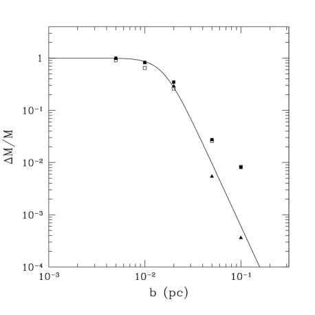
Figure 6: Mass loss of the halo as a function of the impact parameter $b$, determined using either the energy criterion, $E>\Phi_{\rm t}$ (open squares: immediately following the perturbation, filled squares: after the potential relaxation) or the position criterion, $r>R_{\rm max}$, after the potential relaxation (triangles).

shows the mass loss as a function of impact parameter, using the two definitions based on the position and energy criterion, respectively. For large impact parameters (weak perturbations), the position criterion indicates systematically lower mass loss than the energy criterion. Therefore, some particles within $R_{\rm max}$ may be unbound at the end of the simulation. In the strong perturbation regime, both criteria give similar results.

While the total energy change of the system can be computed with sufficient accuracy using the impulsive approximation, the amount of mass lost cannot. Using our numerical simulations, we seek to establish a practical relation between $\Delta M/M$ and $\Delta E/E_{\rm b}$. We find that the following equation provides a good fit to the numerical results:

$$\frac{\Delta M}{M}=\frac{1}{1+2.1\left(\Delta E\over E_{\rm b}\right)^{-1}}.$$ (18)

For weak perturbations the mass loss scales as the energy change, $\Delta M/M\approx 0.5\Delta E/E_{\rm b}$. For very strong encounters, the mass loss asymptotically approaches unity. Note however, that even for very small impact parameters, when $\Delta E/E_{\rm b}\gg 1$, a small fraction of the mass always remains bound, $\approx 2(\Delta E/E_{\rm b})^{-1}$.

A note on notation. Strictly speaking, the tidal approximation which was used to derive equation (3) is only valid for $b\gg R_{\rm micro}$. At smaller impact parameters the energy change does not scale as $b^{-4}$, but it can be calculated in the opposite asymptotic limit (e.g, Moore, 1993; Carr & Sakellariadou, 1999; Green & Goodwin, 2006). We take an alternative approach by parametrising the mass loss in our numerical simulations (equation [18]) based on the formal extrapolation of equation (3) to all values of $b$.

As Fig. 4 shows, most of the mass remaining bound to the micro-halo after strong perturbations is concentrated near its centre. It is therefore interesting to calculate the fraction of lost mass that was initially contained within the power law density cusp, at $r<r_{\rm s}$. Fig. 7

Figure 7: Mass lost inside the scale radius, $r<r_{\rm s}$, after the potential relaxation, as a function of impact parameter.

shows that this fraction scales as $\Delta M_{\rm cusp}/M_{\rm cusp}\approx(1+5(\Delta E/E_{\rm b})^{-1})^{-1}$.

We also performed another set of simulations, by repeatedly perturbing the micro-halo with the same star, with the same relative velocity and at the same impact parameter $b=0.02$ pc. After the halo has relaxed following the first encounter, we move the centre of mass of the remaining halo to the origin of the coordinate system and let a star pass by in exactly the same way and again let it relax, and then repeat the encounter a total of ten times.

The density profile of the micro-halo after $n$ encounters is shown in Fig. 8.

Figure 8: Density profile of the micro-halo after successive encounters with a star with the same mass and orbital parameters ($b=0.02$ pc), marked by the encounter number $n$.

Every encounter heats the system and strips some mass, but each successive encounter is less and less effective. Fig. 9

Figure 9: Cumulative mass loss of different micro-haloes after a number of identical encounters with $b=0.02$ pc.

shows the cumulative mass loss after each such encounter. It can be described by the following function:

$$\frac{\Delta M}{M}(n)=1-\exp\left(An^{B}\right),$$ (19)

with A = -0.34 and B = 0.87 for c = 1.6 and A = -0.23 and B = 0.81 for c = 3.2, which are also shown in Fig. 9.

We fitted each of the eleven density profiles, which are shown in Fig. 8, as well as the corresponding eleven density profiles for the halo with c = 3.2, which are not shown, with equation (15). To make the fits we used the Levenberg-Marquardt method (Marquardt, 1963) in log-log space keeping $\gamma$ fixed at 1.2. The variation of $\alpha,\beta,r_{\rm s}$ and $\rho_{0}$ from encounter to encounter is as follows: $\alpha$ increases from 1.0 to 1.5, $\beta$ increases monotonically from 3.0 to 7.0, r_s stays constant around 7.0 milli-pc for the c = 1.6 halo and around 4.0 milli-pc for the c = 3.2 halo and finally $\rho_{0}$ oscillates around 20 GeV/cm³ for c = 1.6 and decreases from 100 down to 50 GeV/cm³ in case of the other halo. The resulting profiles could now be used to calculate the net flux coming from neutralino annihilation (e.g, Koushiappas, 2006) via:

$$F=k\int^{\infty}_{r_{min}}{4\pi r^{2}\rho(r)^{2}{\rm d}r}$$ (20)

We have summed up the dependence of the flux on neutralino mass and interaction cross section in the constant $k$. The lower bound $r_{\rm min}$ is defined as the central region of the micro halo, in which the neutralinos already annihilated each other. The required number density for this to happen can be estimated with the help of

$$t_{\rm h}={1\over n\sigma v}$$ (21)

where $t_{\rm h}\approx 13$ Gyrs is the Hubble time, $\sigma v\approx 10^{-30}$ cm³s^-1 is a typical cross section and $n$ is the number density of neutralinos. For more details see Calcáneo-Roldán & Moore (1999). The minimum radius can now be computed from comparing this minimum number density with the density profile in Fig. 8. Assuming a neutralino mass of 100 GeV and deploying the above mentioned density profile, $r_{\rm min}$ comes out to be $1.6\times 10^{-14}$ pc. Fig. 10

Figure 10: The relative flux of annihilation products from different micro-haloes after a given number of encounters. The typical mass loss from a halo would lead to a decrease in flux of between a factor of two or three.

shows then the resulting annihilation flux.

In order to investigate the sensitivity of tidal heating to the structure of the micro-halo, we have run additional simulations with different initial profiles. We use the cuspy profile given by equation (15) and vary the slope $\gamma=0$, 0.5, 1, and 1.5, in addition to our fiducial value, $\gamma=1.2$. This suite of simulations is carried out using a fixed impact parameter, $b=0.02$ pc, and other parameters as in the fiducial run. Our calculations are similar to earlier studies of impulsive heating e.g. Aguilar & White (1986), who studied the structural change in systems with de Vaulouleur density profiles.

Fig. 11

Figure 11: Total mass loss from the micro-halo as a function of the inner density slope, $\gamma$, determined using the the position criterion, $r>R_{\rm max}$, after the potential relaxation (triangles), as well as the fraction of mass lost from inside the scale radius, $r<r_{\rm s}$ (squares).

shows that up to 30% more mass is lost from the cored halo ($\gamma=0$) compared to the cuspy haloes ($\gamma>1$). The effect is even stronger for the fraction of mass removed from within the scale radius, $r_{s}$: 2.5 times more material is lost from the cored halo. The strongly-bound material within the cusp is more stable against tidal disruption than that in cored profiles, which have been typically considered in previous studies of tidal heating.

In Fig. 8 we show the mass loss of the micro-halo for ten successive encounters with exactly the same impact parameter. This is unlike the situation in our Galaxy where micro-haloes orbit the disc for 10 Gyrs near the solar radius. It spends about 0.1 Gyr moving through the disc encountering stars at a relative velocity of approximately 300 km/s and a range of impact parameters. In order to model this behaviour more precisely, we use a Monte-Carlo method, which estimates the total amount of mass-loss it would suffer. We draw encounter impact parameters from a random distribution and calculate at each time the stripped mass. After each encounter, the density profile of the micro-halo changes self-consistently according to the results found earlier with the $N$-body simulations.

The mass loss due to the first encounter can easily be calculated using equation 18. From the second encounter onwards, the halo density profile changes and it is harder to strip during subsequent encounters as we have seen in Fig. 9.

The mass $M_{\rm a}$, the halo has after the $a$th encounter, determines the reduction of the mass, which is stripped in the $a+1$st encounter. This is unfortunately not a variable of equation (19). This is a function of $n$ only. So we calculate at the beginning of each encounter a “virtual encounter number” $n$, which is basically the inverse of equation (19):

$$n=\sqrt[B]{\log_{\rm e}M_{\rm a}\over A}$$ (22)

For a given $M_{\rm a}$ it computes the corresponding number of “standard encounters” with the impact parameter b = 0.02 pc from figure 9. Now we can calculate the mass $M_{\rm a+1}$ after the $a+1$st encounter. This must be a deviation from equation (18) with some weighting function $w(n,M_{\rm a})$:

$$M_{\rm a+1}=M_{\rm a}\left[1-{w(n,M_{\rm a})\over 1+2.1\left(\Delta E\over E_{\rm b}\right)^{-1}}\right],$$ (23)

This weighting function is the fraction of mass, which is stripped in the $n+1$st standard encounter divided by the fraction of mass stripped in the first standard encounter:

$$w(n,M_{\rm a})={{\Delta M\over M}(n+1)-{\Delta M\over M}(n)\over{\Delta M\over M}(1)\left(1-{\Delta M\over M}(n)\right)}$$ (24)

The ${\Delta M\over M}(n)$ can be calculated according to equation (19). This weighting function reproduces the results from Fig. 9. Keeping in mind, that $\left[1-{\Delta M\over M}(n)\right]=M_{\rm a}$, equation (23) reduces to:

$$M_{\rm a+1}=M_{\rm a}-{M_{\rm a}-\exp\left[A(n+1)^{B}\right]\over{\Delta M\over M}(1)\left[1+2.1\left(\Delta E\over E_{\rm b}\right)^{-1}\right]}$$ (25)

We use this equation recursively for each encounter and then repeat the calculation to obtain the probability distribution of final masses in Fig. 12.

Figure 12: Probability density distribution function of the final masses of different haloes

The central density (at our softening length) of a perturbed halo decreases only by a factor of about 5, whilst the total mass decreases by an average of 90 % (see Fig. 8).

5 Conclusions

We have studied the disruption of dark matter micro-haloes by stars and other substructures using both analytical impulse approximation and self-consistent $N$-body simulations. The analytic calculations presented here are quite similar to those of Green & Goodwin (2006) and we come to similar conclusions. Our calculations differed in that we used more realistic cuspy n-body models and we studied how the internal structure of these systems evolve due to perturbations. See also Angus & Zhao (2006) for an independent and complementary study. Earlier studies e.g. Aguilar & White (1986), also studied cuspy systems and found similar robustness to tidal heating in the central regions as we find. However our resolution allows us to study the response of CDM haloes deep within their central regions.

• The impulse approximation predicts that those micro-haloes in the solar vicinity which formed after z = 130 (about 80% of the local micro-halo population) should lose most of their mass due to close encounters with disc stars.

• Numerical simulations of individual encounters demonstrate that the usual condition of disruptive heating used in analytical studies, $\Delta E=E_{\rm b}$, does not lead to complete dissolution of haloes with cuspy density profiles. For the inner logarithmic slope $\gamma=1.2$, on average only 30% of the mass is lost from the system for this energy change. The relation between the fractional mass loss and the energy input in the tidal approximation is given by equation (18): $\Delta M/M\approx(1+2(\Delta E/E_{\rm b})^{-1})^{-1}$.

• The change of particle energies, after the system settles into a new virial equilibrium following the tidal encounter, is described accurately by the extension of the impulse approximation accounting for virial oscillations. An apparent resistance to tidal heating of the material deep in the cusp is due to the high binding energy inside the cusp.

• Repeated tidal encounters lead to diminishing mass loss from the same micro-halo. After 10 identical encounters at impact parameter $b=2R_{\rm vir}$, 10% of the halo still remains self-bound even though $\Delta E=5E_{\rm b}$.

Near the solar radius within the Galaxy most of the mass of the micro-haloes is tidally removed. This material forms cold streams in phase space providing a unique signal for direct detection experiments. The dense cuspy cores of these haloes survive reasonably intact, although the mass loss leads to a reduction in annihilation products of about a factor of only two to three. These cores could be distinguished by their high proper motions on the sky of the order arc-minutes per year.

References

- Aguilar & White (1985) Aguilar L. A, White S. D. M, 1985, ApJ, 295, 374
- Aguilar & White (1986) Aguilar L. A, White S. D. M, 1986, ApJ, 307, 97
- Angus & Zhao (2006) Angus G. W, Zhao H. S, 2006, astro-ph/0608580
- Bahcall (1984) Bahcall J. N, 1984, ApJ, 276, 169
- Berezinsky, Dokuchaev & Eroshenko (2006) Berezinsky V, Dokuchaev V, Eroshenko Y, 2006, Phys. Rev. D, 73, 063504
- Binney & Merrifield (1998) Binney J, Merrifield M, 1998, Galactic Astronomy (Princeton, NJ, Princeton University Press), p. 130
- Binney & Tremaine (1987) Binney J, Tremaine S, 1987, Galactic Dynamics (Princeton, NJ, Princeton University Press)
- Boily et al. (2004) Boily C. M, Nakasato N, Spurzem R, Tsuchiya T, 2004, ApJ, 614, 26
- Calcáneo-Roldán & Moore (1999) Calcáneo-Roldán C, Moore B, 2000, Phys. Rev. D, 62, 123005
- Carr & Sakellariadou (1999) Carr B. J, Sakellariadou M, 1999, ApJ, 516, 195
- Diemand, Madau & Moore (2005) Diemand J, Madau P, Moore B, 2005, MNRAS, 364, 367
- Diemand, Moore & Stadel (2004) Diemand J, Moore B, Stadel J, 2004, MNRAS, 352, 535
- Diemand, Moore & Stadel (2005) Diemand J, Moore B, Stadel J, 2005, Nature, 433, 389
- Diemand, Kuhlen & Madau (2006) Diemand J, Kuhlen M, Madau P, 2006, astro-ph/0603250
- Flynn, Gould & Bahcall (1996) Flynn C, Gould A, Bahcall J. N, 1996, ApJ, 466, 55
- Freudenreich (1998) Freudenreich H. T, 1998, ApJ, 492, 495
- Gnedin & Ostriker (1999) Gnedin O. Y, Ostriker J. P, 1999, ApJ, 513, 626
- Gould, Flynn & Bahcall (1998) Gould A, Flynn C, Bahcall J. N, 1998, ApJ, 503, 798
- Green & Goodwin (2006) Green A. M, Goodwin S. P, 2006, astro-ph/0604142
- Hernquist (1990) Hernquist L, 1990, ApJ, 356, 359
- Hofmann, Schwarz & Stöcker (2001) Hofmann S, Schwarz D. J, Stöcker H, 2001, Phys. Rev. D, 64, 083507
- Ivezić et al. (2000) Ivezić Ž, Goldston J, Finlator K, Knapp G. R. et al, 2000, AJ, 120, 963
- Kazantzidis, Magorrian & Moore (2004) Kazantzidis S, Magorrian J, Moore B, 2004, ApJ, 601, 37
- Kazantzidis et al. (2004) Kazantzidis S, Mayer L, Mastropietro C, Diemand J, Stadel J, Moore B, 2004, ApJ, 608, 663
- Klypin, Zhao & Somerville (2002) Klypin A, Zhao H. S, Somerville R. S, 2002, ApJ, 573, 597
- Koushiappas (2006) Koushiappas S. M, 2006, astro-ph/0606208
- Kuijken & Gilmore (1989) Kuijken K, Gilmore G, 1989, MNRAS, 239, 605
- Marquardt (1963) Marquardt D. W, 1963, Journal of the Society for Industrial and Applied Mathematics, 11, 431
- Moore (1993) Moore B, 1993, ApJ, 413, L93
- Moore et al. (1999) Moore B, Quinn T, Governato F, Stadel J, Lake G, 1999, MNRAS, 310, 1147
- Moore et al. (2005) Moore B, Diemand J, Stadel J, Quinn T, 2005, astro-ph/0502213
- Picaud & Robin (2004) Picaud S, Robin A. C, 2004, A&A, 428, 891
- Plummer (1915) Plummer H. C, 1915, MNRAS, 76, 107
- Spagna et al. (2004) Spagna A, Carollo D, Lattanzi, M. G, Bucciarelli B, 2004, A&A, 428, 451
- Spitzer (1987) Spitzer L, 1987, Dynamical Evolution of Globular Clusters (Princeton, NJ, Princeton University Press)
- Stadel (2001) Stadel J, 2001, PhD thesis, Univ. Washington
- Zhao et al. (2005a) Zhao H. S, Hooper D, Angus G. W, Taylor J, Silk J, 2005a, astro-ph/0508215
- Zhao et al. (2005b) Zhao H. S, Taylor J, Silk J, Hooper D, 2005b, astro-ph/0502049