A current driven instability in parallel, relativistic shocks

Abstract

Recently, Bell [2] has reanalysed the problem of wave excitation by cosmic rays propagating in the pre-cursor region of a supernova remnant shock front. He pointed out a strong, non-resonant, current-driven instability that had been overlooked in the kinetic treatments by Achterberg [1] and McKenzie & Völk [10], and suggested that it is responsible for substantial amplification of the ambient magnetic field. Magnetic field amplification is also an important issue in the problem of the formation and structure of relativistic shock fronts, particularly in relation to models of gamma-ray bursts. We have therefore generalised the linear analysis to apply to this case, assuming a relativistic background plasma and a monoenergetic, unidirectional incoming proton beam. We find essentially the same non-resonant instability noticed by Bell, and show that also under GRB conditions, it grows much faster than the resonant waves. We quantify the extent to which thermal effects in the background plasma limit the maximum growth rate.

1 Introduction

The acceleration of cosmic rays at the shock front that bounds a supernova remnant is thought to proceed via the diffusive first-order Fermi mechanism (for reviews, see [5, 6, 8]). In the shock precursor, where the cosmic rays stream at roughly the shock speed, Alfvén waves can grow as a result of interacting at the cosmic ray cyclotron resonance. In turn, these waves provide the pitch-angle scattering essential for the acceleration process [10]. Using a kinetic approach, Achterberg [1] found that the presence of cosmic rays has no significant impact on the nature of the plasma modes. However, Bell [2], using a hybrid MHD/kinetic theory approach, has recently challenged this conclusion. He identifies a low frequency, non-resonant, electromagnetic mode that can be strongly driven by the current induced in the plasma by the streaming cosmic rays. Simple analytic estimates and MHD simulations both suggest that the nonlinear evolution of this instability leads to very strong amplification of the ambient magnetic field. In turn, this may result in a cosmic-ray acceleration rate that is much more rapid than previously thought [3, 4].

Gamma-ray bursts drive highly relativistic outflows with Lorentz factors of 100 or more [14]. On interacting with the surrounding medium, a shock front forms, but the mechanism by which this happens is controversial [18]. Observations of the afterglows of gamma-ray bursts suggest that the ambient magnetic field must be amplified substantially at the shock front. The relativistic Weibel or two-stream instability, that generates a small-scale magnetic field in a previously unmagnetized plasma, has been investigated in this connection [11], but appears to saturate at a relatively low amplitude [9, 19]. In recent years, particle in cell (P.I.C.) simulations have been used in studies of collisionless shocks [18], in particular with reference to the Weibel instability  [7, 13, 17]. The instability that is presented in this paper has not been identified to date. However, relativistic P.I.C. electron-proton simulations in three dimensions still present a major challenge, even to the best computational resources currently available.

When two electron-proton plasmas moving at high speed relative to each other collide and interpenetrate, the first process that takes place is the equilibration of the electrons [16]. However, this releases only a small fraction of the available free energy. The shock front responsible for the thermalisation of the bulk of the energy is mediated by the interaction of the two counterstreaming proton plasmas. Thus, Pohl & Schlickeiser [15] attacked the shock formation problem starting with a monoenergetic relativistic proton beam penetrating a relatively dense, cool background in a direction aligned with the ambient magnetic field. They then computed the isotropisation rate that results from the resonant excitation of Alfvén waves in the background plasma. Here, we use the same initial conditions, but, because this physical situation resembles that in the precursor region of a SNR shock front, we analyse instead the growth rate of the relativistic analogue of the non-resonant mode discovered by Bell [2]. We find it grows much faster than the resonant mode, and, as in the case of SNR, can be expected to generate a substantial magnetic field transverse to the beam direction. However, we find the instability is quite sensitive to damping by thermal effects, once the background plasma is heated.

2 Dispersion relation

The linear dispersion relation for the propagation of transverse waves parallel to the magnetic field in a plasma made up of components labelled by $j$ is:

$$n_{\|}^{2}-1-\sum_{j}\chi_{j}(k,\omega) = 0$$ (1)

where $n_{\|}=ck/\omega$ is the refractive index and $\chi_{j}(k,\omega)$ is the susceptibility of the $j$’th component, for wavenumber $k$ and frequency $\omega$ ($>0$).

The three components in the case we consider are:

1. Protons that make up the background or downstream distribution, denoted by $j=\textrm{p}$. These have a number density $n_{\rm p}$ and a thermal distribution with (dimensionless) temperature $\Theta_{\rm p}=k_{\rm B}T_{\rm p}/m_{\rm p}c^{2}$. The waves will be analysed in the lab. frame, chosen such that these particles have a vanishing net drift speed $c\beta_{\rm p}=0$.

2. Electrons that stem partly from the downstream plasma and partly from the incoming upstream plasma or beam. They also have a thermal distribution with lab. frame density $n_{\rm e}$ and temperature $\Theta_{\rm e}$. Their drift speed in the lab. frame is $c\beta_{\rm e}$ and their Lorentz factor $\Gamma_{\rm e}=\left(1-\beta_{\rm e}^{2}\right)^{-1/2}$.

3. Protons of the upstream medium that form a monoenergetic, unidirectional incoming beam along the magnetic field. Their lab. frame density is $n_{\rm b}$ and their drift Lorenz factor $\Gamma_{\rm b}$. The beam distribution function is

   $$f_{b}(\vec{u})=\left(\frac{1}{2\pi u_{\bot}}\right)\delta(u_{\bot})\delta(u_{\|}-\Gamma_{b}\beta_{b})$$ (2)

Following Achterberg [1], we impose the conditions of overall charge neutrality and zero net current on these components. This implies:

$$\sum_{j}\omega_{{\rm p}j}^{2}/\omega_{{\rm c}j} = 0$$ (3)

and

$$\sum_{j}\beta_{j}\omega_{{\rm p}j}^{2}/\omega_{{\rm c}j} = 0$$

where $\omega_{{\rm p}j}=\left(4\pi n_{j}q_{j}^{2}/m_{j}\right)^{1/2}$, denotes the plasma frequency of the $j$’th component that consists of particles of charge $q_{j}$ and mass $m_{j}$, and $\omega_{cj}=q_{j}B/m_{j}c$, denotes its cyclotron frequency. In the present case $m_{\rm b}=m_{\rm p}$ is the proton mass and $q_{\rm b}=q_{\rm p}=-q_{\rm e}=e$ is the modulus of the electronic charge.

For parallel propagation, the susceptibility $\chi_{j}$ is given by Yoon [20]. The quantity $\omega^{2}\chi_{j}$, which is invariant to Lorentz boosts along the magnetic field, can be written:

$$\omega^{2}\chi_{j} = \omega_{{\rm p},j}^{2}\int{\textrm{d}^{3}u\over\gamma}f_{j}(\vec{u})\left[{-\omega\gamma+cku_{\|}\over D\left(u_{\|}\right)}-{u_{\bot}^{2}\over 2}{(c^{2}k^{2}-\omega^{2})\over D^{2}\left(u_{\|}\right)}\right]$$ (4)

Here, $f_{j}(\vec{u})$ is the distribution function of particles of four velocity $c(\gamma,\gamma\vec{u})$, normalised such that $\int\textrm{d}^{3}uf_{j}=1$, the components of $\vec{u}$ parallel and perpendicular to the magnetic field direction are $u_{\|}$ and $u_{\bot}$, and the resonant denominator is

$$D\left(u_{\|}\right) = \varepsilon\omega_{{\rm c}j}\left(1+Z\left(u_{\|}\right)\right)$$ (5)

with

$$Z\left(u_{\|}\right) = {\omega\gamma-cku_{\|}\over\varepsilon\omega_{{\rm c}j}}$$ (6)

and $\gamma=\sqrt{1+u_{\bot}^{2}+u_{\|}^{2}}$. The waves are circularly polarised, with $\varepsilon=1$ corresponding to left-handed, and $\varepsilon=-1$ to right-handed waves, for $k>0$.

The waves we consider are non-resonant for the electrons and background protons. Furthermore, these components are “magnetized”, in the sense that for all relevant values of $u_{\|}$, the resonant denominator defined in Eq. (5) can be expanded using as a small parameter $Z\left(u_{\|}\right)\ll 1$:

$${1\over D^{n}\left(u_{\|}\right)} \approx {1\over\left(\varepsilon\omega_{{\rm c}j}\right)^{n}}\left(1-nZ\left(u_{\|}\right)+{n(n+1)\over 2!}Z^{2}\left(u_{\|}\right)+\dots\right)$$ (7)

Inserting this expansion into Eq. (4), one finds, using $\int\textrm{d}^{3}uf_{j}\left(\vec{u}\right)u_{\|}/\gamma=\beta_{j}$, for the zeroth $\chi^{(0)}$ and first order $\chi^{(1)}$ contributions:

$$\omega^{2}\chi^{(0)}_{j}\left(k,\omega\right) = {\omega_{{\rm p}j}^{2}\over\varepsilon\omega_{{\rm c}j}}\left(c\beta_{j}k-\omega\right)-{\omega_{{\rm p}j}^{2}\over 2\omega_{{\rm c}j}^{2}}\left(c^{2}k^{2}-\omega^{2}\right)\left<u_{\bot}^{2}/\gamma\right>_{j}$$ (8)

$$\omega^{2}\chi^{(1)}_{j}\left(k,\omega\right) = {\omega_{{\rm p}j}^{2}\over\omega_{{\rm c}j}^{2}}\left(\omega^{2}\left<\gamma\right>_{j}-2c\omega k\left<u_{\|}\right>_{j}+c^{2}k^{2}\left<u_{\|}^{2}/\gamma\right>_{j}\right)$$ (9)

$$-{\omega_{{\rm p}j}^{2}\over\varepsilon\omega_{{\rm c}j}^{3}}\left(c^{2}k^{2}-\omega^{2}\right)\left(ck\left<u_{\bot}^{2}u_{\|}/\gamma\right>_{j}-\omega\left<u_{\bot}^{2}\right>_{j}\right)$$

where $\left<\dots\right>_{j}=\int\textrm{d}^{3}u\dots f_{j}\left(\vec{u}\right)$.

The susceptibilities $\chi_{j}$ describe the currents induced by the wave field in each plasma component. The first term on the RHS of Eq. (8) is proportional to the charge and current density of the $j$’th component in the unperturbed state. In a neutral, current-free plasma in which all components are magnetized, i.e., can be treated using the expansion (7), these terms cancel, according to Eqs (3) and (2). However, in the plasma we consider, only the background protons and electrons are magnetized, and these terms do not cancel:

$$\sum_{j=p,e}\omega^{2}\chi^{(0)}_{j}\left(k,\omega\right)={\omega_{{\rm pb}}^{2}\over\varepsilon\omega_{{\rm cb}}}\left(\omega-c\beta_{b}k\right)-\sum_{j=p,e}{\omega_{{\rm p}j}^{2}\over 2\omega_{{\rm c}j}^{2}}\left(c^{2}k^{2}-\omega^{2}\right)\left<u_{\bot}^{2}/\gamma\right>_{j}$$ (10)

We describe the waves in a reference frame in which the background protons have zero drift, and assume they have an isotropic distribution in this frame. In this case $\left<u_{\|}\right>_{\rm p}=\left<u_{\bot}^{2}u_{\|}/\gamma\right>_{\rm p}=0$ and $\left<u_{\bot}^{2}/\gamma\right>_{\rm p}=2\left<u_{\|}^{2}/\gamma\right>_{\rm p}$.

Inserting the distribution function (2) into Eq.(4), we find the susceptibility of the beam protons is

$$\omega^{2}\chi_{\rm b}(k,\omega) = {\omega_{\rm pb}^{2}\left(c\beta_{\rm b}k-\omega\right)\over\varepsilon\omega_{\rm cb}-\Gamma_{\rm b}\left(c\beta_{\rm b}k-\omega\right)}$$ (11)

If $\Gamma_{\rm b}c\beta_{\rm b}\left|k\right|\ll\left|\omega_{\rm cb}\right|$, the expansion (7) can also be used for the beam protons, so that the plasma is fully compensated. However, modes of shorter wavelength, such that

$$\left|\omega_{\rm cp,e}\right|/\Theta_{\rm p,e} \gg c|k|\,\gg\,\left|\omega_{{\rm cb}}\right|/\Gamma_{\rm b}$$ (12)

are unable to induce a compensating current in the beam particles. The overall susceptibility can then be written:

$$\omega^{2}\chi \approx {{\omega^{\prime}_{\rm pb}}^{2}\omega^{\prime}\over\epsilon\omega_{\rm c}}-{{\omega^{\prime}_{\rm pb}}^{2}\omega^{\prime}\over\epsilon\omega_{\rm c}+\omega^{\prime}}+{c^{2}\omega^{2}\over v_{\rm A}^{2}}+{\omega_{\rm pp}^{2}\omega\over\epsilon\omega_{\rm c}^{3}}\left(c^{2}k^{2}-\omega^{2}\right)\left<u_{\bot}^{2}\right>_{\rm p}$$ (13)

where we have neglected the electron response, except for its contribution to the overall current in the first term and to the quantity $v_{\rm A}$, defined as the corrected non-relativistic expression for the speed of an Alfvén wave in the background plasma [20]:

$$v_{\rm A}^{2} = c^{2}\left[\sum_{\rm p,e}{\omega_{{\rm p}j}^{2}\over\omega_{{\rm c}j}^{2}}\left(\left<\gamma\right>_{j}+\left<u_{\bot}^{2}/2\gamma\right>_{j}\right)\right]^{-1}$$ (14)

The quantity $\omega^{\prime}=\Gamma_{\rm b}\left(\omega-\beta_{\rm b}ck\right)$ denotes the wave frequency as seen in the frame of the beam particles, and the plasma frequency of the beam particles in this frame is given by ${\omega^{\prime}}_{\rm b}^{2}={\omega}_{\rm b}^{2}/\Gamma_{\rm b}$.

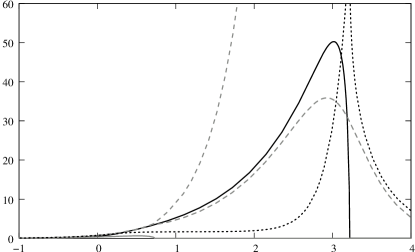
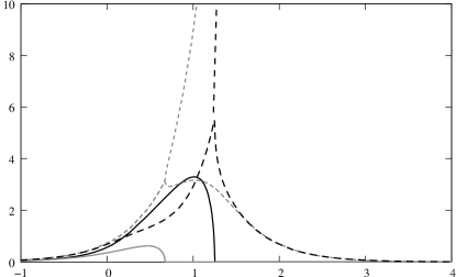
Figure 1: Dispersion curves for the illustrative parameter set: $v_{\rm A}=2\times 10^{-5}c$, $n_{\rm b}=n_{\rm p}/3$, $\Gamma_{\rm b}=10$ for two temperatures: $\Theta_{\rm p}=10^{-1}$ (right panel) and $10^{-3}$ (left panel). The real part of the frequency of each mode is shown as a dashed line, the imaginary part as a solid line. The left(right)-handed waves are shown in grey(black).

3 Wave modes

For a cold background plasma, and for low frequency modes such that $\omega^{\prime}\approx-\Gamma_{\rm b}\beta_{\rm b}ck$ with $\left|\omega^{\prime}\right|\gg\left|\omega_{\rm cb}\right|$, one recovers from Eq. (13) a simple form analogous to that discussed by Bell [2]:

$$\omega^{2} = {v_{\rm A}^{2}\over c^{2}+v_{\rm A}^{2}}\left(c^{2}k^{2}+{\beta_{\rm b}\omega_{\rm pb}^{2}ck\over\varepsilon\omega_{\rm cb}}\right)$$ (15)

which gives a purely growing mode ($\textrm{Re}(\omega)=0$) for the right-handed polarisation $\varepsilon=-1$, provided the driving by the beam-induced current is sufficiently strong. For $v_{\rm A}\ll c$, the mode reaches a maximum growth rate

$$\textrm{Im}(\omega) = \frac{1}{2}\frac{n_{\rm b}}{n_{\rm p}}\beta_{\rm b}\omega_{\rm pp}$$ (16)

which is independent of the magnetic field strength. The corresponding wave number is

$$k_{\rm max}=\frac{1}{2}\frac{n_{\rm b}}{n_{\rm p}}\beta_{\rm b}\frac{\omega_{\rm pp}}{v_{\rm A}}$$ (17)

The (non-resonant) thermal effects on this mode arising from the term containing $\left<u_{\bot}^{2}\right>$ are easily analysed in the case of weak magnetic field $v_{\rm A}\ll c$, since then $\omega^{2}\ll c^{2}k^{2}$ and $\omega^{\prime}\approx-\Gamma_{\rm b}\beta_{\rm b}ck$. The dispersion relation is then approximately

$$\tilde{\omega}^{2} = \frac{v_{\rm A}^{2}}{c^{2}}\tilde{k}\left(\tilde{k}+{\Gamma_{\rm b}\beta_{\rm b}^{2}\omega_{\rm pb}^{2}\over\varepsilon\omega_{\rm c}^{2}}-\tilde{k}{\left<u_{\bot}^{2}\right>\omega_{\rm pp}^{2}\over\varepsilon\Gamma_{\rm b}\beta_{\rm b}\omega_{\rm c}^{2}}\tilde{\omega}\right)$$ (18)

where dimensionless units are used in which $\tilde{k}=\Gamma_{\rm b}\beta_{\rm b}ck/\omega_{\rm c}$ and $\tilde{\omega}=\Gamma_{\rm b}\beta_{\rm b}\omega/\omega_{\rm c}$. The $\varepsilon=-1$ mode reaches a maximum growth rate of

$$\textrm{Im}(\omega) = \frac{\sqrt{3}}{2}\left(\frac{n_{\rm b}}{n_{\rm p}}\right)^{2\over 3}\left(\frac{v_{\rm A}}{c}\right)^{2\over 3}\left(\frac{\omega_{\rm pp}}{\omega_{\rm c}}\right)^{2\over 3}\left(\frac{\beta_{\rm b}^{2}}{\left<u_{\bot}^{2}\right>}\right)^{1\over 3}\omega_{\rm c}$$ (19)

In terms of the dimensionless temperature $\Theta_{\rm p}$ of the background protons for the appropriately normalised Jüttner-Synge distribution

$$\left<u_{\bot}^{2}\right> = 16\Theta_{\rm p}^{2}\left[1+3(1+\Theta_{\rm p})\right]\textrm{e}^{-1/\Theta_{\rm p}}/\left[K_{2}\left(1/\Theta_{\rm p}\right)\right]$$ (20)

so that the growth rate given by Eq. (19) falls off rapidly with increasing temperature.

After multiplication by the factor $\epsilon\omega_{\rm c}-\omega^{\prime}$, Eq. (1) together with Eq. (13) gives the dispersion relation as a fourth order polynomial in $\omega$ with real coefficients. Keeping all terms in this expression, which is valid for wavenumbers $\left|\hat{k}\right|\ll\Gamma_{\rm b}\beta_{\rm b}/\Theta$, far from resonance with the background protons, the low frequency modes are shown in Fig. 1.

4 Discussion

From Fig. 1 it can be seen that the $\varepsilon=1$ mode (grey curves) resonates with the beam particles when $k$ is close to their inverse gyro-radius, i.e., $\hat{k}\approx 1$. This is the cyclotron resonant mode considered by, amongst others, Pohl & Schlickeiser [15]. However, for low to moderate values of the background temperature, its growth rate is very much slower than that of the non-resonant, current-driven mode (black curves). Near the peak of the unstable band of the non-resonant mode, the waves are strongly modified by the beam and do not resemble Alfvén waves: the phase velocity of the non-resonant mode is lower than that of the resonant mode, and both speeds generally exceed $v_{\rm A}$ substantially. At very large wavelengths, the modes converge and become Alfvén waves. This also happens for large $k$ values outside the unstable band, but only if these do not resonate with the background protons.

Eqs (16) and (17), show that in a cold background with $n_{\rm b}\approx n_{\rm p}$, the non-resonant mode has a maximum growth rate comparable to that of electrostatic oscillations, although at much shorter (parallel) wavelengths. Only a relatively modest temperature $\Theta_{\rm p}\approx\omega_{\rm c}/\omega_{\rm pp}$ suffices to damp such waves, as can be seen from Eq. (19). Physically, this can be understood by noting that, as the background temperature rises, an increasing number of particles react to the wave perturbation as if they were unmagnetized. This reduces the effective current driving the instability. Ultimately, if all particles react in the same way to the perturbation (i.e., all are magnetized or all are unmagnetized) the plasma behaves as a fully compensated system with no driving current. Eq. (19) also shows that, for fixed temperature, the growth rate scales with the cyclotron frequency of the background protons. For $\Theta_{\rm p}\approx 1$ and $n_{\rm b}\approx n_{\rm p}$, the maximum growth rate is approximately equal to $\omega_{\rm c}$.

The crucial question of the nonlinear evolution of the system has been discussed in the nonrelativistic case by Bell [2] and Milosavljević & Nakar [12]. Saturation can be expected when the currents associated with the growing waves become comparable to the current induced by the beam. Applying this to the relativistic case, one finds for the amplitude $B_{\rm w}$ of the magnetic field of the perturbations

$$\left|\vec{k}\wedge\vec{B}_{\rm w}\right|\approx q_{\rm b}n_{\rm b}c\beta$$ (21)

If we assume that the largest wavelength in our system is of the order of the gyroradius of the beam protons, we can estimate the maximum magnetic field energy density to be

$${B_{\rm w}^{2}\over 8\pi}\approx\frac{1}{2}n_{\rm b}\Gamma m_{\rm p}c^{2}$$ (22)

This suggests that the entire energy content of the beam is, at least initially, transferred into transverse field fluctuations. The efficiency of magnetic field generation by this mechanism (i.e., the ratio of the saturated field energy density to that in the incoming stream) is somewhat higher than that attributed to the Weibel instability in the case of a relativistic shock in a pair plasma [18]. The Weibel instability is not thought to be effective in mediating shocks in electron/proton plasmas [9]. However, the efficacy of the instability described here depends strongly on the ability of the plasma to convert the energy input at small scales into a larger scale magnetic field.

Acknowledgements

This research was jointly supported by Cosmogrid and the Max-Planck-Institut für Kernphysik.

References

References

- [1] A. Achterberg, Astronomy & Astrophysics 119, 274 (1983)
- [2] A.R. Bell, Mon. Not. R. Astron. Soc. 353, 550 (2004)
- [3] A.R. Bell, Mon. Not. R. Astron. Soc. 358, 181 (2005)
- [4] A.R. Bell, S.G. Lucek, Mon. Not. R. Astron. Soc. 321, 433 (2001)
- [5] R. Blandford, D. Eichler, Physics Reports, 154, 1, 1 (1987)
- [6] L. O’C. Drury, Rep. Prog. Phys., 46, 973 (1983)
- [7] C.B. Hededal, K.-I. Nishikawa, Astrophysical Journal, 623, L89 (2005)
- [8] F. Jones, D. Ellison, 58, 259, (1991)
- [9] Y. Lyubarsky, D. Eichler, Astrophysical Journal, 647,1250 (2006)
- [10] J.F. McKenzie, H.J. Völk, Astronomy & Astrophysics 116, 191 (1982)
- [11] M.V. Medvedev, A. Loeb, Astrophysical Journal, 526,697 (1999)
- [12] M. Milosavljević, E. Nakar, astro-ph/0512548 (2005)
- [13] K.-I. Nishikawa, P. Hardee, G. Richardson, R. Preece, H. Sol, G.J. Fishman, Astrophysical Journal, 595, 555 (2003)
- [14] T. Piran, Rev.Mod.Phys. 76, 1143 (2004)
- [15] M. Pohl, R. Schlickeiser, Astronomy & Astrophysics 354, 395 (2000)
- [16] M. Pohl, I. Lerche, R. Schlickeiser, Astronomy & Astrophysics 383, 309 (2002)
- [17] L.O. Silva, R.A. Fonseca, J.W. Tonge, J.M. Dawson, W.B. Mori, M.V. Medvedev, Astrophysical Journal, 596, L121 (2003)
- [18] A. Spitkovsky, 2005AIPC, 801, 345S, (2005)
- [19] J. Wiersma, A. Achterberg, Astronomy & Astrophysics 428, 365 (2004)
- [20] P.H. Yoon, Phys. Fluids B. 2, 4, (1990)