The nuclear regions of NGC 7582 from [Ne II] spectroscopy
at 12.8$\mu$m – an estimate of the black hole mass

We present a high-resolution ($R\approx 16,000$) spectrum and a narrow-band image centered on the [Ne ii]12.8 $\mu$m line of the central kpc region of the starburst/Seyfert 2 galaxy NGC 7582. The galaxy has a rotating circum-nuclear starburst disk, shown at great detail at a diffraction-limited resolution of 0$\aas@@fstack{\prime\prime}$4 ($\approx 40$ pc). The high spatial resolution allows us to probe the dynamics of the [Ne ii] gas in the nuclear regions, and to estimate the mass of the central black hole. We construct models of gas disks rotating in the combined gravitational potential from the stellar bulge and a central black hole, and derive a black hole mass of $5.5\times 10^{7}$ M_⊙ with a 95% confidence interval of [3.6,8.1]$\times$10⁷ M_⊙. The black hole mass combined with stellar velocity dispersion measurements from the literature shows that the galaxy is consistent with the local $M_{\rm BH}$-$\sigma_{*}$ relation. This is the first time that a black hole mass in a galaxy except our own Milky Way system has been estimated from gas dynamics in the mid-infrared. We show that spatially resolved mid-infrared spectroscopy may be competitive with similar techniques in the optical and near-infrared, and may prove to be important for estimating black hole masses in galaxies with strong nuclear dust obscuration. The high spectral resolution allows us to determine the heliocentric systemic velocity of the galaxy to between 1614 and 1634 km s^-1. The mid-infrared image reveals several dense knots of dust-embedded star formation in the circum-nuclear disk, and we briefly discuss its morphology.

1 Introduction

Much effort is currently being put into understanding how black holes form and grow in the context of galaxy formation (e.g. Haehnelt & Kauffmann 2000; Marconi et al. 2004; Di Matteo et al. 2005; Cattaneo et al. 2005). The $M_{\rm BH}$–$\sigma_{*}$ relation (Ferrarese & Merritt 2000; Gebhardt et al. 2000), being a tight correlation between black hole mass and stellar velocity dispersion, is strong evidence for a causal link between the growth of the black hole and the galaxy bulge. The $M_{\rm BH}$–$\sigma_{*}$ relation has become our most important tool for studying the co-evolution of black holes and galaxies. To advance our knowledge we need to investigate how black hole mass and bulge velocity dispersion relate in a variety of galaxies, over a wide range in Hubble type, black hole mass and velocity dispersion. However, direct measurements of black hole mass in galaxies are challenging because resolutions of the order of the radius of the sphere of influence of the black hole are required, a scale which is typically $\ll 1\arcsec$.

A widely used method for black hole mass measurement is that of spatially resolved spectroscopy of rotating gas disks in the centers of nearby galaxies. Because spatial resolutions of typically 0$\aas@@fstack{\prime\prime}$1 are needed, this method has mainly utilized the Hubble Space Telescope (HST) (e.g. Ferrarese et al. 1996; van der Marel & van den Bosch 1998; Verdoes Kleijn et al. 2000; Barth et al. 2001; Marconi et al. 2003; Atkinson et al. 2005). With the superior resolution of the HST, gas rotation close to, or inside, the black hole’s sphere of influence, i.e. inside which the black hole potential dominates over the bulge potential, can be measured. For the more massive black holes, say $>10^{8}$ M_⊙, or for sufficiently nearby galaxies, the sphere of influence can also be resolved from the ground at near-infrared wavelengths (e.g. Marconi et al. 2001; Tadhunter et al. 2003).

Now that the Space Telescope Imaging Spectrograph (STIS) on board HST is no longer operational, it becomes necessary to find alternative techniques with sufficient spatial resolution to probe dynamics of gas and stars close to the black hole’s sphere of influence. Adaptive optics assisted spectroscopy in the near-infrared is the most obvious alternative because resolutions of $<0\aas@@fstack{\prime\prime}1$ can routinely be reached (Häring-Neumayer et al. 2006). Here we show that also diffraction limited spectroscopic imaging in the mid-infrared at 8m class telescopes is a viable technique.

Some galaxies have nuclei that are hidden behind large amounts of dust, hence the nuclear regions become unavailable at optical, and sometimes also at near-infrared, wavelengths. However, the dust is penetrated at mid-infrared wavelengths, and mid-infrared spectroscopy at high spatial resolution can therefore be used to constrain black hole masses in dust enshrouded galaxy nuclei. The starburst/Seyfert 2 galaxy NGC 7582 is an example of a such a galaxy. Here we present data of this galaxy taken with the ESO mid-infrared instrument VISIR (VLT Imager and Spectrometer for mid-InfraRed). The data consist of a narrow-band image and two high-resolution long-slit spectra centered on the [Ne ii]12.8$\mu$m line.

NGC 7582 is a highly inclined barred spiral galaxy (SBab) at a systemic velocity $cz\approx 1620$ km s^-1 with a composite starburst/Seyfert 2 nucleus. The nucleus has a well-defined one-sided ionization cone in [O iii]5007 (Storchi-Bergmann & Bonatto 1991). In the center, there is circum-nuclear H$\alpha$ emission distributed in a rotating kpc-scale disk in the plane of the galaxy, perpendicular to the cone axis (Morris et al. 1985). The nucleus is hidden behind large amounts of dust (Regan & Mulchaey 1999), presumably associated with the putative torus.

The starburst in the center is associated with the nuclear kpc-scale disk seen in low-excitation emission lines (Morris et al. 1985; Sosa-Brito et al. 2001) and in the soft X-rays, extended emission from the starburst is seen (Levenson et al. 2001). Low-resolution spectra and images in the mid-infrared show PAH (Polycyclic Aromatic Hydrocarbon) emission from star forming regions (Siebenmorgen et al. 2004). The nuclear AGN (Active Galactic Nucleus) point source is strong and well-defined in the $L$ (3.8$\mu$m) and $M$ (4.7$\mu$m) bands, and the star forming kpc-scale disk also shows up in the $L$-band image (Prieto et al. 2002), probably because of PAH emission at 3.3$\mu$m. Near-infrared spectra show both broad and narrow Br$\gamma$ (Reunanen et al. 2003). Wold & Galliano (2006) discuss the star formation in the disk in more detail, in particular the presence of embedded star clusters discovered in the [Ne ii] narrow-band image, with no counterparts detected at optical or near-infrared wavelengths. They estimate that the two brightest sources in the disk may contain roughly 1500 O stars each, and are likely to be young, super star clusters embedded in their own dusty birth material.

Throughout the paper, a Hubble constant of $H_{0}=70$ km s^-1 Mpc^-1 is used, hence one arcsec corresponds to $\approx 108$ pc in the rest-frame of the galaxy.

2 Observations and data reduction

A narrow-band image and two long-slit spectra were obtained with the VISIR instrument mounted at the Cassegrain focus of the UT3 Melipal telescope. The VISIR detector is a SiAs 256$\times$256 DRS array, and the pixel scale used during the observations was 0$\aas@@fstack{\prime\prime}$127, yielding a field of view of 32$\aas@@fstack{\prime\prime}$5$\times$32$\aas@@fstack{\prime\prime}$5.

The image was taken on 2004 September 29 through the [Ne ii] narrow-band filter centered on 12.81$\mu$m (half-band width 0.21$\mu$m). A perpendicular chopping-nodding technique was used with a chop throw of 12$\aas@@fstack{\prime\prime}$0 and a total integration time of one hour. The two high-resolution spectra were obtained on October 2 using the [Ne ii]12.8$\mu$m long-slit echelle mode. Both spectra are centered on the nucleus. One spectrum was obtained with the slit approximately parallel to the major axis of the circum-nuclear disk and the other with the slit perpendicular to the major axis. A parallel chop-nod technique was used with nodding along the slit. The chop throw amplitude was 12$\aas@@fstack{\prime\prime}$0 and the total integration time for each spectrum was one hour.

The spectra were obtained with the 0$\aas@@fstack{\prime\prime}$75 slit and the grating tilted to a central wavelength of 12.8803$\mu$m. With this setting, the dispersion is 1.372$\times$10${}^{-4}\mu$m per pixel, and the resolving power $R\approx 16000$. For calibrations, a telluric standard star, HD1522, with spectral type K1.5III, was observed. Conditions on both nights were clear with humidity below 10%.

The PSF in the narrow-band image has a FWHM (Full Width at Half Maximum) of 0$\aas@@fstack{\prime\prime}$4. The spatial resolution in the spectrum is also 0$\aas@@fstack{\prime\prime}$4, hence the data are diffraction limited as the diffraction limit for the VLT is 0$\aas@@fstack{\prime\prime}$39 at 12.8$\mu$m. The spectral resolution is given by the width of the function which is a convolution of the Line Spread Function (LSF) and the slit function. If we assume that the slit function is a rectangular function with width equal to the slit width of 5.9 pixels, and convolve it with a Gaussian LSF with a FWHM of 4 pixels, we obtain a profile with a width of $\approx 7$ pixels, corresponding to the FWHM of sky lines in the spectra. The LSF can therefore be approximated by a Gaussian with a FWHM of 4 pixels, implying that the instrumental broadening (FWHM) is 4 pixels, or $\approx 13$ km/s.

Pipeline-reduced images and spectra are used throughout the paper. For each telescope nodding position the average of all chopped frames is built and the different nodding frames are combined to derive the final image. The wavelength calibration is performed by cross-correlating the position of skylines in the observed spectrum with that of a HITRAN spectrum (Rothman et al. 2003). The pipeline wavelength calibration was checked by identifying the three strongest skylines with the corresponding skylines in high resolution ($R\approx 130,000$) $N$-band solar spectra from the McMath Fourier Transform Spectrometer (Wallace et al. 1994), and an agreement to within less than two pixels was found.

3 The circum-nuclear star forming disk

In order to study the structure of the circum-nuclear disk, we formed a color image of the central $\sim 10\arcsec\times 10\arcsec$ by combining the VISIR narrow-band image with archival HST WFPC2 and NICMOS images taken through the $F606W$ and $F160W$ filters (programmes 8597 and 7330, respectively). The NICMOS image was obtained with the NIC2 detector, and for the WFPC2 image, we used only the PC chip covering the nucleus. The colour image is shown in Fig. 1 where the WFPC2 image has been coded in blue, the NICMOS image ($H$-band) in green and the [Ne ii] narrow-band image in red. The image agrees well with the model favoured by Morris et al. (1985) based on observations of [O iii] and H$\alpha$. They suggest a rotating, star forming kpc-scale disk surrounding the nucleus with a one-sided outflowing ionization cone with the axis perpendicular to the disk plane.

There is a striking anti-correlation between the three colors in the image. The blue-coded optical emission dominated by the stellar continuum is obscured by a dust band stretching across the nucleus from the South-East towards the North-West. Since there is some contribution from H$\alpha$ to the optical flux the cone-structure can be seen in blue at $PA\approx 250\degr$ opening up towards the West. The green-coded near-infrared emission coming mainly from stars in the circum-nuclear disk is seen through the dust where the optical emission is obscured. But even the near-infrared emission is patchy because of dust obscuration, and in regions where both the near-infrared and optical emission has been extinguished by dust, the red-coded mid-infrared emission peeks through.

Figure 1: Color composite of the central kpc. The optical WFPC2 $F606W$ image is coded as blue and the near-infrared NICMOS $F160W$ image as green. The narrow-band image centered on the [Ne ii]12.8$\mu$m line is coded in red. North is up and East is to the left.

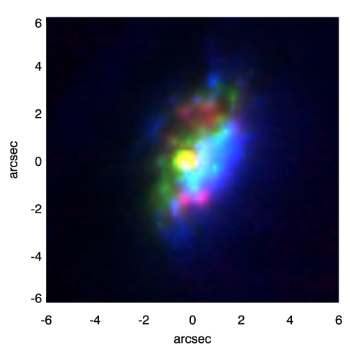
[Ne ii] is collisionally excited and the 12.8$\mu$m emission traces gas that has been ionized by UV radiation from newly formed, massive stars. Several knots of emission are seen, associated with dense, embedded regions of star formation. Wold & Galliano (2006) discuss the possibility that the bright [Ne ii] knots may be young star clusters consisting of $\sim 10^{3}$ stars, embedded in dusty material. The two most prominent knots are seen to the South of the nucleus. The rightmost knot is seen in the deconvolved 11.9$\mu$m image (tracing PAH emission) by Siebenmorgen et al. (2004), but the one to the left is undetected at 11.9$\mu$m. It is also very weak, or undetected, in H₂ (Sosa-Brito et al. 2001).

Using isophotal ellipse fitting, we measure the ellipticity and position angle of the [Neii] disk after masking out the knots. The best measurements at a semi-major axis of $\approx$ 2$\aas@@fstack{\prime\prime}$5 give an ellipticity of $0.47\pm 0.11$ and a position angle of $158\degr\pm 4\degr$. Assuming a thin, circular disk, the inclination angle is given by $\cos i=\frac{b}{a}$, implying that $i=58\degr$. The circum-nuclear gas disk therefore has, within the errors, the same inclination angle as the galaxy, $60\degr\pm 10\degr$ (Morris et al. 1985), and is consistent with lying in the plane of the galaxy. The rotation of the disk follows the direction of rotation of the galaxy.

4 The velocity field in the disk

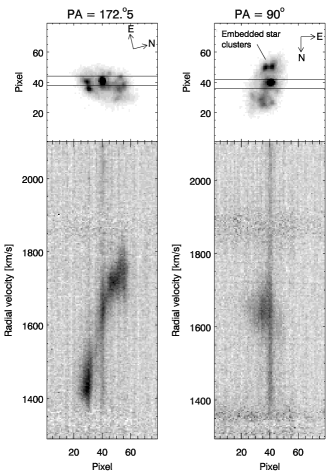
The two [Ne ii] longslit spectra show the velocity field across the disk along two directions almost perpendicular to each other. Fig. 2 shows the full two-dimensional spectra together with the narrow-band image with slit positions indicated. The parallel spectrum (shown to the left) was taken with the slit positioned over the nucleus and one of the compact knots of [Ne ii] emission to the South. The position angle is $PA=172\aas@@fstack{\circ}5$, which is close to the position angle of the major axis of the disk. The perpendicular spectrum, shown in the right-hand panel, was obtained at $PA=90\degr$, i.e. along the axis of the ionization cone. Both spectra show continuum emission from hot dust in the centre. The parallel spectrum clearly exhibits rotation, whereas the velocity across the minor axis as seen in the perpendicular spectrum is roughly constant.

Figure 2: The two high-resolution spectra of the [Ne ii] line with the slit positions indicated on the narrow-band image. The parallel spectrum is shown to the left, and the perpendicular spectrum to the right. The two regions of increased noise at $\approx 1350$ and 1850 km s^-1 are due to strong skylines. Continuum from hot dust emission in the center is seen.

Figure 3: Radial velocity, velocity dispersion and flux of the [Ne ii] line as a function of position along the slit in the two spectra. The panels to the left show the parallel spectrum, and the panels to the right, the perpendicular spectrum.

In order to derive velocity curves, apertures two pixels wide were extracted from the spectra. A Gaussian was fitted to each extracted spectrum so that the line centroid, FWHM and flux as a function of position along the slit could be determined. The results are shown in Fig. 3 where wavelength has been converted to radial velocity and FWHM to velocity dispersion (FWHM/2.35).

The parallel chop-nod technique produces one positive and two negative images on the detector. The positive image contains half of the total flux and each of the two negative images, a quarter of the total flux. As we were concerned with determining the position of the wavelength centroid as accurately as possible we chose not to combine the three spectral images, as imperfect registration could have introduced centroid shifts. Averaging the three images also does not increase the signal-to-noise by more than a factor of $2/\sqrt{3}$ (because each image contains only part of the total flux).

The data shown in Fig. 3 were extracted from the positive spectrum which has the highest signal-to-noise. For estimating uncertainties in wavelength centroid, FWHM and line flux, we utilized both the positive and the two negative spectra. The uncertainty in each quantity $x$, where $x$ may be line centroid, FWHM or flux, was calculated as $(|x_{\rm pos}-\bar{x}_{\rm neg}|)/2$, where $\bar{x}_{\rm neg}$ is the average of the measurements from the two negative images and $x_{\rm pos}$ is measured from the positive image. We find an uncertainty in the wavelength centroid of typically 5–10 km s^-1, depending somewhat on the position along the slit. There is an additional uncertainty due to the fact that the spatial resolution in the spectrum is smaller than the slit width. However, this is a systematic offset which does not vary with wavelength, hence was not taken into account here. The uncertainty in the velocity dispersion is 3–7 km s^-1 and the uncertainty in the flux, from a few up to $\approx 10$ per cent.

The rotation curve in the upper left-hand panel of Fig. 3 shows that the disk rotates with an amplitude of $\approx 200$ km s^-1. The rotation curve also appears relatively smooth with some irregularities close to the edges. In the blueshifted southern part of the disk (over pixels 26–38) a slight turn-over in the velocity is observed, probably indicating that most of the mass probed by the rotation curve is contained in the probed region. The rotation of the disk is such that the emission to the North is redshifted and the emission to the South blueshifted.

The perpendicular velocity curve to the right shows a more constant velocity of $\approx 1650$ km s^-1 across the disk with a slight decrease in velocity toward the East. An approximately constant velocity profile is what we expect from a perpendicular spectrum aligned along the minor axis of a thin rotating disk.

The middle row of panels in Fig. 3 shows velocity dispersion as a function of position along the slit. Typically we measure dispersions of 40–80 km s^-1 with maximum around the center of the disk. There are several different factors contributing to the velocity dispersion. Apart from unresolved rotation, there are contributions from instrumental and thermal broadening. The instrumental broadening is $\approx 13$ km s^-1 (see Section 2), and the thermal broadening broadening (FWHM) for a $10^{4}$ K disk $\approx 20$–30 km s^-1. This adds up to a FWHM of $\approx 24$–33 km s^-1, or $\sigma\approx 10$–14 km s^-1. We measure $\sigma>40$ km s^-1 so there must be a non-negligible contribution from bulk motion in the gas. The increase in velocity dispersion toward the center of the disk is seen in both the parallel and the perpendicular spectrum, probably caused by spatially unresolved rapidly rotating gas close to the nucleus.

The radius of the black hole sphere of influence is $GM_{\rm BH}/\sigma_{*}^{2}$ where $M_{\rm BH}$ is the black hole mass and $\sigma_{*}$ is the central stellar velocity dispersion. The velocity dispersion of NGC 7582 listed in the HyperLeda database is 157$\pm$20 km/s, and using aperture corrections by Jørgensen et al. (1995) and the $M_{\rm BH}-\sigma_{*}$ relation by Tremaine et al. (2002), we estimate a black hole mass of $\approx 4\times 10^{7}M_{\sun}$. Hence the radius of the black hole sphere of influence is $\la$ 0$\aas@@fstack{\prime\prime}$1. The spatial resolution in the [Ne ii] spectrum is a factor of 3–4 larger than this, so the sphere of influence is unresolved. But even though the spatial resolution is not sufficient to probe gas rotation inside the sphere of influence, an estimate of the black hole mass can be obtained from the steepness of the rotation curve across the nucleus. In the following, we set up a model of the rotating disk to be able to estimate the central black hole mass. Our modeling follows largely that of Barth et al. (2001), and is the standard gas-dynamical method used for nuclear gas disks in galaxies (see also Marconi et al. 2001; Tadhunter et al. 2003; Atkinson et al. 2005). The gas disk is assumed to rotate in the combined potential of the galaxy bulge and the central supermassive black hole. By varying the black hole mass as well as other parameters such as disk inclination and mass-to-light ratio, different models can be compared to the data in order to find the best fit. We describe the modeling in more detail in the following section.

5 The model velocity field

5.1 The basic equations

We assume that the circum-nuclear disk can be approximated by a flat, circular disk with constant inclination rotating in the gravitational potential $\Psi$. At every radius $R$ in the disk, the rotation is dictated by a combination of the gravitational potential from the stellar bulge and the central, supermassive black hole,

$$\Psi(R)=\Psi_{*}(R)+\frac{GM_{\rm BH}}{R}.$$ (1)

The bulge potential is $\Psi_{*}$ and the black hole point mass potential is $GM_{\rm BH}/R$. The bulge potential dominates far out in the disk, but close to the center, within the black hole sphere of influence, there is a non-negligible contribution from the black hole. The circular velocity, $v_{\rm c}$, in the disk is obtained by differentiating the potential with respect to $R$:

$$v_{\rm c}^{2}(R)=R\frac{\partial{\Psi}}{\partial{R}}.$$ (2)

The plane of the sky is defined by the coordinate system $(x^{\prime},y^{\prime})$ where the $x^{\prime}$-axis coincides with the major axis of the disk. We also define the slit coordinate system $(x_{\rm s},y_{\rm s})$ with the $y_{\rm s}$-axis along the length of the slit. The transformation between the two coordinate systems is given by

$$x^{\prime} = (x_{\rm s}-b)\sin\theta+y_{\rm s}\cos\theta$$

$$y^{\prime} = -(x_{\rm s}-b)\cos\theta+y_{\rm s}\sin\theta$$ (3)

(see appendix B by Marconi et al. 2001), where $\theta$ is the angle between the slit and the major axis of the disk. In our case, the slit is rotated by $\theta=-14\aas@@fstack{\circ}1$ with respect to the major axis (i.e. 158$\aas@@fstack{\circ}$4, which is the position angle of the disk, minus the slit position angle of 172$\aas@@fstack{\circ}$5). The center of the disk, i.e. the dynamical center, is assumed to have coordinates $x_{\rm s}=b$ and $y_{\rm s}=0$, hence the $b$-parameter enables us to take into account that the dynamical center may not be at the exact center of the slit.

The inclination of the disk is $i$, and we have by deprojection that

$$R^{2}=x^{\prime 2}+\left(\frac{y^{\prime}}{\cos i}\right)^{2}.$$ (4)

The velocity along the line of sight is given by

$$v=v_{\rm c}\sin i\frac{x^{\prime}}{R}.$$ (5)

From the equations above, we calculate the velocity along the line of sight in the slit coordinate system for any combination of bulge potential, black hole mass, disk inclination and dynamical center position $b$. By comparing the velocity curves derived from the different models to the observed one, the best-fitting parameters, including black hole mass, can be found.

5.2 The bulge gravitational potential

An important part of setting up the model is to determine the bulge gravitational potential, $\Psi_{*}(R)$. In order to do this, we use the stellar density in the bulge as a tracer of the gravitational potential. The NICMOS $F160W$ image is well suited for this because the near-infrared is a good tracer of stellar mass and because the image has high spatial resolution. Moreover, near-infrared is less affected by dust than the optical, a clear advantage here because the center of NGC 7582 is strongly affected by dust.

In order to parameterize the surface brightness distribution, we use the Multi-Gaussian Expansion (MGE) method developed by Cappellari (2002). It consists of parameterizing the galaxy surface brightness with a series expansion of two-dimensional Gaussian functions which can be converted to a gravitational potential $\Psi_{*}$. But since even the $F160W$-band is affected by dust, we found it necessary to make a correction before applying the MGE analysis to the image. This was done by mapping the extinction across the central parts of the galaxy by forming an $F606W-F160W$ image. The absolute extinction in the $F160W$-band was thereafter calculated by assuming a galactic reddening law (Cardelli et al. 1989) and a correctly-normalized dust-corrected image made by matching pixels in the uncorrected image to pixels in the corrected image that appeared unreddened. For simplicity, we assume a uniform intrinsic colour in the bulge, but in reality a gradient may exist.

In order to avoid introducing too many distortions in the surface brightness profile, the dust lane that runs across the galaxy was masked out before performing the MGE fit. The parameters of the best fit is listed in Table 1, where each Gaussian is characterized by a surface density $I_{k}^{\prime}$, a dispersion $\sigma_{k}^{\prime}$, and an axial ratio $q_{k}^{\prime}$. The luminosity $L_{k}$ in the last column is the total luminosity of the Gaussian. Primed quantities are projected whereas unprimed quantities are intrinsic. The luminosity $L_{k}$ is calculated as $2\pi I^{\prime}_{k}q_{k}^{\prime}\sigma_{k}$, where we have assumed that the gravitational potential is axissymmetric so that $\sigma_{k}^{\prime}=\sigma_{k}$.

In order to take the shape of the NICMOS PSF into account in the MGE analysis, we also computed a TinyTim PSF (Krist & Hook 1997) and parameterized it with four circular Gaussians (Cappellari 2002):

$${\rm PSF}(R^{\prime})=\sum_{k=1}^{M}G_{k}\exp[-R^{\prime 2}/(2\sigma_{k}^{*2})]/(2\pi\sigma_{k}^{*2}),$$ (6)

where $\sigma^{*}_{k}$ are the dispersions and $G_{k}$ the weights of the Gaussians. The parameters of the MGE fit to the NICMOS PSF are listed in Table 2.

The gravitational potential corresponding to an MGE density profile in the oblate axissymmetric case is given by

$$\Psi_{*}(R,z=0)=G\Upsilon\sqrt{\frac{2}{\pi}}\sum_{k=0}^{N}\frac{L_{k}\ \cal Q_{k}(R,z=0)}{\sigma_{k}}$$ (7)

(Emsellem et al. 1994; Cappellari et al. 2002), where $\Upsilon$ is the stellar mass-to-light ratio. The radius in the equatorial plane is $R$ and $z=0$ because the circular velocity in the equatorial plane is determined solely by the radial component of the force. We assume that the gas disk lies in the equatorial plane of the galaxy, hence the radial velocities we derive also lie in this plane. The factor $\cal Q_{k}$ is defined as

$$\cal Q_{k}(R,z=0)=\int_{0}^{1}\frac{\exp(-R^{2}T^{2}/2\sigma_{k}^{2})}{\sqrt{1-(1-q_{k}^{2})T^{2}}}{\rm d}T,$$ (8)

(see Cappellari 2002) where $q_{k}$ is the intrinsic axial ratio, calculated under the assumption that the galaxy has an inclination of 56$\aas@@fstack{\circ}$2, as measured by the MGE fitting routine.

Table 1: Parameters of the MGE fit to the galaxy bulge in the NICMOS F160W filter.

$k$	$I^{\prime}_{k}$	$\sigma^{\prime}_{k}$	$q^{\prime}_{k}$	$L_{k}$
	L⊙,F160W pc-2	arcsec		$10^{6}$ L⊙,F160W
1	33307	0.330	0.716	192.5
2	1041	1.333	0.872	119.5
3	4969	2.229	0.556	1018.5
4	343	7.188	0.556	730.2

Table 2: Parameters of the MGE fit to the NIC2 PSF in the F160W filter.

$k$	$G_{k}$	$\sigma_{k}^{*}$ [pix]
1	0.251	0.75
2	0.475	1.78
3	0.146	7.64
4	0.127	19.51

5.3 Generation of two-dimensional synthetic spectra

Having determined the bulge gravitational potential, we use the equations outlined in Section 5.1 to calculate models for different values of black hole mass and dynamical center offset, $b$. The disk inclination and the mass-to-light ratio are held constant at $i=58$° and $\Upsilon=3.8$ as the data do not have sufficient resolution to allow for a multi-parameter fit. The mass-to-light ratio is fit separately, prior to fitting $M_{\rm BH}$ and $b$, as explained in Section 5.4.

Each model is “observed” with the 0$\aas@@fstack{\prime\prime}$75 slit and the instrumental setup that was used during the observations. We also convolve with the resolution of the observations, and fold the [Ne ii] narrow-band image into the model in order to produce a two-dimensional synthetic spectrum. We follow the procedure of Barth et al. (2001), which is briefly described below. A detailed explanation can be found in Barth et al.’s paper.

First we set up a coordinate grid on which to compute the synthetic spectrum. The grid is subsampled by a factor of two compared to the data, so the pixel size in the model spectrum is half the size of the real pixels. The model is therefore resampled before comparing to the data. The construction of the synthetic spectrum consists of calculating the observed surface brightness of the disk through the 0$\aas@@fstack{\prime\prime}$75 slit. This is done by assuming that the intrinsic line profiles are Gaussians and adding them up at every point in the disk, weighing by the [Ne ii] surface brightness (as provided by the narrow-band image) and smearing by the seeing PSF.

The synthetic line profile, $f_{y_{\rm s}}(v)$, is given by Barth et al.’s (2001) eq. 4, and is reproduced here in order to clarify the discussion:

$$f_{y_{\rm s}}\left(v\right) = \sum_{x_{\rm s}=x_{0}}^{x_{1}}\sum_{i,j}S_{ij}P(i,j|x_{\rm s},y_{\rm s})$$ (9)

$$\times\exp\left[\frac{\left[v-v_{\rm p}(i,j)-(x_{\rm s}-x_{\rm c})v_{\rm d}\right]^{2}}{-2\sigma_{\rm r}^{2}}\right].$$

The [Ne ii] surface brightness in the disk at pixel $(i,j)$ on the model grid is denoted $S_{ij}$, and the value at $(x_{\rm s},y_{\rm s})$ of a PSF centered at pixel $(i,j)$ is denoted $P(i,j|x_{\rm s},y_{\rm s})$. Hence the multiplication of $S$ and $P$ represents a convolution of the surface brightness distribution with the PSF and takes into account that different parts of the disk contribute to the velocity profile at a given position. We assume that the PSF is a Gaussian with FWHM equal to the seeing. During the computations the PSF was truncated at $2.5\times$FWHM. Since we are effectively convolving the narrow-band image with the PSF, the narrow-band image first had to be deconvolved. This was achieved by block replicating the original image by a factor of two and deconvolving using the Multiwavelength Deconvolution Method (Starck & Murtagh 2002).

Since the intrinsic line profiles are assumed to be Gaussians, the exponential factor in Eq. 9 contains the model velocity field $v_{\rm p}(i,j)$ and a correction factor $(x_{\rm s}-x_{\rm c})v_{\rm d}$ taking into account the uncertainty in velocity caused by the fact that the recorded wavelength of a photon depends on where it enters the slit along the $x_{\rm s}$-axis. The pixel size in velocity units is $v_{\rm d}=3.2$ km s^-1, and the center of the slit is denoted $x_{c}$. The velocity dispersion of the gas, $\sigma_{\rm r}$, occurs in the denominator. As seen from Fig. 3 it varies significantly across the disk, hence is difficult to fit by a model. We therefore approximate $\sigma_{\rm r}$ with $\approx 55$ km s^-1 which is the average across the disk.

In order to avoid including continuum emission in the synthetic spectra, the narrow-band image was continuum subtracted before incorporating it into the model. Because it was obtained solely for the purpose of aiding with the determination of slit positions, images in the continuum filters bracketing the [Ne ii] line were not taken. We therefore subtract a continuum based on that measured in the spectrum instead, achieved by first scaling a point source to the continuum flux measured in the spectrum, and thereafter subtracting it from the image. Because the narrow-band image is folded into the model, the position of the slit relative to the narrow-band image had to be determined. This was done by first rotating the image so that the length of the slit was parallel to the y-axis of the rotated image, and thereafter collapsing the spectrum in the wavelength direction and matching it to the section of the image covered by the slit.

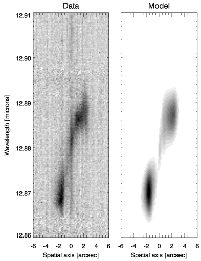
The summation over $x_{\rm s}$ in Eq. 9 runs across the width of the slit, where the edges of the slit are given by $x_{\rm s}=x_{0}$ and $x_{\rm s}=x_{1}$. The $y_{\rm s}$-coordinate runs along the spatial direction of the spectrum. To create the full two-dimensional spectrum, $f_{y_{\rm s}}(v)$ has to be evaluated for every pixel along the spatial direction. An example of a synthetic spectrum is shown in Fig. 4. The two regions of emission on either side of the center are well reproduced, as are their relative compactness and brightness. As the synthetic spectrum is noise free, and also void of sky lines, it differs slightly from the observed one, especially around $12.863\mu$m where there is increased noise due to the subtraction of a sky line. Also, since the synthetic spectrum was produced by convolving with a continuum-subtracted narrow-band image, the two differ in flux at the center.

Figure 4: Comparison between the real spectrum (left) and a synthetic spectrum (right), calculated for a black hole mass of $5.5\times 10^{7}$ M_⊙ and with the dynamic center shifted 0$\aas@@fstack{\prime\prime}$3 from the center of the slit.

In order to derive model rotation curves, we made extractions from the synthetic two-dimensional spectra in a manner identical to that which was done for the real spectrum.

5.4 Constraints on the black hole mass

Given that the VISIR spectrum has a spatial resolution of $\approx 0\aas@@fstack{\prime\prime}4$, we merely fit two parameters, namely the black hole mass and the location of the dynamical center within the slit. The inclination of the disk is fixed at $i=58\degr$ and the mass-to-light ratio at $\Upsilon=3.80$. We calculate models on a grid of black hole mass and dynamical center location, $b$. The spacing in $M_{\rm BH}$ was varied between 0.5$\times$10⁷ and 1$\times$10⁷ M_⊙, and the spacing in $b$, between 0$\aas@@fstack{\prime\prime}$1 and 0$\aas@@fstack{\prime\prime}$05, depending on how close the model was to the global minimum in $\chi^{2}$.

For every pair of $M_{\rm BH}$ and $b$ a synthetic two-dimensional spectrum was constructed, and one-dimensional spectra extracted from it using apertures of the same width as for the real data. Thereafter a Gaussian fit was made to each in order to determine the line centroid so that a radial velocity curve could be derived. The best-fitting model was found in a standard manner by minimizing $\chi^{2}$ between the observed and the model rotation curve. Fig. 5 shows the observed rotation curve together with a model rotation curve extracted from a synthetic spectrum.

In order to convert the MGE surface density profiles to a gravitational potential, the stellar mass-to-light ratio, $\Upsilon$, in the bulge has to be known, see Eq. 7. Outside the black hole’s sphere of influence, the rotation curve does not depend on either the black hole mass or the exact location of the dynamical center in the slit. Hence the outer parts of the rotation curve are not sensitive to $M_{\rm BH}$ and $b$, but depend instead on the mass-to-light ratio. We therefore fit $\Upsilon$ separately, before fitting $M_{\rm BH}$ and $b$, by neglecting the inner few points on the rotation curve and fitting only the outer parts. Synthetic spectra were generated with $M_{\rm BH}=0$ and $b=0$ and with mass-to-light ratios in the range 2.4–4.8 in steps of 0.2, while keeping the disk inclination constant at $i=58$°. Apertures were extracted and model rotation curves produced. The best-fit mass-to-light ratio was thereafter found by fitting the model rotation curves to the observed one with the three inner apertures (centered at pixels 36, 38 and 40) excluded. The best-fit model has $\Upsilon=3.80$ M_⊙/L_⊙ in the $F160W$ filter, in accordance with mass-to-light ratios observed in early-type spiral galaxies (Moriondo et al. 1998). We fix the mass-to-light ratio to 3.80 for the remainder of the fitting.

Upon comparing the model rotation curve to the observed one we have to decide on which aperture on the two curves should have the same radial velocity. Ideally, this corresponds to the point which has zero velocity in the rest frame of the galaxy, i.e. the point having radial velocity equal to the systemic velocity. However, because of the high spectral resolution of the VISIR data, the systemic velocity of NGC 7582 known from the literature is not accurate enough. Instead, we use the perpendicular spectrum to help constrain the radial velocity of the dynamical center. If the slit for the perpendicular spectrum is aligned along the minor axis of the disk, we expect to see a constant velocity along the slit corresponding to the systemic velocity. Examining the upper right-hand plot in Fig. 3, we see that there is a region over pixels 26–38 with constant velocity $\approx$1644 km s^-1. If this corresponds to the systemic velocity of the galaxy, then the aperture centered on pixel 40 in the parallel spectrum is the correct center to choose for the fitting because this is the aperture closest to 1644 km s^-1. However, if the region with velocity $\approx 1644$ km s^-1 in the perpendicular spectrum is affected by an outflow or some bulk motion, the center could have a lower radial velocity. The aperture centered on pixel 40 in the perpendicular spectrum has a velocity of 1632 km s^-1, and could therefore be closer to the dynamical center. Comparing again with the parallel spectrum, a velocity of 1632 km s^-1 lies between the apertures centered on pixels 38 and 40. So it is likely that the dynamical center in the parallel spectrum either coincides with one, or lies somewhere between these two apertures. The most probable systemic velocity of the galaxy therefore seems to be 1630–1650 km s^-1. Correcting to heliocentric velocity (the correction factor at the time of observation is $-$16 km s^-1), we therefore find that the systemic velocity of the galaxy is 1614–1634 km s^-1, approximately 60 km s^-1 higher than that reported in the Leda database based on optical emission lines. Outflows and bulk motion of the gas make it difficult to pin-point accurately the aperture corresponding to the systemic velocity. Integral field spectroscopy in the near-infrared might help in this respect, although even in this case, there may be problems related to dust obscuration and outflows.

By requiring that the observed and the modeled rotation curve have the same velocity in the aperture centered on pixel 38, we derive a best-fitting model with $M_{\rm BH}=1.0\times 10^{8}$ M_⊙ and $b=$0$\aas@@fstack{\prime\prime}$35 with a reduced $\chi^{2}$ of 3.76. By shifting the common aperture to the one centered on pixel 40, the fit is marginally better with a reduced $\chi^{2}$ of 3.36, $M_{\rm BH}=5.5\times 10^{7}$ M_⊙ and $b=$0$\aas@@fstack{\prime\prime}$3. The slightly different best-fit parameters in each case serves to illustrate the level of uncertainty related to the difficulties with knowing the exact systemic velocity. The reason we obtain a reduced $\chi^{2}$ greater than unity is most likely due to outflows and bulk motions in the gas that are not included in the model. The current modeling is probably the best that can be done with these data, and the limitations are due to uncertainties related to the spatial resolution being larger than the sphere of influence of the black hole.

We choose the model with $M_{\rm BH}=5.5\times 10^{7}$ M_⊙ as our best fit since this has the lowest $\chi^{2}$. This model is plotted together with the observed rotation curve in Fig. 5, and a contour plot of $\chi^{2}$ is shown in Fig. 6, with 68, 95% and 99% confidence regions indicated. The confidence regions on $M_{\rm BH}$ and $b$ are also listed in Table 3.

Figure 5: The open circles show the observed rotation curve and the solid line indicated the best-fit model with $M_{\rm BH}=5.5\times 10^{7}$ M_⊙ and $b=$0$\aas@@fstack{\prime\prime}$3. The dashed line corresponds to a model with $b=0.3$ and $M_{\rm BH}=0$.

Figure 6: Contours of $\chi^{2}$. The minimum is marked by an ’x’, and the solid lines mark the 68, 95 and 99% confidence regions.

Table 3: The confidence intervals for the parameters of the best-fitting model having $M_{\rm BH}=5.5\times 10^{7}$ M_⊙ and $b=$0$\aas@@fstack{\prime\prime}$3.

	$M_{\rm BH}$ [107 M⊙]	$b$ [arcsec]
68% CI	[3.2,8.7]	[0.282,0.341]
95% CI	[3.6,8.1]	[0.273,0.335]
99% CI	[4.4,7.1]	[0.294,0.314]

5.5 The dynamical center

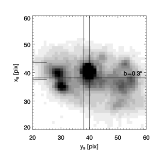
The best-fitting value $b=0\aas@@fstack{\prime\prime}3$ indicates that the dynamical center may not have been exactly centered on the slit when the spectrum was taken, but instead located 0$\aas@@fstack{\prime\prime}$085 from the edge of the slit, west of the center. We found above that the systemic velocity of the galaxy probably corresponds to the velocity probed by the apertures centered on pixel 38/40 in the parallel spectrum. These constraints can be used to find the location of the dynamical center on the narrow-band image, as shown in Fig. 7. In this figure, the image has been rotated so that the length of the slit runs horizontally, hence the abscissa is labeled $y_{\rm s}$. The ordinate is labeled $x_{\rm s}$ since it runs along the width of the slit. The location of the slit is indicated by the two short horizontal lines on the left-hand side of the image, and the line corresponding to $b=$0$\aas@@fstack{\prime\prime}$3 is the horizontal line plotted across the full width of the image. The two vertical lines correspond to the center of the two apertures that were discussed in the previous section as likely to correspond to the systemic velocity of the galaxy (between aperture 38 or 40). The dynamical center of the galaxy should therefore lie in the region where the horizontal line intersects the two vertical lines. As seen in Fig. 7, this region does not correspond to the exact location of the peak in the surface brightness, thereby suggesting that the dynamical center may be obscured.

Figure 7: The two shorter horizontal lines to the left indicate the slit width, and the two vertical lines the center of the two apertures thought to correspond to the systemic velocity of the galaxy. The horizontal line across the image indicates the best fit dynamical center position $b=0\aas@@fstack{\prime\prime}3$. The image has been rotated, so East is up and North is to the right. The axes are labeled according to the slit coordinate system.

According to unified models (Antonucci 1993), the location of the dynamical center is expected to coincide with the vertex of the ionization cone because the cone morphology is a result of the illumination of gas by the AGN continuum, which can only escape within $\pm\sim 45^{\circ}$ of the axis of the torus. The blue outline of the ionization cone is seen in the colour image in Fig. 1, but it is difficult to tell from the image precisely where the vertex is. The location of the dynamical center might therefore be consistent with the vertex of the cone.

6 Discussion

6.1 Black hole mass estimates in the mid-infrared

In order to prove the existence of a black hole or other compact object at the center of NGC 7582 with spatially resolved gas dynamics, the resolution must be sufficient to probe gas dynamics inside the black hole’s sphere of influence. The current data do not have the required spatial resolution for this, but if we accept that black hole activity is responsible for the AGN activity, the data presented here can be used to infer constraints on the mass of the black hole. We find a best-fitting black hole mass of 5.5$\times$10⁷ M_⊙, with a 95% confidence interval of [3.6,8.1]$\times$10⁷ M_⊙, consistent with the prediction of $\approx 4\times 10^{7}$ M_⊙ from the local $M_{\rm BH}$–$\sigma_{*}$ relation.

This is the first time that a black hole mass in a galaxy except our own Milky Way system has been estimated from gas dynamics using line emission in the mid-infrared. Usually H$\alpha$ and/or [N ii] in the optical have been used, in particular for HST data. Ground-based work has so far been limited to, and has relied on, emission lines in the near-infrared since better resolution is achieved at longer wavelengths. More measurements are expected to appear in the near-infrared with the application of adaptive optics (Häring-Neumayer et al. 2006). The VISIR data presented here are diffraction limited and therefore have the best obtainable spatial resolution possible with an 8-m telescope at the position of the [Ne ii] line. The black hole in NGC 7582 seems to be on the limit of what is possible to constrain with a spatial resolution of 0$\aas@@fstack{\prime\prime}$4, and probably black hole masses of $\ga 5$–$10\times 10^{7}$ M_⊙ in nearby galaxies with gas disks can be estimated from the ground using spectroscopy of the [Ne ii]12.8$\mu$m line.

Since dust is easily penetrated at mid-infrared wavelengths, gas dynamics in the mid-infrared may prove to be a valuable tool for probing the $M_{\rm BH}$–$\sigma_{*}$ relation in galaxies where the nuclear regions are obscured by dust and where optical and/or near-infrared spectroscopy may fall short. Gas dynamics in the mid-infrared may therefore help determine the black hole masses of e.g. Seyfert 2 galaxies where the nucleus is hidden behind an optically thick, dusty torus. The assumption is, as with optical and near-infrared observations, that the gas is well-behaved and has a relatively smooth rotation curve.

6.2 The morphology of the circum-nuclear disk

The two bright regions in the disk to the South of the nucleus may be dense regions of intense starformation, deeply embedded in dust (Wold & Galliano 2006). The two knots are equally bright in [Ne ii], but one of them is less bright, or undetected, in H₂ and at 11.9$\mu$m (Sosa-Brito et al. 2001; Siebenmorgen et al. 2004). Our modeling shows that the rotation curve of the disk, including the two bright knots to the South of the nucleus, is consistent with a thin disk rotating in the gravitational potential of the bulge. This suggests that the two knots lie in the plane of the disk. According to the unified model the ionization cone axis is perpendicular to the plane of the torus, and since the circum-nuclear disk is probably an extension of the torus, the two knots must be shielded from the ionizing continuum of the AGN. We therefore conclude that the AGN continuum cannot be responsible for the destruction of PAHs and H₂ in one of the knots. The lack of PAHs and H₂ in one knot relative to the other may be explained by differences in the ionizing continuum and/or by differences in the physical conditions in the molecular clouds. For instance, the PAH- and H₂-deficient knot may be further along in its lifetime and has ionized more of its local interstellar medium, destroying both PAHs and H₂ in the process. Alternatively, the PAH-deficient knot may contain a larger population of hot O-stars than the other since PAHs are found to be better tracers of B-star populations rather than very hot O-stars (Peeters et al. 2004). Finally, as PAHs and H₂ can arise in different regions and H₂ is very temperature-sensitive, differences in the physical conditions of the two knots may also influence their appearances.

7 Conclusions

We have presented data taken with the ESO VLT mid-infrared instrument, VISIR, consisting of a narrow-band image centered on the [Ne ii]12.8$\mu$m line, and two high-resolution ($R=16000$) spectra also centered on the [Ne ii] line, of the composite starburst-Seyfert 2 galaxy NGC 7582. The galaxy has a circum-nuclear star forming disk and the two long-slit spectra were obtained with the slit parallel and perpendicular to the major axis of the disk. The parallel spectrum shows a clear rotation curve, with an amplitude of $\approx 190$ km s^-1, and the perpendicular spectrum, a roughly constant velocity profile as expected for a geometrically thin disk.

We model the disk as a thin circular disk rotating in the combined gravitational potential of the bulge and a central black hole, and find a best-fit black hole mass of 5.5$\times$10⁷ M_⊙ with a 95% confidence interval of [3.6,8.1]$\times$10⁷ M_⊙. In the modeling we also allow for the fact that the dynamical center may not have been exactly at the center of the slit during observation. The best-fitting model indicates that it probably was located close to the edge of the slit, approximately 0$\aas@@fstack{\prime\prime}$3 to the west of the slit center. Taking advantage of the high spectral resolution, we argue that the (heliocentric) systemic velocity of the galaxy is $cz\approx 1614$–1634 km s^-1.

There are two dense starforming knots in the disk, equally bright in [Ne ii], but one shows weaker emission in H₂ and at 11.9$\mu$m, indicating that the PAHs and the H₂ may have been destroyed. Since the rotation in the outer parts of the disk, including the two knots, is well explained by a thin disk rotating in the gravitational potential of the bulge, we conclude that the two knots lie in the disk and are thereby shielded from the AGN continuum. If an ionizing continuum is responsible for the destruction of PAHs and H₂ in one of the knots, it must come from the star forming region itself rather than the AGN. It cannot be excluded however, that different physical conditions, e.g. temperature, within the two knots may be responsible for their different appearances in H₂ and at 11.9$\mu$m.

The data are diffraction limited with a spatial resolution of $\approx 0\aas@@fstack{\prime\prime}4$, and we argue that this resolution is sufficient to put constraints on black holes masses of $\ga 5$–$10\times 10^{7}$ M_⊙. Now that STIS on board HST is no longer operational, other techniques for estimating black hole masses in galaxies need to be explored. We have shown that gas dynamical estimates of black hole masses based on high-resolution mid-infrared spectroscopy are competitive with other techniques, particularly if the galaxy nucleus is obscured by dust. Such observations also allow us to study obscured star formation in the centers of nearby AGN, thus advancing our understanding of the connection between AGN activity and nuclear star formation.