Analysis and Interpretation of Hard X-ray Emission from the Bullet Cluster (1E0657-56), the Most Distant Cluster of Galaxies Observed by RXTE

Abstract

Evidence for non-thermal activity in clusters of galaxies is well established from radio observations of synchrotron emission by relativistic electrons. New windows in the Extreme Ultraviolet and Hard X-ray ranges have provided for more powerful tools for the investigation of this phenomenon. Detection of hard X-rays in the 20 to 100 keV range have been reported from several clusters of galaxies, notably from Coma and others. Based on these earlier observations we identified the relatively high redshift cluster 1E0657-56 (also known as RX J0658-5557) as a good candidate for hard X-ray observations. This cluster, also known as the bullet cluster, has many other interesting and unusual features, most notably that it is undergoing a merger, clearly visible in the X-ray images. Here we present results from a successful RXTE observations of this cluster. We summarize past observations and their theoretical interpretation which guided us in the selection process. We describe the new observations and present the constraints we can set on the flux and spectrum of the hard X-rays. Finally we discuss the constraints one can set on the characteristics of accelerated electrons which produce the hard X-rays and the radio radiation.

1 INTRODUCTION

The intra-cluster media (ICM) of several clusters of galaxies, in addition to the well studied thermal bremsstrahlung (TB) emission dominating in the $\sim 2-10$ keV soft X-ray (SXR) region, show growing evidence for non-thermal activity. This activity was first observed in a form of diffuse radio radiation (classified either as relic or halo sources). The first cluster with diffuse emission detected in the radio band was Coma, and recent systematic searches have identified more than 40 clusters with halo or relic sources. In the case of Coma, the radio spectrum may be represented by a broken power law (Rephaeli 1979), or a power law with a rapid steepening (Thierbach et al. 2003) or with an exponential cutoff (Schlickeiser et al. 1987). There is little doubt that this radiation is due to synchrotron emission by a population of relativistic electrons with similar spectra, however, from radio observations alone one cannot determine the energy of the electrons or the strength of the magnetic field. Additional observations or assumptions are required. Minimum total (particles plus field) energy or equipartition assumptions imply magnetic field strength of $B\sim\mu{\rm G}$, in rough agreement with the Faraday rotation measurements (e.g. Kim et al. 1990), and a population of relativistic electrons with Lorentz factor $\gamma\sim 10^{4}$. In the papers cited above, it was also realized that because the energy density of the Cosmic Microwave Background (CMB) radiation (temperature $T_{0}$) $u_{\rm CMB}=4\times 10^{-13}(T_{0}/2.8\,{\rm K})^{4}\,{\rm erg}\,{\rm cm}^{-3}$ is larger than the magnetic energy density $u_{\rm B}=3\times 10^{-14}(B/\mu{\rm G})^{2}\,{\rm erg}\,{\rm cm}^{-3}$, most of the energy of the relativistic electrons will be radiated via inverse Compton (IC) scattering of the CMB photons, producing a broad photon spectrum (similar to that observed in the radio band) around 50 keV (for $\gamma\sim 10^{4}$). Thus, one expects a higher flux of non-thermal X-ray radiation than radio radiation. Detection of HXRs would then break the degeneracy and allow determination of the magnetic field and the energy of the radiating electrons. Moreover, since the redshift dependence of the CMB photons is known, then in principle, the cosmological evolution of these quantities can also be investigated.

While the detectability of such radiation would be easiest in the soft X-ray range, where very sensitive imaging instruments are available, in reality, in this range, it is masked by the prominent thermal bremsstrahlung emission, a general characteristic of clusters. With this, the most promising is either the hard X-ray (HXR) band, beyond the energies where TB flux dominates, or alternatively, in the very soft X-ray or extreme ultraviolet regime. Recently HXR emission (in the 20 to 80 keV range) at significant levels above that expected from the thermal gas was detected by instruments on board BeppoSAX and RXTE satellites from Coma (Rephaeli et al. 1999, Fusco-Femiano et al. 1999, Rephaeli & Gruber 2002, Fusco-Femiano et al. 2004), Abell 2319 (Gruber & Rephaeli 2002), Abell 2256 (Fusco-Femiano et al. 2000, Rephaeli & Gruber 2003, and Fusco-Femiano, Landi, & Orlandini 2005), and a marginal ($\sim 3\sigma$) detection from Abell 754 and an upper limit on Abell 119 (Fusco-Femiano et al. 2003). We also note that a possible recent detection of non-thermal X-rays, albeit at lower energies, has been reported from a poor cluster IC 1262 by Hudson et al. (2003). All those clusters are in the redshift range $0.023<z<0.056$. Notable recent exception at a higher redshift is Abell 2163 (Rephaeli, Gruber, & Arieli 2006) where the reported nonthermal flux is consistent with the upper limit set by BeppoSAX (Feretti et al. 2001). It should also be noted that excess radiation was detected in the 0.1 to 0.4 keV band by Rosat, BeppoSAX and XMM-Newton and in the EUV region (0.07 to 0.14 keV) similar excess radiation was detected by the Extreme Ultraviolet Explorer from Coma (Lieu et al. 1996) and some other clusters. A cooler ($kT\sim 2$ keV) component and IC scattering of CMB photons by lower energy ($\gamma\sim 10^{3}$) electrons are two possible ways of producing this excess radiation. However, some of the observations and the emission process are still controversial (see Bowyer 2003).

Here we present results from $\sim 309$ ks RXTE observations of cluster 1E0657-56 (also known as RX J0658-5557) with a considerably higher redshift of $z=0.296$, which manifests many other interesting features (Markevitch 2005). All those hard X-ray observations - especially with the addition of 1E0657-56 - encompass a wide range of temperature, redshift and luminosity, indicating that HXR emission may be a common property of all clusters with significant diffuse radio emission. In the next section we give brief descriptions of the emission processes and the considerations which led to the selection of 1E0657-56 as a target for HXR observations by RXTE . In §3 we describe the observations and the results from our spectral fits. Finally in §4 we discuss the significance of our results and their implication for the radiation and acceleration mechanisms.

2 EMISSION PROCESSES AND TARGET SELECTION

As stated above electrons of similar energies can be responsible for both the IC$-$HXR and synchrotron$-$radio emission and the ratio of these fluxes depends primarily on the ratio of the photon (CMB in our case) to magnetic field energy densities. For a population of relativistic electrons with the spectrum $N(\gamma)=K\gamma^{-p}=N_{\rm total}(p-1)\gamma^{-p}\gamma_{\rm min}^{p-1};{\rm for}\,\gamma>\gamma_{\rm min}$, the spectrum of the emitted luminosities of both radiation components is given by

$$\nu L_{i}(\nu)=cr_{0}^{2}N_{\rm total}\gamma_{\rm min}^{p-1}u_{i}A_{i}(p)(\nu/\nu_{{\rm cr},i})^{2-\Gamma},$$ (1)

where $r_{0}$ is the classical electron radius, $c$ is the speed of light and $\Gamma=(p+1)/2$ is the photon number spectral index.

For synchrotron $\nu_{{\rm cr},{\rm synch}}=3\gamma_{\rm min}^{2}\nu_{B_{\perp}}/2$, with $\nu_{B_{\perp}}=eB_{\perp}/(2\pi mc)$ and $u_{\rm synch}=B^{2}/(8\pi)$, and for IC, $u_{i}$ is the soft photon energy density and $\nu_{{\rm cr},{\rm IC}}=\gamma_{\rm min}^{2}\langle h\nu\rangle$. For black body photons $u_{\rm IC}=(8\pi^{5}/15)(kT)^{4}/(hc)^{3}$ and $\langle h\nu\rangle=2.8\,kT$. $A_{i}$ are some simple functions of the electron index $p$ and are of the order of unity (see e.g. Rybicki & Lightman 1979). Because we know the temperature of the CMB photons, from the observed ratio of fluxes we can determine the strength of the magnetic field. For Coma, this requires the volume averaged magnetic field to be ${\bar{B}}\sim 0.1\,\mu{\rm G}$, while equipartition gives ${\bar{B}}\sim 0.4\,\mu{\rm G}$ while Faraday rotation measurements give the average line-of-sight field of ${\bar{B}}_{\rm l}\sim 3\,\mu{\rm G}$ (Giovannini et al. 1993, Kim et al. 1990, Clarke et al. 2001; 2003). (In general the Faraday rotation measurements of most clusters give $B>\mu{\rm G}$; see e.g. Govoni et al. 2003.) However, there are several factors which may resolve this discrepancy. Firstly, the last value assumes a chaotic magnetic field with scale of few kpc which is not a directly measured quantity (see e.g. Carilli & Taylor 2002). Secondly, the accuracy of these results have been questioned by Rudnick & Blundell (2003) and defended by Govoni & Feretti (2004) and others. Thirdly, as pointed by Brunetti et al. (2001), a strong gradient in the magnetic field can reconcile the difference between the volume and line-of-sight averaged measurements. Finally, as pointed out by Petrosian 2001 (P01 for short), this discrepancy can be alleviated by a more realistic electron spectral distribution (e.g. the spectrum with exponential cutoff suggested by Schlickeiser et al. 1987) and/or a non-isotropic pitch angle distribution. In addition, for a population of clusters observational selection effects come into play and may favor Faraday rotation detection in high $B$ clusters which will have a weaker IC flux relative to synchrotron.

A second possibility is that the HXR radiation is produced via bremsstrahlung by a population of electrons with energies comparable and larger than the HXR photons. If a thermal distribution of electrons is the source of this radiation, such electrons must have a much higher temperature than the gas responsible for the SXR emission. For production of HXR flux up to 50 keV this requires a gas with $kT>30$ keV and (for Coma) with an emission measure about 10% of that of the SXR producing plasma. Heating and maintaining of the plasma to such high temperatures in view of rapid equilibration expected by classical Spitzer conduction is problematical. It has also been suggested by various authors (see, e.g. Enßlin, Lieu, & Biermann 1999; Blasi 2000) that the HXR radiation is due to non-thermal bremsstrahlung (NTB) by a power law distribution of electrons in the 10 to 100 keV range. However, it was shown in P01 that the NTB process faces a serious difficulty, which is hard to circumvent, because compared to Coulomb losses the bremsstrahlung yield is very small; $Y_{{\rm brem}}\sim 3\times 10^{-6}(E/25\,{\rm keV})^{3/2}$ (see Petrosian 1973). Thus, for continuing production of a HXR luminosity of $4\times 10^{43}$ erg s^-1 (observed for Coma), a power of $L_{\rm HXR}/Y_{{\rm brem}}\sim 10^{49}$ erg s^-1 must be continuously fed into the ICM, increasing its temperature to $T\sim 10^{8}$ K after $3\times 10^{7}$ yr, or to $10^{10}$ K in a Hubble time. Therefore, the NTB emission phase must be very short lived. A possible way to circumvent the rapid cooling of the hotter plasma by conduction or rapid energy loss of the non-thermal particles is to physically separate these from the cooler ICM gas. Exactly how this can be done is difficult to determine but strong magnetic fields or turbulence may be able to produce such a situation.

In what follows we shall assume the IC process as the working hypothesis for the origin of the HXR flux. However, in view of the above mentioned difficulties more observations are acutely needed to determine the HXR emission process. Such observations are challenging: thermal emission from clusters of galaxies can be well characterized as thermal bremsstrahlung with emission lines due to atomic transitions, with a characteristic temperature of a $\sim$ a few to $\sim 15$ keV. This means that any reliable detection of the non-thermal component relies on an instrument sensitive above at least 10 keV. Sensitive measurements require instruments employing focusing optics, but no such instruments are currently operational. We must thus rely on the collimated detectors on-board of BeppoSAX, RXTE, or Suzaku HXD, but for such instruments, good limiting sensitivity requires long observations. Therefore, the target selection - based on the good prediction of the HXR flux - requires careful considerations of all aspects of the phenomenon.

The most important selection criterion is the presence of diffuse radio emission. About 40 clusters are known to have such emission, which can be classified as halo or relic (see Giovannini, Tordi, & Feretti 1999, Giovannini & Feretti 2000, Feretti et al. 2000). The fraction of clusters with diffuse radio emission rises with the SXR luminosity (Giovannini et al. 1999) which is in turn correlated with temperature, via $L_{\rm SXR}\propto T^{2}$ (see e.g. Allen & Fabian 1998), indicating a correlation of the non-thermal activity with temperature. In addition, turbulence and shocks, present in merging clusters, are the most likely agents of acceleration and could be the cause of the higher temperatures, as well as the nonthermal activity. Consequently, high temperatures and presence of substructure also must influence the selection (see Buote 2001 and Schuecker et al. 2001). Note that higher temperatures make the detection of the HXR flux more difficult. However, at higher redshifts this effect is offset by the spectral redshift $z\equiv Z-1$. Based on the criteria given above, a list of some of the most promising clusters are given in Table 1.

Table 1 OBSERVED AND ESTIMATED PROPERTIES OF CLUSTERS

Cluster	$z$	$kT^{a}$	$F_{1.4{\rm GHz}}^{b}$	$\theta^{c,b}$	$F_{\rm SXR}$	$B^{d}$	$F_{\rm HXR}^{e}$
		keV	mJy	arcmin	$F_{0}^{f}$	$\mu{\rm G}$	$F_{0}^{f}$
Coma	0.023	7.9	52	30	33	0.40	1.4(1.6)
A 2256	0.058	7.5	400	12	5.1	1.1	1.8(1.0)
1E0657-56	0.296	15.6	78	5	3.9	1.2	0.52(0.5)
A 2219	0.226	12.4	81	8	2.4	0.86	1.0
MACSJ0717	0.550	13	220	3	3.5	2.6	0.76
A 2163	0.208	13.8	55	6	3.3	0.97	0.51
A 2744	0.308	11.0	38	5	0.76	1.0	0.41
A 1914	0.171	10.7	50	4	1.8	1.3	0.22

^a From Allen & Fabian (1998), except 1E0657-56 data from Liang et al. (2000)
^b From Giovannini et al. (1999, 2000), except 1E0657-56 data from Liang et al. (2000)
^c Approximate largest angular extent.
^d Estimates based on equipartition.
^e Estimates assuming $\zeta\gamma_{\rm min}=10^{6}$, with observed values in parentheses for Coma from Rephaeli et al. (1999; 2002), and Fusco-Femiano et al. (1999; 2004) and for Abell 2256 by Fusco-Femiano et al. (2000; 2005) and Rephaeli & Gruber (2003).
^f $F_{0}=10^{-11}$ erg cm^-2 s^-1

These are only qualitative criteria but for the IC model one can give some quantitative estimates. At a redshift $z\equiv Z-1$ the CMB energy $u\propto Z^{4}$ and the critical frequency $\nu_{c,{\rm IC}}\propto Z$. As a result the ratio of IC to synchrotron fluxes

$${\cal R}=F_{\rm HXR}/F_{\rm radio}\propto Z^{2+\Gamma}/B_{\perp}^{\Gamma},$$ (2)

so that for an observed radio flux one would like to choose clusters with the lowest magnetic field $B$ and the highest redshifts. Unfortunately the $B$ field strengths in most of the diffuse radio emitting clusters are not known (Coma is an exception) so that one must rely on some theoretical arguments to estimate the value of $B$. If we assume some proportional relation (e.g. equipartition) between the energies of the magnetic field and non-thermal electrons

$${\cal E}_{e}=N_{\rm total}{p-1\over p-2}\gamma_{\rm min}mc^{2}=\zeta{B^{2}\over 8\pi}{4\pi R^{3}\over 3},$$ (3)

where $R=\theta d_{A}/2$ is the radius of the (assumed) spherical cluster with the measured angular diameter $\theta$ and angular diameter distance $d_{A}(Z)$, and equipartition with electrons is equivalent to $\zeta=1$.

From the three equations (1), (2) and (3) we can determine the three unknowns $B,{\cal E}_{e}$ (or $N_{\rm total}$) and $F_{\rm HXR}$ purely in terms of $\zeta,\gamma_{\rm min}$, and the observed quantities (given in Table 1) $z,\theta$ and the radio flux

$$\nu F_{\rm radio}(\nu)=cr_{0}^{2}N_{\rm total}A_{\rm synch}(p)(p-1)\gamma_{\rm min}^{p-1}(B^{2}/8\pi)(Z\nu/\nu_{{\rm cr},sy})^{2-\Gamma}/(4\pi d^{2}_{L}(Z))$$ (4)

where $d_{L}=d_{A}Z^{2}=Zr(Z)$ is the luminosity distance to a source with the co-moving coordinate $r(Z)$. The result is

$$(B/\mu{\rm G})^{\Gamma+2}=0.20\,\zeta^{-1}\left({F(1.4\,{\rm GHz})\over{\rm Jy}}\right)\left({5^{\prime}\over\theta}\right)^{3}\left({10^{4}\over\gamma_{\rm min}}\right)^{2\Gamma-3}{Z^{3-\Gamma}\over r(Z)},$$ (5)

$$N_{\rm total}=2.3\times 10^{65}\,{\Gamma-3/2\over\Gamma-1}\zeta\left({10^{3}\over\gamma_{\rm min}}\right)\left({\theta\over 5^{\prime}}\right)^{3}\left({B\over\mu{\rm G}}\right)^{2}\left({r(Z)\over Z}\right)^{3}$$ (6)

and

$$\epsilon F_{\rm HXR}(\epsilon)=0.034\times F_{0}\left({N_{\rm total}\over 10^{65}}\right)\left({10^{4}\over\gamma_{\rm min}}\right)^{2\Gamma-4}\left({\epsilon\over 5.9\,{\rm keV}}\right)^{2-\Gamma}\left({Z\over r(Z)}\right)^{2},$$ (7)

where we have defined $F_{0}\equiv 10^{-11}$ erg cm^-2 s^-1. Note also that in all these expressions one may use the the substitution $R=3.39\,{\rm Mpc}\,(\theta/5^{\prime})\,r(Z)/Z$.

To obtain numerical estimates of the above quantities in addition to the observables $F_{\rm radio},\theta$ and redshift $z$ we need the values of $\zeta$ and $\gamma_{\rm min}$. Very little is known about these two parameters and how they may vary from cluster to cluster. From the radio observations at the lowest frequency we can set an upper limit on $\gamma_{\rm min}$; for Coma e.g. $\gamma_{\rm min}<4\times 10^{3}(\mu{\rm G}/B)$. We also know that the cut off energy cannot be too low because that will require excessive amount of energy (for $p>3$) which will go into heating of the ICM gas via Coulomb collisions. A conservative estimate will be $\gamma_{\rm min}\sim 10^{3}$. Even less is known about $\zeta$. The estimated values of the magnetic fields $B$ for the simple case of $\Gamma=2$, equipartition (i.e. $\zeta=1$) and low energy cut off $\gamma_{\rm min}=10^{3}$ are given in the 7th column of Table 1. As expected these are of the order of a few $\mu{\rm G}$; for significantly stronger field, the predicted HXR fluxes will be below what is detected (or even potentially detectable). For $\Gamma=2$ the magnetic field $B\propto(\zeta\gamma_{\rm min})^{-1/4}$ and $F_{\rm HXR}\propto(\zeta\gamma_{\rm min})^{1/2}$ so that for sub-$\mu{\rm G}$ fields and $F_{\rm HXR}\sim F_{0}$ we need $\zeta\gamma_{\rm min}\sim 10^{6}$. Assuming $\gamma_{\rm min}=10^{3}$ and $\zeta=10^{3}$ we have calculated the expected fluxes integrated in the range of $20-100$ keV (which for $\Gamma=2$ is equal to $1.62\times(20\,{\rm keV}\,F_{\rm HXR}(20\,{\rm keV})$) shown on the last column of Table 1. The variation of this flux with redshift based on the observed parameters, $\theta$ and $F_{\rm radio}(\nu=1.4\,{\rm GHz})$ of Coma and A2256 are plotted in Figure 1 for three values of $\Gamma=1.75,2.0$ and 2.25 ($p=2.5,3$ and 3.5) and assuming a constant metric radius $R$ which a reasonable assumption. We also plot the same assuming a constant angular diameter. This could be the case due to observational selection bias if most diffuse emission is near the resolution of the telescopes. These are clearly uncertain procedures and can give only semi-quantitative measures. However, the fact that the Coma and A2256 have the highest fluxes, and that our observations of 1E0657-56 described below, yield a flux close to our predicted value is encouraging. Clearly, all the other clusters in Table 1 are similarly promising candidates for future HXR observations.

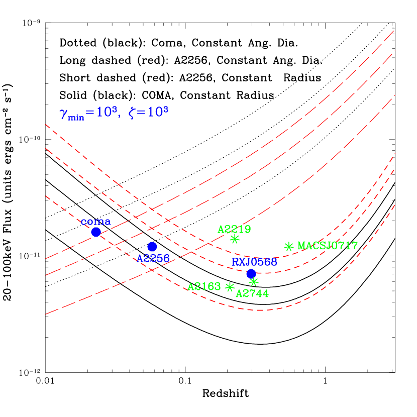
Figure 1: Predicted variations of the HXR flux with redshift assuming a constant metric (solid and dashed) or angular (dotted and long-dashed) diameters, using COMA (black and) and A2256 (red) parameters assuming $\zeta=\gamma_{\rm min}=10^{3}$. In each group the IC photon spectral index $\Gamma=2.25,2.0,1.75$, from top to bottom. Filled circles based on observations and stars based on the estimates given in Table 1.

3 OBSERVATIONS AND ANALYSIS

3.1 Description of Observations

Cluster 1E0657-56 was observed with RXTE during 95 separate pointings from 2002 August 19 to 2003 April 3, collecting approximately 400,000 seconds of data. After filtering the PCA data by following the standard selection criteria, we obtained a total of 309,630 seconds of good PCA data. During the campaign, only PCU 0 and PCU 2 were on. Since PCU 0 had lost its propane guard layer, in order to ensure that we have the best possible calibration, we used only the PCU 2 detector. The selection criteria involved excluding data obtained when the detector pointing was more than $0.02{{}^{\circ}}$ off the source, excluding data obtained when the Earth elevation angle was less than $10{{}^{\circ}}$, and excluding times near passage through the South Atlantic Anomaly which caused large variations in the count rate.

The amount of good time for each of the two HEXTE detector clusters is about one-third that for the PCA data: 105,450 seconds for Cluster A and 105,510 seconds for Cluster B. The ratio of HEXTE net time to PCA net time is reasonable, since each HEXTE cluster spent half of the time for background measurement and a fraction of the time was lost due to electronic dead time caused by cosmic rays.

The PCA background was estimated using the ftool pcabackest (v 3.0) with the “L7/240” model provided by the RXTE GOF (Guest Observer Facility). The estimator program used the model known as ${\tt pca\_bkgdcmfaint17\_eMv20051128.mdl}$ as the background model, which in turn took into consideration the instantaneous particle-induced intrinsic instrument background and activation - mainly due the SAA (South Atlantic Anomaly) passages - as well as the the cosmic X-ray background. We note here that the above background model, available from HEASARC at NASA’s GSFC (Dr. Craig Markwardt, priv. comm.) allows robust estimate of background up to $\sim 30$ keV even for faint sources such as 1ES0657-56.

We used the top layer of PCU 2 in the $3-30$ keV range. The mean background subtracted PCU2 count rate was $1.418\pm 0.007$ count s^-1 in the top layer over this band. For the response matrix, we used the standard PCA response matrix, generated via the ${\tt pcarsp}$ software tool (ver. 10.1), as appropriate to the beginning of the observations (2002 August); while the RXTE PCA response matrix changes with time, the change is gradual, and the values of spectral fits obtained using the matrix appropriate for the end of the observations (2003 April) showed no discernible difference. For HEXTE, the background subtracted count rates over the 20 $\sim$ 70 keV energy band were $0.0103\pm 0.0227$ count s^-1 and $0.0700\pm 0.0192$ count s^-1 for HEXTE detector clusters A and B, respectively; above 70 keV, the source was clearly not detected. We used the standard redistribution files, xh97mar20c_pwa_64b.rmf and xh97mar20c_pwb013_64b.rmf, with the standard HEXTE effective area files available through HEASARC.

While the RXTE data clearly detected the cluster, an inclusion of higher spectral resolution data allows a better constraint on the temperature of the thermal component and thus better constraints on the nature of the non-thermal emission. To this end, we considered the published ASCA data, but because the best statistical accuracy was provided in the XMM-Newton data, we extracted and analyzed archival spectra collected during the XMM-Newton pointing in 2000 October 20-21. We reduced the data using a procedure described in Andersson & Madejski (2004), but here, we used the ${\tt XMMSAS\_20050815}$ release of the XMM-Newton data analysis software. We screened the data against any obvious flares; this meant any segments of data with the total count rate greater than 12 counts s^-1 for pn, and 4.5 and counts s^-1 for either MOS. After cleaning, the effective exposure times are 24,916 s for the MOS1 data, 24813 s for the MOS2 data, and 21,704 s for the pn data. We note that the detailed analysis of the XMM-Newton data for this cluster - and in particular, the analysis of the spatial structure - will be presented in Andersson et al (in preparation). For all three XMM-Newton detectors, we extracted source counts from a region of $4^{\prime}$ radius around the centroid of the count distribution. For background, we used an annulus with inner and outer radii of $8^{\prime}$ and $12^{\prime}$, with all obvious point sources removed. We also removed the data corresponding to the Cu K line in the pn camera, corresponding to 7.9 to 8.2 keV spectral range. The data were grouped to include at least 40 counts per bin for the pn data files, and 25 counts per bin for the MOS data files. We used the standard instrument resolution matrices and effective area files as released in the SAS version as above. In the subsequent analysis, we restricted the two MOS and pn data to the 1 - 10 keV range, to avoid any residual cross-calibration problems between the three instruments.

3.2 Analysis and Spectral Fitting

3.2.1 RXTE Data

We first present an analysis of the RXTE observations and then a joint analysis of the RXTE and XMM-Newton data. In all subsequent fits we fix the redshift at 0.296. The models consist of a mekal thermal emission component, where we also allow a second component, either thermal, or a power law. We first use a single thermal mekal model to fit the RXTE data. The model includes a cold absorption due to neutral gas in the line of sight in our Galaxy. Since the RXTE data alone do not constraint the Galactic column density, we fix this parameter at $4.6\times 10^{20}$ cm^-2, the value from radio measurements, but also consistent with the best fit to ASCA data (Liang et al. 2000). We note that all errors quoted correspond to 90% confidence limits.

The best fit temperature under an assumption of a simple, one-temperature mekal model is $12.1\pm 0.4$ keV. This is in moderate agreement with the value $14.5_{-1.7}^{+2.0}$ keV determined from a joint fit to the ROSAT and ASCA data (Liang et al. 2000), and the value $14.8_{-1.2}^{+1.7}$ keV from Chandra (Markevitch et al. 2002). The metal abundance is $A=0.16\pm 0.04$ Solar, which is moderately lower than the value $A=0.33\pm 0.16$ from the joint ROSAT and ASCA data but is in good agreement with the Chandra value $0.11\pm 0.11.$ The best-fit model yields the $\chi^{2}$ of $114$ for $98$ degrees of freedom. The ratio of the RXTE data to the best-fit mekal model indicates systematic upward rise above 10 keV, suggesting that an extra component may be required. If we adopt this secondary component to be a power-law, then $\chi^{2}$ is $102$ (96 degrees of freedom), with poorly determined index ($\Gamma>2$). The 90% confidence interval of the power-law flux in the 20–100 keV range is $\left(0.3\pm 0.2\right)F_{0}$. We thus conclude that even from the RXTE data alone, we have a marginal but suggestive detection of hard X-ray flux in 1E06567-56.

3.2.2 XMM-Newton Data

The XMM-Newton data extracted as above were first fitted to a model including absorption due to neutral gas with Solar abundances and a thermal (mekal) plasma. Since the absolute calibration of the three XMM-Newton detectors might vary, we allowed the respective normalizations not to be tied to each other. The best fit absorption was close to the value inferred from the radio data of Liang et al. (2000), with the column $2.8\pm 1.0\times 10^{20}$ cm^-2, but here, inclusion of the MOS data below 1 keV altered the resulting best fit column to $5\pm 0.5\times 10^{20}$ cm^-2, We concluded that the column derived from the XMM-Newton data is consistent with $4.6\times 10^{20}$ cm^-2 cited by Liang et al. (2000), and used that value in all subsequent fits. The temperature of the mekal component was $12.0\pm 0.5$ keV, and elemental abundances $0.24\pm 0.04$ Solar, consistent with all data sets above. The fit is acceptable, at $\chi^{2}=1367$ for 1408 d.o.f.

Table 2 PARAMETERS FROM SPECTRAL FITTINGS

Data Set	Parameter	Single Thermal	Double-Thermal	Thermal+Power Law
	$\left(n_{H}/10^{20}{\Large\ {\rm cm}}^{-2}\right)$	$4.6^{f}$	–	$4.6^{f}$
	$kT_{1}$ $\left({\rm keV}\right)$	$12.1\pm 0.4$	–	$11.7\pm 0.5$
	$kT_{2}$ $\left({\rm keV}\right)$	–	–	–
RXTE	Abundance (Solar)	$0.16\pm$ $0.04$	–	$0.25\pm 0.08$
	Photon Index	–	–	$>2$
	${F_{20keV}^{100keV}}/F_{0}$	–	–	$0.3\pm 0.2$
	$\chi^{2}/dof$	$114/98$	–	$102/96$
	$\left(n_{H}/10^{20}{\Large\ cm}^{-2}\right)$	$2.8\pm 1.0$	$4.6^{f}$	$4.6^{f}$
	$kT_{1}$ $\left({\rm keV}\right)$	$12.1\pm 0.2$	$10.1\pm 0.9$	$11.2\pm 0.8$
RXTE and	$kT_{2}$ $\left({\rm keV}\right)$	–	$50\,(>30)$	–
XMM	Abundance (Solar)	$0.19\pm 0.03$	$0.19\pm 0.03$	$0.22\pm 0.04$
	Photon Index	–	–	$1.6\pm 0.2$
	$F_{20keV}^{100keV}/F_{0}$	–	$0.5\pm 0.3$	$0.5\pm 0.3$
	$\chi^{2}/dof$	$1483/1508$	$1471/1506$	$1464/1506$

$F_{0}=10^{-11}\,{\rm erg\,cm}^{-2}\,{\rm s}^{-1}$
^f denotes parameter fixed at the given value

3.2.3 Joint RXTE and XMM-Newton Data

In the analysis below, we include both the RXTE and XMM-Newton data, since the very good effective area of the instrument coupled with good spectral resolution of its detectors allows tighter constraints on spectral parameters for the emission detected below $\sim 10$ keV, and thus mainly on the thermal component. However, the only reliable approach here is to perform the spectral fitting simultaneously.

The joint analysis of the RXTE and XMM-Newton data provide more evidence of the need for a secondary component. We use the XMM-Newton and RXTE data over the bandpasses as above; we allow the normalization of the RXTE instruments to be different than that for the XMM-Newton instruments, which in turn are allowed to vary among themselves. A single isothermal (mekal) fit yields an adequate fit, with $\chi^{2}$ of 1483 for 1508 degrees of freedom. The hydrogen column density $n_{H}$ is $\left(2.8\pm 1.0\right)\times 10^{20}$ cm^-2, which is marginally lower than the Galactic value of Liang et al. (2000) (see the discussion above); in the subsequent fits we adopt the value of Liang et al. (2000) of $4.6\times 10^{20}$ cm^-2. Regardless of the exact value of absorption, the plasma temperature is $12.1\pm 0.2$ keV, and elemental abundances are $0.19\pm 0.03$ Solar. We note that the true errors on those quantities are only approximate, since as pointed out by Markevitch et al. (2002; 2004), this cluster shows some temperature structure, while we use an average temperature.

Adding a power-law component to the isothermal model improves the $\chi^{2}$ value, which is now 1464/1506 d.o.f. Such change in $\chi^{2}$ - with addition of two parameters - is very significant (at more than 99.9%). The temperature in this case decreases to $11.2\pm 0.8$ keV. The photon index is $1.6\pm 0.3$ and the non-thermal flux in the 20–100 keV energy band is $\left(0.5\pm 0.2\right)F_{0}.$ In the context of statistical significance of raw counting rates, at energies above 20 keV - where the power law model dominates - the excess (over the value predicted by the thermal model) corresponds to $\sim 0.8\sigma$ and $2.8\sigma$ for HEXTE Cluster A and B, respectively. For the purpose of illustration, we show the unfolded spectrum of the data fitted to a single-temperature thermal model in Figure 2, while Figure 3 shows the confidence levels of the two fit parameters, photon index vs. the flux of the non-thermal component, for our preferred two-component model.

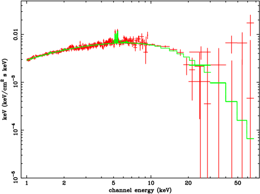
Figure 2: Unfolded spectrum of the cluster 1E0657-56, where the XMM-Newton and RXTE data were fitted with a single-temperature thermal (mekal) model, plotted here as the solid-line histogram. For the purpose of clarity of the plot, prior to plotting, the XMM-Newton data were scaled by a cross-normalization factor, close to unity, to agree with the RXTE data.

Alternatively, this secondary, hot component can be modeled via another thermal plasma spectral component. Using this parametrization (and assuming that only the temperature and normalization differ from the lower $T$ component), we inferred its temperature to be $50\,(>30)$ keV. The $20-100$ keV flux of this component is also $0.5\pm 0.2\times F_{0}$. Now the lower $T$ component has a temperature of $10.1\pm 0.9$ keV. While we cannot clearly exclude this interpretation on the quality-of-fit grounds ($\chi^{2}$ is 1471 for 1506 d.o.f.), we argue in Sec. 4 that the power law spectral shape provides for a more viable interpretation of the secondary component.

Figure 3: Confidence regions (corresponding to $\chi^{2}_{min}+2.3,4.6,$ and 9.2) on the best fit parameters for the spectral fits to the joint XMM-Newton , RXTE PCA, and HEXTE data for cluster 1E0657-56 for the photon index of the non-thermal X-ray component and its 20 - 100 keV flux (in units of $10^{-12}$ erg cm^-2 s^-1). See the text for details.

4 SUMMARY AND DISCUSSION

Radio observations of diffuse emission from ICM show presence of non-thermal activity in many clusters, especially in those with high SXR emitting gas temperatures (and luminosity) and showing recent merger activity. A list of such clusters is shown in Table 1. Detections of HXR emission exceeding the levels expected from the thermal gas have been reported by two groups using different instruments. This enables a quantitative investigation of the nature and origin of the non-thermal activity. The radio observations alone indicate presence of extreme relativistic electrons ($\gamma\sim 10^{4}$). Assuming equipartition between the relativistic electrons and the magnetic field we estimate a volume-averaged magnetic field value in the range of 0.5 to 2 $\mu{\rm G}$ (see Table 1), in rough agreement with (line-of-sight averaged) field strengths deduced from Faraday rotation measurements. In the case of Coma the magnetic field deduced from Faraday rotation of $2-3\,\mu{\rm G}$, implies conditions far from equipartition if we assume a homogeneous source; the field energy density is about 25 times larger than that of the electrons. This discrepancy can be resolved by an inhomogeneous model; e.g. the two phase model proposed by Brunetti et al. (2001) that implies a magnetic field profile, or if there was 25 times more energy in nonthermal protons than electrons.

If the HXR radiation is due to IC scattering of CMB photons by the the same electrons that produce the synchrotron radio emission, which we have argued to be the simplest scenario, such high magnetic files would imply IC fluxes in the $20-100$ keV range of about $10^{-2}F_{0}$ while both Coma and A2256 show fluxes higher than $F_{0}$. Production of HXRs at this level require magnetic fields of about $0.1\,\mu{\rm G}$ (or partition parameter $\zeta\sim 10^{3}$) which raises the required energy of the non-thermal electrons (${\cal E}_{e}\propto\zeta^{1/2}$). For example for Coma and A2256 the observed HXR fluxes require ${\cal E}_{e}=2\times 10^{-13}$ and $1.5\times 10^{-12}$ erg ${\rm cm}^{-3}$, respectively, which are comparable to the energy density of the CMB ($4.6\times 10^{-13}$ erg ${\rm cm}^{-3}$). Assuming similar conditions for other clusters, several years ago we identified 1E0657-56 and A2219 as possible candidate for having detectable HXR fluxes. Here, we have described these observations of 1E0657-56 and the results of our spectral fitting to these data alone and to the RXTE data combined with the SXR data from XMM-Newton. In the future, attempts should be made to observe other clusters in Table 1, and any newly discovered cluster with a relatively high temperature and redshift, an ample sign of substructure and/or mergers, and, of course, with a strong diffuse radio emission. A low value of magnetic field indicated by Faraday rotation measurements or estimated via equipartition argument will also be good justification for HXR observations.

We have shown that a thermal component plus a non-thermal tail described as a power law with spectral index $\Gamma=1.6$ containing $\sim 0.5F_{0}$ of the $20-100$ keV flux provides an acceptable fit. This flux is fortuitously close to the value of $0.52\,F_{0}$ we estimate by scaling the Coma and A2256 observations. (Note that the equipartition (i.e. $\zeta=1$) magnetic field and flux for this cluster would be $\sim 1\,\mu{\rm G}$ and $0.02\,F_{0}$.) This agreement is somewhat encouraging so that we believe that the chances are even better for detection of HXR emission from Abell 2219, a good candidate at a moderate redshift, and a recently discovered cluster, MACJ7017, with even higher $z$ than 1E0657-56. As is the case for Coma and Abell 2256, these clusters also require high nonthermal electron energy densities; ${\cal E}_{e}=[1.0,1.8,8.5]\times 10^{-13}$ erg ${\rm cm}^{-3}$ for Abell 2219, 1E0657-56 and MACSJ0717, respectively. These are even closer to the CMB densities at their respectively higher redshifts. In general the required electron energies are about 1 to 10 % of the energy density of the thermal gas of few times $10^{-11}$ erg ${\rm cm}^{-3}$ which is also comparable to the gravitational potential energy density of the cluster. This means a very efficient acceleration process.

Regarding the spectral fits to 1E0657-56, as shown in Table 2, we also obtain an acceptable fit with a double temperature thermal model with a second component with $kT=50$ keV and a normalization implying a volume emission measure ($EM$) for this component which is a significant fraction ($\sim 10\%$) of that of the lower temperature component. Indeed Markevitch (2005) finds evidence for such a high $T$ component behind the shock near the bullet based on the recent Chandra Observatory data. However, this has a much smaller $EM$ than is required for fitting the data with a two temperature model. In fact a high $T$ component with such a large $EM$ would have been easily detected by Markevitch (2005). Clearly more and deeper observations of the clusters in Table 1 can clarify this situation considerably. In particular, deep observations with imaging HXR instruments – such as those with the proposed NuSTAR satellite – which can provide information about the spatial distribution of the HXRs would be very valuable.

In spite of the uncertainties about the exact character of the observed radiation spectra and the emission mechanism, and in spite of the meagerness of the data, the acceleration mechanism of electrons can be constrained significantly. The lifetimes of electrons with energies in the range $200\,{\rm keV}\leq E\leq 200\,{\rm GeV}$ are longer than the crossing time, $T_{\rm cross}\sim 3\times 10^{6}$ yr. Therefore, these electrons will escape the cluster and radiate most of their energy outside of the cluster unless there exists some scattering agent with a mean free path $\lambda_{\rm scat}\sim 1$ kpc to trap the electrons in the ICM for at least a timescale of $T_{\rm esc}=(R/\lambda_{\rm scat})T_{\rm cross}\sim 3\times 10^{9}$ yr, for cluster size $R\sim 1$Mpc. Turbulence can be this agent and can play a role in stochastic acceleration directly, or indirectly in acceleration by shocks, presumably arising from merger events. Several lines of argument point to an ICM which is highly turbulent, and there has been considerable discussion of these aspects of the problem in the recent literature (see, e.g., Cassano & Brunetti 2005). These aspect are explored in P01, but the upshot of which is that we require injection of high energy electrons, presumably from galaxies and AGNs, and that the acceleration process is episodic on time scale of $\sim 10^{8}$ to $10^{9}$ yr. Whether the electrons are injected directly by past and current AGN activity, or are produced by the interaction with the thermal gas of cosmic ray protons escaping the galaxies would be difficult to determine now. There are however constrains on both these scenarios (see e.g. Blasi 2003).

References

- (1) Allen, S. A., & Fabian, A. C. 1998, MNRAS, 297, 57
- (2) Andersson, K., & Madejski, G., 2004, ApJ, 607, 190
- (3) Blasi, P. 2000, ApJ, 532, L9
- (4) Blasi, P. 2003, in “Matter and Energy in Clusters of Galaxies,” ASP Conf. Series 301, eds. S. Bowyer & C.-Y. Hwang, 203 (astro-ph/0207361)
- (5) Bowyer, S. 2003, in “Matter and Energy in Clusters of Galaxies,” ASP Conf. Series 301, eds. S. Bowyer & C-Y Hwang, 125
- (6) Brunetti, G., Setti, G., Feretti, L., & Giovannini, G. 2001, MNRAS, 320, 365
- (7) Buote, D. A. 2001, ApJ, 553, L15
- (8) Carilli, C., & Taylor, G. B. 2002, ARAA, 40, 319
- (9) Cassano, R., & Brunetti, G. 2005, MNRAS, 357, 1313
- (10) Clarke, T. E. et al. 2001, ApJ, 547, L111
- (11) Clarke, T. E. 2003 in “Matter and Energy in Clusters of Galaxies,” ASP Conf. Series 301, eds. S. Bowyer & C.-Y. Hwang, 185
- (12) Enßlin, T. A., Lieu, R., & Biermann, P. 1999, A&A, 344, 409
- (13) Feretti, L., Brunetti, G., Giovannini, G., Govoni, F., & Setti, G. 2000, in “Constructing the Universe with Clusters of Galaxies,” Proc. IAP 2000 meeting, Paris, France, eds. F. Durret & D. Gerbal (astro-ph/0009346)
- (14) Feretti, L., Fusco-Femiano, R., Giovannini, G., & Govoni, F. 2001, A&A, 373, 106
- (15) Fusco-Femiano, R., et al. 1999, ApJ, 513, L21
- (16) Fusco-Femiano, R., et al. 2000, ApJ, 534, L7
- (17) Fusco-Femiano, R., et al. 2003, A&A, 398, 441
- (18) Fusco-Femiano, R., et al. 2004, ApJ, 602, 73
- (19) Fusco-Femiano, R., Landi, R., & Orlandini, M. 2005, ApJ, 624, L69
- (20) Giovannini, G., & Feretti, L. 2000, NewA, 5, 535
- (21) Giovannini, G., Tordi, M., & Feretti, L. 1999, NewA, 4, 141
- (22) Giovannini, G., Feretti, L., Venturi, T., Kim, K.-T., & Kronberg, P. 1993, ApJ, 406, 399
- (23) Govoni, F., et al. 2003 in “Matter and Energy in Clusters of Galaxies,” ASP Conf. Series 301, eds. S. Bowyer & C.-Y. Hwang, 501
- (24) Govoni, F., & Feretti, L. 2004, Int. J. Mod. Phys. D13, 1549 (astro-ph/0410182)
- (25) Gruber, D., & Rephaeli, Y. 2002, ApJ, 565, 877
- (26) Hudson, D. S., Henriksen, M. J., & Colafrancesco, S. 2003, ApJ, 583, 706
- (27) Kim, K.-T., et al. 1990, ApJ, 355, 29
- (28) Liang, H., Hunstead, R. W., Birkinshaw, M., & Andreani, P. 2000, ApJ, 544, 686
- (29) Lieu, R. et al. 1996, Science, 274, 1335
- (30) Markevitch, M., et al, 2002, ApJ, 567, L27
- (31) Markevitch, M., et al, 2004, ApJ, 606, 819
- (32) Markevitch, M. 2005, in “The X-ray Universe 2005,” (astro-ph/0511345)
- (33) Petrosian, V. 1973, ApJ, 186, 291
- (34) Petrosian, V. 2001, ApJ, 557, 560
- (35) Rephaeli, Y. 1979, ApJ, 227, 364
- (36) Rephaeli, Y. et al. 1999, ApJ, 511, L21
- (37) Rephaeli, Y., & Gruber, D. 2002, ApJ, 579, 587
- (38) Rephaeli, Y., & Gruber, D. 2003, ApJ, 595, 137
- (39) Rephaeli, Y., Gruber, D., & Arieli, Y. 2006, ApJ, in press (astro-ph/0606097)
- (40) Rosetti, M., & Molendi, S. 2004, A&A, 414, L41
- (41) Rudnick, L., & Blundell, K. M. 2003, ApJ, 588, 143
- (42) Rybicki, G., & Lightman, A. 1979, “Radiative processes in Astrophysics,” Wiley-Interscience
- (43) Schlickeiser, R., Sievers, A., & Thiemann, H. 1987, A&A, 182, 21
- (44) Schuecker, P., et al. 2001, A&A, 378, 408
- (45) Thierbach, M., Klein, U., & Wielebinski, R. 2003, A&A, 397, 53