Scalar-field-dominated cosmology with a transient accelerating phase

Abstract

A new cosmological scenario driven by a slow rolling homogeneous scalar field whose exponential potential $V(\Phi)$ has a quadratic dependence on the field $\Phi$ in addition to the standard linear term is discussed. The derived equation of state for the field predicts a transient accelerating phase, in which the Universe was decelerated in the past, began to accelerate at redshift $z\sim 1$, is currently accelerated, but, finally, will return to a decelerating phase in the future. This overall dynamic behavior is profoundly different from the standard $\Lambda$CDM evolution, and may alliviate some conflicts in reconciling the idea of a dark energy-dominated universe with observables in String/M-theory. The theoretical predictions for the present transient scalar field plus dark matter dominated stage are confronted with cosmological observations in order to test the viability of the scenario.

Introduction.—The idea of a dark energy-dominated universe is a direct consequence of a convergence of independent observational results, and constitutes one of the greatest challenges for our current understanding of fundamental physics review . Among a number of possibilities to describe this dark energy component, the simplest and most theoretically appealing way is by means of a cosmological constant $\Lambda$, which acts on the Einstein field equations as an isotropic and homogeneous source with a constant equation of state (EoS) $w\equiv p/\rho=-1$. Although cosmological scenarios with a $\Lambda$ term may explain most of the current astronomical observations, from the theoretical viewpoint it is really difficult to reconcile the small value required by observations ($\simeq 10^{-10}\rm{erg/cm^{3}}$) with estimates from quantum field theories ranging from 50-120 orders of magnitude larger weinberg , which makes a complete cancellation (from some unknown string theory symmetry) seem also plausible.

However, if the cosmological term is null or it is not decaying in the course of the expansion decaying , something else must be causing the Universe to speed up. The next simplest approach toward constructing a model for an accelerating universe is to work with the idea that the unknown, unclumped dark energy component is due exclusively to a minimally coupled scalar field $\Phi$ (quintessence field) which has not yet reached its ground state and whose current dynamics is basically determined by its potential energy $V(\Phi)$. This idea has received much attention over the past few years and a considerable effort has been made in understanding the role of quintessence fields on the dynamics of the Universe quintessence . Examples of quintessence potentials are ordinary exponential functions $V(\Phi)=V_{0}\exp{(-\lambda\Phi)}$ RatraPeebles ; fj ; wetterich , simple power-laws of the type $V(\Phi)=V_{0}\Phi^{-n}$ power_law , combinations of exponential and sine-type functions $V(\Phi)=V_{0}\exp{(-\lambda\Phi)}[1+A\sin{(-\nu\Phi)}]$ dodelson , among others (see, e.g., review and references therein). In particular, the exponential example above, originally investigated in Ref. RatraPeebles , constitutes a kind of benchmark of quintessence scenarios and has been largely explored in the literature, both in its theoretical and observational aspects fj . As shown in Ref. wetterich this particular class of potentials also leads to an attractor-type solution with $\Omega_{\Phi}=\rho_{\Phi}/(\rho_{\Phi}+\rho_{i})=n/\lambda^{2}$, where $\Omega_{\Phi}$ and $\rho_{i}$ are, respectively, the scalar field density parameter and the energy density of the other component scaling as $a^{-n}$. All these quintessence scenarios are based on the premise that fundamental physics provides motivation for light scalar fields in nature so that a quintessence field $\Phi$ may not only be identified as the dark component dominating the current cosmic evolution but also as a bridge between an underlying theory and the observable structure of the Universe.

If, however, it is desirable (and we believe so) a more complete connection between the physical mechanism behind dark energy and a fundamental theory of nature, one must bear in mind that an eternally accelerating universe, a rather generic feature of quintessence scenarios, seems not to be in agreement with String/M-theory predictions, since it is endowed with a cosmological event horizon which prevents the construction of a conventional S-matrix describing particle interactions fischler . Although the transition from an initially decelerated to a late-time accelerating expansion is becoming observationally established ms , the duration of the accelerating phase, depends crucially on the cosmological scenario and, several models, which includes our current standard $\Lambda$CDM scenario, imply an eternal acceleration or even an accelerating expansion until the onset of a cosmic singularity (e.g., the so-called phantom cosmologies ph ). This dark energy/String theory conflict, therefore, leaves us with the formidable task of either finding alternatives to the conventional S-matrix (or, equivalently, defining observables in a string theory described by a finite dimensional Hilbert space) or constructing a quintessence model of the Universe that predicts the possibility of a transient acceleration phenomenon.

In this Letter, we follow the latter route and investigate a new quintessence scenario driven by a rolling homogeneous scalar field whose exponential potential $V(\Phi)$ predicts a transient accelerating phase followed by an eternally decelerated universe. The potential, which has a quadratic dependence on the field $\Phi$ in addition to the standard linear term, is obtained through a simple ansatz and fully reproduces the exponential potential studied by Ratra and Peebles in Ref. RatraPeebles in the limit of the dimensionless parameter $\alpha\rightarrow 0$. For all values of $\alpha\neq 0$, however, the potential is dominated by the quadratic contribution present in the exponential function, admiting a wider range of solutions. We also derive analytically all the main background equations of the model to show that a transient accelerating phase is a feature of this class of potentials, which in turn may reconcile the observed acceleration of the Universe with the requirements of String/M theories. The observational viability of our model is also tested by confronting its predictions with the most recent SNe Ia and Cosmic Microwave Background (CMB) data.

The Model.—Let us first consider a homogeneous, isotropic, spatially flat cosmologies described by the Friedmann-Robertson-Walker (FRW) flat line element, $ds^{2}=-dt^{2}+a^{2}(t)(dx^{2}+dy^{2}+dz^{2}),$ where $a(t)$ is the cosmological scalar factor and we have set the speed of light $c=1$. The action for the model is given by $S={m^{2}_{pl}/16\pi}\int d^{4}x\sqrt{-g}[R-{1\over 2}\partial^{\mu}\Phi\partial_{\mu}\Phi-V(\Phi)+{\cal{L}}_{m}]$, where $R$ is the Ricci scalar and $m_{pl}\equiv G^{-1/2}$ is the Planck mass. The scalar field is assumed to be homogeneous, such that $\Phi=\Phi(t)$ and the Lagrangian density ${\cal{L}}_{m}$ includes all matter and radiation fields.

1. A scalar-field-dominated universe.

For now, it will be assumed that the cosmological fluid is composed only of a quintessence field $\Phi$ (${\cal{L}}_{m}=0$), whose energy-momentum tensor reads $T^{\mu\nu}_{\Phi}=\partial^{\mu}\Phi\partial^{\nu}\Phi-{1\over 2}g^{\mu\nu}\left[\partial^{\alpha}\Phi\partial_{\alpha}\Phi+2V(\Phi)\right]\;$. The conservation equation for this $\Phi$ component takes the form

$$\dot{\rho}_{\Phi}+3H(\rho_{\Phi}+p_{\Phi})=0\;,$$ (1)

or, equivalently, $\ddot{\Phi}+3H\dot{\Phi}+V^{\prime}(\Phi)=0$, where $\rho_{\Phi}={1\over 2}\dot{\Phi}^{2}+V(\Phi)$ and $p_{\Phi}={1\over 2}\dot{\Phi}^{2}-V(\Phi)$ are, respectively, the scalar field energy density and pressure, and dots and primes denote, respectively, derivatives with respect to time and to the field. By integrating the above equation, we also obtain the following relation for the scalar field $\Phi$, i.e.,

$$\frac{\partial\Phi}{\partial a}=\sqrt{-\frac{m_{\rm pl}^{2}}{8\pi a}\frac{1}{\rho_{\Phi}}\frac{\partial\rho_{\Phi}}{\partial a}}\;,$$ (2)

where $H\equiv\dot{a}/a$ stands for the Hubble parameter, and the Friedmann equation $H^{2}={8\pi}\rho_{\Phi}/3m^{2}_{\rm pl}$ has been explicitly used.

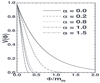
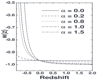
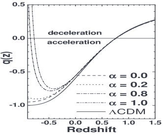
Figure 1: Some of the physical quantities discussed in the text. a) The potential $V(\Phi)$ as a function of the field [Eq. (6)] for some selected values of the parameter $\alpha$. b) The plane $w(z)-z$. Note that $w(z)$ reduces to a constant EoS $w\simeq-0.96$ [$\lambda={\cal{O}}(10^{-1})$] in the limit $\alpha\rightarrow 0$ while $\forall$ $\alpha\neq 0$ it was $-1$ in the past and $\rightarrow+1$ in the future. c) The deceleration parameter as a function of the redshift for selected values of $\alpha$ and $\Omega_{m,0}=0.27$. For values of $\alpha\neq 0$ the cosmic acceleration is a transient phenomenon. In particular, for $\alpha=1.0$ the transition redshifts happen at $z_{a/d}\simeq\pm 0.77$. The $\Lambda$CDM case (solid line) is also shown here for the sake of comparison.

In order to proceed further, let us adopt the following ansatz on the scale factor derivative of the energy density

$$\frac{1}{\rho_{\Phi}}\frac{\partial\rho_{\Phi}}{\partial a}=-\frac{\lambda}{a^{1-2\alpha}}\;,$$ (3)

where $\alpha$ and $\lambda$ are positive parameters while the factor 2 was introduced for mathematical convenience. From a direct combination of Eqs. (2) and (3), the following expression for the scalar field is obtained

$$\Phi(a)-\Phi_{0}=\frac{1}{\sqrt{\sigma}}\ln_{1-\alpha}(a)\;,$$ (4)

where $\Phi_{0}$ is the current value of the field $\Phi$ (from now on the subscript 0 denotes present-day quantities), $\sigma={8\pi/\lambda m_{\rm pl}^{2}}$ and the generalized function $\ln_{1-\xi}$, defined as $\ln_{1-\xi}(x)\equiv{(x^{\xi}-1)/\xi}$, reduces to the ordinary logarithmic function in the limit $\xi\rightarrow 0$ abramowitz . To derive the potential $V(\Phi)$ for the above scenario, we first note, from the definitions of $\rho_{\Phi}$ and $p_{\Phi}$ [see Eqs. (7) and (9) below], that the potential $V(a)$ is given by

$$V(a)=\left[1-{\lambda\over 6}a^{2\alpha}\right]\rho_{\Phi,0}\exp\left[-{\lambda\over 2}\ln_{1-\alpha}(a^{2})\right].$$ (5)

By inverting Eq. (4) and inserting $a(\Phi)$ into the above expression, the potential $V(\Phi)$ is readily obtained

$$V(\Phi)=f(\alpha;\Phi)\rho_{\Phi,0}\exp\left[-\lambda\sqrt{\sigma}\left(\Phi+{\alpha\sqrt{\sigma}\over 2}\Phi^{2}\right)\right]\;,$$ (6)

where $f(\alpha;\Phi)=[1-{\lambda\over 6}(1+\alpha\sqrt{\sigma}\Phi)^{2}]$. The important aspect to be emphasized at this point is that in the limit $\alpha\rightarrow 0$ Eqs. (4) and (6) fully reproduce the exponential potential studied by Ratra and Peebles in Ref. RatraPeebles , while $\forall$ $\alpha\neq 0$ the scenario described above represents a generalized model which admits a wider range of solutions. In order to exemplify this more general behavior, Fig. (1a) shows the potential $V(\Phi)$ for some selected values of the parameter $\alpha$ and the fixed value of $\lambda=10^{-1}$.

2. Scalar field + dark matter model.

In what follows, it will be assumed that the cosmological fluid is composed of non-relativistic matter (dark plus baryonic) and the quintessence field $\Phi$. The Friedmann equation derived from the action above now reads $H^{2}={8\pi/3m^{2}_{\rm pl}}\rho$, where $\rho=\rho_{\Phi}+\rho_{m}$ is the total energy density.

A direct integration of Eq. (3) gives the scalar field energy density as a function of the scale factor, i.e.,

$$\rho_{\Phi}(a)=\rho_{\Phi,0}\exp\left[-{\lambda\over 2}\ln_{1-\alpha}(a^{2})\right]\;.$$ (7)

Note that in the limit $\alpha\rightarrow 0$ the quintessence energy density (7) reduces to an usual power-law, $\rho_{\Phi}(a)\propto a^{-{\lambda}}$ (as predicted by ordinary exponential potentials RatraPeebles ), which clearly shows that this latter class of $V(\Phi)$ provides only a particular solution out a set of possible solutions that can be explored from a more general exponential law [see Eq. (6)]. Note also that now the term $1/\rho_{\Phi}$ in the square root of Eq. (2) must be replaced by $1/\rho$, so that by combining our ansatz (3) with the new Eq. (2), we find

$$\Phi-\Phi_{0}=\frac{1}{\sqrt{\sigma}}\int_{1}^{a}{\frac{a^{\prime\alpha-1}}{{\cal{F}}(a^{\prime})}}da^{\prime}\>,$$ (8)

where ${\cal{F}}(a)=\sqrt{(1+\Omega_{m}/\Omega_{\Phi})}$, with $\Omega_{m}$ and $\Omega_{\Phi}$ representing the matter and quintessence density parameters, respectively. As one may easily check, the above expression for $\Phi(a)$ reduces to Eq. (4) for $\Omega_{m}=0$. When combined numerically with Eq. (5), it also provides the potential $V(\Phi)$ for this realistic dark matter/energy scenario, which belongs to the same class of potentials as given in Eq. (6) and shown in Figure (1a).

Equation of state.—Without loss of generality to the subsequent analyses, from now on we particularize our study to the case $\lambda\simeq{\cal{O}}(10^{-1})$. Thus, by combining Eqs. (1) and (7), we also obtain the EoS for this quintessence component, i.e.,

$$w(a)=-1+{1\over 30}a^{2\alpha}\;,$$ (9)

which is shown as a function of the redshift parameter ($z=a^{-1}-1$) in Fig. (1b) for some selected values of the index $\alpha$. Differently from the ordinary exponential cases studied in Ref. RatraPeebles , the above EoS is a time-dependent quantity ($\forall$ ${\cal{\alpha}}\neq 0$) and reduces to a constant EoS $w=-1+{1\over 30}$ [$\simeq-0.96$] only in the limit $\alpha\rightarrow 0$, in agreement with our ansatz (3) and the energy density derived in Eq. (7). Note also that the EoS above (which must lie in the interval $-1\leq w(a)\leq 1$) is an increasingly function of time, being $\simeq-1$ in the past, $\simeq-0.96$ today, and becoming more positive in the future ($0$ at $a=30^{1/2\alpha}$ and $1/3$ at $a=40^{1/2\alpha}$). This amounts to saying that although the Universe will be eternally dominated by the quintessence field $\Phi$, it may not accelerate forever since the field will behave more and more as an attractive matter field. Some physical consequences of this unusual behavior are discussed as follows.

Transient Acceleration.— For a large interval of values for the parameter $\alpha$ the behavior of the EoS (9) leads to a transient acceleration phase and, as a consequence, may alleviate the dark energy/String theory conflict discussed earlier. To study this phenomenon, let us first consider the deceleration parameter, defined as $q=-a\ddot{a}/\dot{a}^{2}$ and shown in Figure (1c) as a function of the redshift parameter for some values of the index $\alpha$ and $\Omega_{m,0}=0.27$. As can be seen from this figure, $\forall$ $\alpha\neq 0$ the Universe was decelerated in the past, began to accelerate at $z_{*}\lesssim 1$, is currently accelerated but will eventually decelerate in the future. As expected from Eq. (9), this latter transition is becoming more and more delayed as $\alpha\rightarrow 0$. In particular, at $a=20^{1/2\alpha}$, $w(a)$ crosses the value $-1/3$, which roughly means the beginning of the future decelerating phase. A cosmological behavior like the one described above seems to be in agreement with the requirements of String/M-theory (as discussed in Refs. fischler ), in that the current accelerating phase is a transitory phenomenon (Another interesting example of transient acceleration is provided by the brane-world scenarios discussed in Ref. ss (See also js ).). As one may also check, the cosmological event horizon, i.e., the integral $\int{da/a^{2}H(a)}$ diverges for this transient scalar-field-dominated universe, thereby allowing the construction of a conventional S-matrix describing particle interactions within the String/M-theory frameworks. A typical example of an eternally accelerating universe, i.e., the $\Lambda$CDM model, is also shown in Fig. (1c) for the sake of comparison.

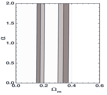
Figure 2: 68.3%, 95.4% and 99.73% c.l. in the plane $\Omega_{m,0}$ - $\alpha$ arising from SNe Ia and CMB data. Note that while the matter density parameter is well restricted to the interval $\Omega_{m,0}=0.25^{+0.06}_{-0.07}$ (at 95.4% c.l.), the current observational data cannot place restrictive bounds on the parameter $\alpha$.

Observational Constraints.—We study now some observational bounds on the cosmological scenario proposed above. We use to this end complementary data from the Supernova Legacy Survey (SNLS) collaboration (corresponding to the first year results of its planned five years survey) snls and the shift parameter from WMAP, CBI and ACBAR, defined as $R\equiv\Omega_{m}^{1/2}\int_{0}^{z}{dz^{\prime}/E(z^{\prime})}=1.716\pm 0.062$, where $z=1089$ is the redshift of recombination wmap . The SNLS sample used here includes 71 high-$z$ SNe Ia in the redshift range $0.2\lesssim z\lesssim 1$ and 44 low-$z$ SNe Ia compiled from the literature but analyzed in the same manner as the high-$z$ sample. This data-set is arguably (due to multi-band, rolling search technique and careful calibration) the best high-$z$ SNe Ia compilation to date, as indicated by the very tight scatter around the best fit in the Hubble diagram (we refer the reader to Ref. sne for details on statistical analyses involving SNe Ia and CMB data). Figure 2 shows the 68.3%, 95.4% and 99.73% confidence limits (c.l.) in the parametric space $\Omega_{m,0}$ - $\alpha$. Similarly to what happens with most of the time-dependent EoS parametrizations (see, e.g., sne ), the current observational bounds on the index $\alpha$ are considerably weak since it appears only in the exponential term of the energy density (7). We believe that the next generation of dark energy experiments dedicated to this issue (mainly those measuring the expansion history from high-$z$ SNe Ia, baryon oscillations, and weak gravitational lensing distortion by foreground galaxies – see, e.g., jedi ) will probe cosmology with sufficient accuracy to decide if values of $\alpha\neq 0$ are preferable from both theoretical and observational viewpoints (see also caldprl and references therein for more on this issue). For the combination of current SNe Ia and CMB data, the best-fit model occurs for values of $\Omega_{m,0}=0.25$ (${}^{+0.06}_{-0.07}$ at 95.4% c.l.) and $\alpha\simeq 1$ (with reduced $\chi_{\nu}^{2}\simeq 1.01$), which corresponds to a 9.8$h^{-1}$-Gyr-old, accelerating universe with a deceleration parameter $q_{0}=-0.58$ and transition redshifts $z_{a}=0.8$ (acceleration) and $z_{d}=-0.77$ (deceleration). A more detailed analysis of the cosmological model discussed here, as well as its conections with the inflationary scenario, will appear in a forthcoming communication.

Conclusions.—We have constructed a model wherein the quintessence field contributes as subdominant cosmological constant at the earlier stages of the universe so that the nucleossynthesis constraints are naturally satisfied. However, although subdominant for a long period (radiation and matter eras), the energy density of the field $\Phi$ is increasing in the course of expansion, and, finally, for a redshift of the order of a few, a quintessence dominated phase begins. As we have discussed [see Eq. (9)], a basic difference with other quintessence models is that the accelerating phase in the present scenario does not last forever. After some eons, the equation of state parameter describing the field component becomes more and more positive with the Universe, inevitably, returning to an expanding decelerating stage. Finally, we emphasize that the model makes definite predictions and is in agreement with the observational tests analyzed here.

This work is supported by CNPq - Brazil. JSA is also supported by FAPERJ No. E-26/171.251/2004.

References

- (1) P.J.E. Peebles and B. Ratra Rev. Mod. Phys. 75, 559 (2003); T. Padmanabhan, Phys. Rept. 380, 235 (2003); E. J. Copeland, M. Sami and S. Tsujikawa, hep-th/0603057.
- (2) S. Weinberg, Rev. Mod. Phys. 61, 1 (1989).
- (3) M. zer and M.O. Taha, Phys. Lett. B 171, 363 (1986); K. Freese et al., Nucl. Phys. B287, 797 (1987); J.C. Carvalho et al. J. A. S. Lima and I. Waga, Phys. Rev. D46, 2404 (1992); J.A.S. Lima and M. Trodden, Phys. Rev. D53, 4280 (1996).
- (4) R.R. Caldwell, R. Dave, P.J. Steinhardt, Phys. Rev. Lett. 80, 1582 (1998); S.M. Carroll, Phys. Rev. Lett., 81, 3067 (1998); K.R.S. Balaji and R.H. Brandenberger, Phys. Rev. Lett. 94, 031301 (2005).
- (5) B. Ratra and P.J.E. Peebles, Phys. Rev D37, 3406 (1988).
- (6) P.G. Ferreira and M. Joyce, Phys. Rev. D58, 023503(1998); A. Albrecht and C. Skordis, Phys. Rev. Lett. 84, 2076 (2000)
- (7) C. Wetterich, Astron. & Astrophys. 301, 321 (1995).
- (8) P.J.E. Peebles and B. Ratra, Astrophys. J. Lett. 325, L17 (1988); I. Zlatev, L-M. Wang , P.J. Steinhardt, Phys. Rev. Lett. 82, 896 (1999).
- (9) S. Dodelson et al., M. Kaplinghat and E. Stewart, Phys. Rev. Lett. 85, 5276 (2000)
- (10) W. Fischler, A. Kashani-Poor, R. McNees, and S. Paban, JHEP 3, 0107 (2001); S. Hellerman, N. Kaloper and L. Susskind, JHEP 3, 0106, (2001); J.M. Cline, JHEP 0108, 35 (2001); E. Halyo, JHEP 0110, 025 (2001).
- (11) M. S. Turner and A. G. Riess, Astrophys. J. 569, 18 (2002).
- (12) R.R. Caldwell, Phys. Lett. B545, 23 (2002).
- (13) M. Abramowitz and I. Stegun, Handbook of Mathematical Functions, Dover, New York, (1965). See also J.A.S. Lima, R. Silva and A.R. Plastino, Phys. Rev. Lett., 86, 2938 (2001).
- (14) V. Sahni and Y. Shtanov, JCAP 0311, 014 (2003).
- (15) J.S. Alcaniz and H. Stefancic, astro-ph/0512622.
- (16) P. Astier et al., Astron. Astrophys. 447, 31 (2006).
- (17) D.N. Spergel et al., Astrophys. J. Suppl. 148, 175 (2003).
- (18) T. Padmanabhan and T. R. Choudhury, MNRAS 344, 823 (2003); Y. Wang and M. Tegmark, Phys. Rev. Lett., 92, 241302 (2004). M. A. Dantas et al., astro-ph/0607060.
- (19) A Crotts et al., astro-ph/0507043. (see also http://jedi.nhn.ou.edu/).
- (20) R.R. Caldwell and E. V. Linder, Phys. Rev. Lett. 95, 141301 (2005).