The intracluster magnetic field power spectrum in Abell 2255

Abstract

Aims. The goal of this work is to constrain the strength and structure of the magnetic field in the nearby cluster of galaxies A2255. At radio wavelengths A2255 is characterized by the presence of a polarized radio halo at the cluster center, a relic source at the cluster periphery, and several embedded radio galaxies. The polarized radio emission from all these sources is modified by Faraday rotation as it traverses the magnetized intra-cluster medium. The distribution of Faraday rotation can be used to probe the magnetic field strength and topology in the cluster.

Methods. For this purpose, we performed Very Large Array observations at 3.6 and 6 cm of four polarized radio galaxies embedded in A2255, obtaining detailed rotation measure images for three of them. We analyzed these data together with the very deep radio halo image recently obtained by us. We simulated random 3-dimensional magnetic field models characterized by different power spectra and produced synthetic rotation measure and radio halo images. By comparing the simulations with the data we are able to determine the strength and the power spectrum of the intra-cluster magnetic field fluctuations which best reproduce the observations.

Results. The data require a steepening of the power spectrum spectral index from $n=2$, at the cluster center, up to $n=4$, at the cluster periphery and the presence of filamentary structures on large scales. The average magnetic field strength at the cluster center is 2.5 $\mu G$. The field strength declines from the cluster center outward with an average magnetic field strength calculated over 1 Mpc³ of $\sim$1.2 $\mu$G.

1 Introduction

The existence of magnetic fields associated with the intracluster medium in clusters of galaxies is now well established through different methods of analysis (see e.g. the review by Govoni & Feretti 2004, and references therein). The strongest evidence for the presence of cluster magnetic fields comes from radio observations. Magnetic fields are revealed through the synchrotron emission of cluster-wide diffuse sources, and from studies of the rotation measure (RM) of polarized radio galaxies. Other techniques, not discussed in this paper, include the study of inverse Compton hard X-ray emission (e.g. Fusco-Femiano et al. 2004, Rephaeli et al. 2006), cold fronts (e.g. Vikhlinin & Markevitch 2002) and magneto hydrodynamic simulations (e.g. Dolag et al. 2002).

Direct evidence for the presence of relativistic electrons and magnetic fields in clusters of galaxies comes from the detection, in an ever increasing number of galaxy clusters, of large-scale, diffuse, steep-spectrum synchrotron sources known as ’radio halos’ or ’relics’ depending on their morphology and location (e.g. Giovannini & Feretti 2002). Under the assumption that radio sources are in a minimum energy condition, it is possible to derive a zero–order estimate of the magnetic field strength averaged over the entire source volume. Typical equipartition magnetic fields, estimated in clusters with wide diffuse synchrotron emission, are 0.1-1 $\mu$G. However, the equipartition estimate is critically dependent on the low energy cut-off of the relativistic electrons for steep spectrum sources such as radio halos. Since this quantity is not known the equipartition estimates of the magnetic field strength in these radio sources should be used with caution.

The presence of a magnetized plasma between an observer and a radio source changes the properties of the polarized emission from the radio source. Therefore a complementary set of information on clusters magnetic fields along the line-of-sight can be determined, in conjunction with X-ray observations of the hot gas, through the analysis of the RM of radio sources. Many high quality RM images of extended radio galaxies are now available in the literature (see e.g. the review by Carilli & Taylor 2002, and references therein). These data are consistent with magnetic fields of a few $\mu$G throughout the clusters. In addition, stronger fields exist in the inner regions of strong cooling core clusters. In a few cases it has been possible to study the cluster magnetic field in more detail by sampling several extended radio galaxies located in the same cluster of galaxies (e.g. Feretti et al. 1999, Taylor et al. 2001, Govoni et al. 2001a).

It is worth noting that the RM observed toward radio galaxies may not be entirely representative of the cluster magnetic field if the RM is locally enhanced by compression of the intracluster medium due to relative motions. There are, however, several statistical arguments against this interpretation. In particular the statistical RM investigation of point sources (Clarke et al. 2001, Clarke 2004) shows a clear broadening of the RM distribution toward small projected distances from the cluster center indicating that most of the RM contribution comes from the intracluster medium. This study included background sources, which showed similar enhancements as the embedded sources.

Recent work (e.g. Enßlin & Vogt 2003, Murgia et al. 2004) showed that detailed RM images of radio galaxies can be used to infer not only the cluster magnetic field strength, but also the cluster magnetic field power spectrum. Moreover, Murgia et al. (2004) pointed out that morphology and polarization information of radio halos may provide important constraints on the power spectrum of the magnetic field fluctuations on large scales. In particular, their simulations showed that if the intracluster magnetic field fluctuates up to scales of some hundred kpc, then steep magnetic field power spectra may give rise to detectable polarized emission in radio halos.

A2255 is a nearby (z=0.0806, Struble & Rood 1999), rich cluster with signs of undergoing a merger event (e.g. Yuan et al. 2005, Sakelliou & Ponman 2006). It is a suitable target to study the intracluster magnetic field because it is characterized by the presence of a diffuse radio halo source at the cluster center, a relic source at the cluster periphery, and several embedded radio galaxies (Jaffe & Rudnick 1979, Harris et al. 1980, Burns et al. 1995, Feretti et al. 1997). Govoni et al. (2005) found, for the first time in a cluster, that the radio halo of A2255 shows filaments of strong polarized emission ($\simeq$ 20-40%). The distribution of the polarization angles in the filaments indicates that the cluster magnetic field fluctuates up to scales of $\sim$400 kpc in size. In the rest of the cluster they did not detect significant diffuse polarized emission except in the brighter regions of the relic ($\simeq$15-30%).

Here we present multi frequency (3.6 and 6 cm) Very Large Array (VLA) observations of four polarized radio galaxies in the A2255 cluster. We apply the numerical approach proposed by Murgia et al. (2004), of analyzing the polarization properties of both radio galaxies and halo, to investigate the cluster magnetic field strength and power spectrum.

The paper is organized as follows. In Sect. 2 we discuss details about the radio observations and the data reductions. In Sect. 3 we present the total intensity and polarization properties of the four radio galaxies at 3.6 and 6 cm. In Sect. 4 we present the RM images, discuss the results, and consider the presence of a cluster magnetic field. In Sect. 5, by following the same approach presented in Murgia et al. (2004), we introduce the 3D multi-scale magnetic field modeling used to determine the intra-cluster magnetic field strength and structure. in Sects. 6 and 7 we show the results obtained with a constant and variable magnetic field power spectrum slope, respectively. In Sect. 8, we draw conclusions from this study.

Throughout this paper we assume a $\Lambda$CDM cosmology with $H_{0}$ = 71 km s^-1Mpc^-1, $\Omega_{m}$ = 0.3, and $\Omega_{\Lambda}$ = 0.7. At the distance of A2255, 1^′′corresponds to 1.5 kpc.

2 Radio observations and data reduction

Table 1: Pointed VLA observations of radio galaxies in the A2255 cluster of galaxies.

Source	RA	DEC	$\lambda$	Bandwidth	Config.	Date	Duration
	(J2000)	(J2000)	(cm)	(MHz)			(Hours)
J1712.4+6401	17 12 24.6	+64 02 08	3.6	50	B,C	Nov 99, Mar 00	1.1, 1.4
			6	50	B,C	Nov 99, Mar 00	1.1, 1.4
J1713.3+6347	17 13 16.5	+63 47 42	3.6	50	B,C	Nov 99, Mar 00	0.9, 1.3
			6	50	B,C	Nov 99, Mar 00	0.9, 1.3
J1713.5+6402	17 13 29.3	+64 02 49	3.6	50	B,C	Nov 99, Mar 00	0.7, 1.0
			6	50	B,C	Nov 99, Mar 00	0.7, 1.0
J1715.1+6402	17 15 09.0	+64 02 54	3.6	50	B,C	Nov 99, Mar 00	1.0, 1.2
			6	50	B,C	Nov 99, Mar 00	1.0, 1.2
Col. 1: Source; Col. 2, Col. 3: Pointing position (RA, DEC); Col. 4: Observing wavelengths;
Col 5: Observing bandwidth; Col. 6: VLA configuration; Col. 7: Dates of observation; Col. 8: Time on source.

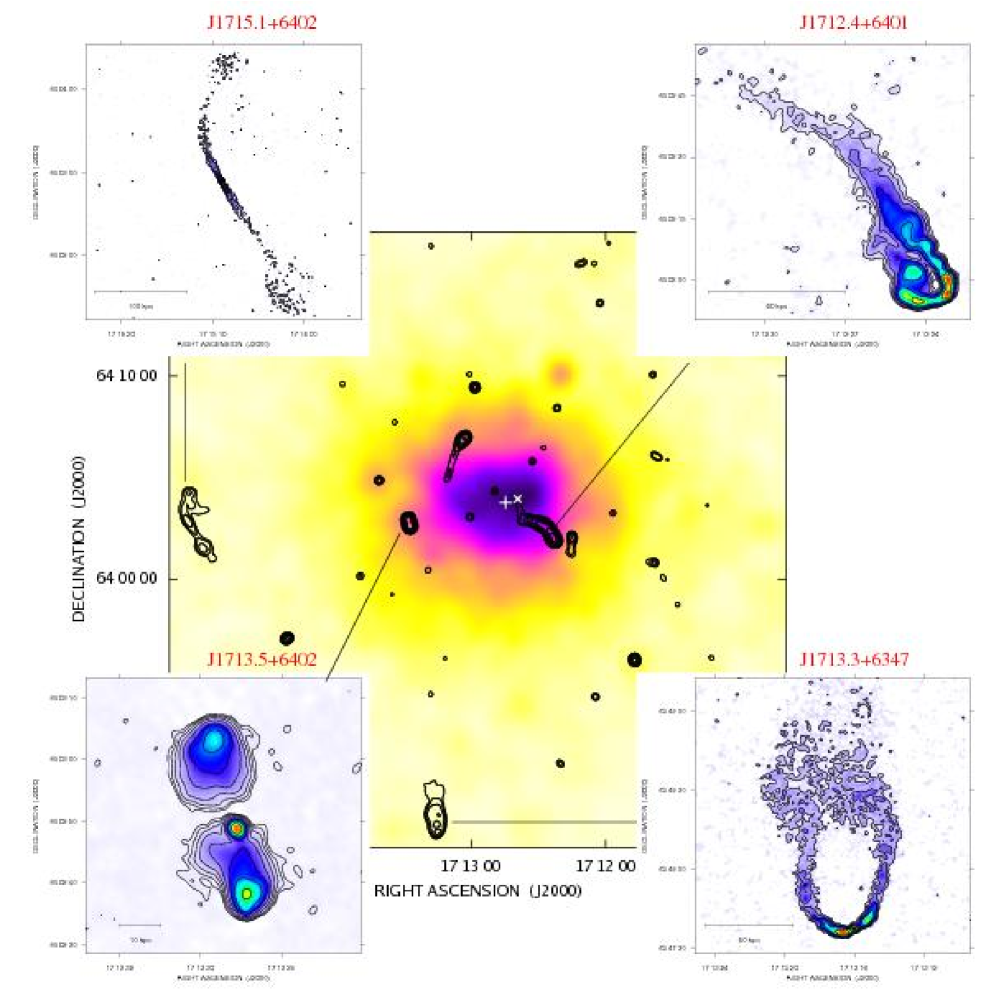
Figure 1: Radio contours of the A2255 cluster of galaxies obtained at 20 cm (Govoni et al. 2005) overlaid on the ROSAT X-ray image. The white symbols $+$ and $\times$ indicate the position of the cluster X-ray centroid and peak respectively. The radio image at 20 cm has a FWHM of $15^{\prime\prime}\times 15^{\prime\prime}$. The radio contours are: 0.4, 0.8, 1.6, 3.2, 6.4, 12.8, 25.6, and 51.2 mJy/beam. The sensitivity (1 $\sigma$) is 0.016 mJy/beam. For graphical reasons the first contour is at 25$\sigma$ therefore we see only the radio galaxies of the cluster while the low brightness, diffuse emissions (radio halo and relic) are not visible here. Pointed high resolution observations at 6 cm of four cluster radio galaxies are inset. The radio contours at 6 cm are: 0.06, 0.12, 0.24, 0.48, 0.96, 1.92, 3.84, and 7.68 mJy/beam. See Table 2 for more information (e.g. resolution, sensitivity, peak brightness) of these observations.

The four radio galaxies J1712.4+6401, J1713.3+6347, J1713.5+6402 and J1715.1+6402  have been investigated with multi-frequency, high-resolution, VLA observations. These sources have been selected on the basis of their high flux density ($>$80 mJy at 20 cm), extension, and the presence of polarized emission in the NVSS (Condon et al. 1998). The details of the observations are provided in Table 1. The sources were observed at two frequencies (4535/4885 MHz) within the 6 cm band and at two frequencies (8085/8465 MHz) within the 3.6 cm band, both in the B and C configurations. All observations were made with a bandwidth of 50 MHz.

The ($u,v$) data at the same frequencies but from different configurations were first handled separately and then combined. The source $1331+305$ (3C286) was used as the primary flux density calibrator, and as an absolute reference for the electric vector polarization angle. The phase calibrator was the nearby point source $1642+689$, observed at intervals of about 30 minutes. Calibration and imaging were performed with the NRAO Astronomical Image Processing System (AIPS), following standard procedures. Self-calibration was applied to remove residual phase variations.

Total intensity images $I$ have been produced by averaging the two frequencies in the same band while $U$ and $Q$ images have been obtained for each frequency separately. Images of polarized intensity $P=(Q^{2}+U^{2})^{1/2}$, fractional polarization $FPOL=P/I$ and position angle of polarization $\Psi=0.5\tan^{-1}(U/Q)$ were derived from the $I$, $Q$ and $U$ images.

3 Total intensity and polarization properties

Fig. 1 shows the contour image of A2255 (Govoni et al. 2005) at 20 cm overlaid onto the ROSAT PSPC image of the cluster. The X-ray image is in the band 0.5-2 keV and has been obtained from the ROSAT public archive by binning the photon event table in pixels of 15^′′ and by smoothing the image with a Gaussian of $\sigma=30^{\prime\prime}$. The centroid of the X-ray emission is approximately at RA(J2000)=$17^{h}12^{m}45^{s}$, DEC(J2000)=64^∘03^′54^′′(Feretti et al. 1997). The X-ray peak is shifted to the West with respect to this position. The large field of view of the radio image shows the location of the cluster radio galaxies with respect to the gas density distribution. For clarity the first radio contour is at 25$\sigma$. Therefore we see only the radio galaxies of the cluster while the low brightness diffuse emissions (radio halo and relic) are not visible here.

The high resolution (FWHM $\simeq$ 2^′′$\times$2^′′) images obtained at 6 cm for the four radio galaxies analyzed in this work are inset in Fig. 1. The sources are located at different distances from the cluster center which allows, through the study of their RM (presented in Sect. 4), the cluster magnetic fields to be estimated along different lines-of-sight.

Fig. 2 shows the high resolution (FWHM $\simeq$ 1^′′$\times$1^′′) observations in the 3.6 cm band for the four sources overlaid on the DSS2 red plate. Every source has a clear optical counterpart and all are classified as cluster radio galaxies on the basis of the optical spectroscopy analysis (Miller & Owen 2003; Yuan et al. 2003).

The relevant parameters of the radio images at high resolution are listed in Table 2.

In the following we give a brief description of the individual sources. In the radio images presented in Figs. 3 $-$ 6 we restored the maps at different frequencies with the same beam (2^′′$\times$2^′′). The relevant parameters of these total and polarization intensity images are listed in Table 3. The intensity and polarized flux densities were obtained, after the primary beam correction, by integrating in the same area the $I$ and $P$ surface brightness, respectively, down to the noise level. In Figs. 3 $-$ 6 contours represent total intensity while vectors represent the orientation of the projected E-field and are proportional in length to the fractional polarization. In the fractional polarization images, pixels with error greater than $10\%$ were blanked. The fractional polarization values given in the following subsections are calculated in the regions where the error is less than $10\%$.

Figure 2: Radio contours at 3.6 cm of four cluster radio galaxies overlaid on the DSS2 red plate (J1712.4+6401, J1713.3+6347, J1713.5+6402 and J1715.1+6402, from left to right). The radio contours are: 0.04, 0.08, 0.16, 0.32, 0.64, 1.28, 2.56, and 5.12 mJy/beam. See Table 2 for more information (e.g. resolution, sensitivity, peak brightness) of these observations.

Table 2: Total intensity images at high resolution (see Figs. 1 $-$ 2).

Source	$\lambda$	Beam	$\sigma$(I)	Peak
	(cm)	(′′)	(mJy/beam)	(mJy/beam)
J1712.4+6401	3.6	1.07$\times$0.97	0.014	1.9
′′	6	1.94$\times$1.75	0.019	3.2
J1713.3+6347	3.6	1.09$\times$1.06	0.013	2.2
′′	6	1.99$\times$1.82	0.018	2.4
J1713.5+6402	3.6	1.19$\times$1.02	0.014	11.6
′′	6	2.11$\times$1.82	0.021	12.8
J1715.1+6402	3.6	1.05$\times$1.03	0.013	3.2
′′	6	1.82$\times$1.78	0.016	3.5
Col. 1: Source; Col. 2: Observation wavelength; Col. 3: Beam;
Col. 4: RMS noise of the I image; Col. 5: Peak brightness.

Table 3: Total and polarization intensity radio images restored with a beam of 2^′′(see Figs. 3 $-$ 6).

Source	$\lambda$	Beam	$\sigma$(I)∗	$\sigma$(Q)∗	$\sigma$(U)∗	Peak brightness	Flux density	Pol. flux
	(cm)	(′′)	(mJy/beam)	(mJy/beam)	(mJy/beam)	(mJy/beam)	(mJy)	(mJy)
J1712.4+6401	3.6	2.0$\times$2.0	0.015	0.018	0.017	2.8	49.5	9.5
′′	6	′′	0.019	0.020	0.020	3.5	86.0	13.0
J1713.3+6347	3.6	′′	0.014	0.016	0.016	2.3	37.0	8.0
′′	6	′′	0.018	0.020	0.020	2.4	64.5	10.5
J1713.5+6402	3.6	′′	0.014	0.017	0.018	11.6	87.0	10.0
′′	6	′′	0.021	0.024	0.022	12.7	123.5	11.5
J1715.1+6402	3.6	′′	0.014	0.017	0.015	3.5	26.0	2.0
′′	6	′′	0.016	0.020	0.021	3.5	43.5	2.0
Col. 1: Source; Col. 2: Observation wavelength; Col. 3: Beam; Col. 4, 5, 6: RMS noise of the I, Q, U images;
∗ Note that while the I images have been obtained by averaging the two IFs in the same band, the Q and U images have been obtained for each
IF separately. Here we give the values of $\sigma$(Q) and $\sigma$(U) for the frequencies 8465 MHz and 4535 MHz at 3.6 cm and 6 cm respectively.
Col. 7: Peak brightness; Col. 8: Flux density; Col. 9: Polarized flux density (for the frequencies 8465 MHz and 4535 MHz at 3.6 cm and 6 cm respectively.)

3.1 J1712.4+6401

The source has a narrow-angle tail structure and it is located in projection quite near to the cluster center (see Fig. 1). The images show an unresolved core, in the position RA(J2000)=17^h12^m23^s, DEC(J2000)=64^∘01^′57^′′, South-West of the cluster center, and a long tail elongated North-East in the direction of the cluster X-ray centroid. The maximum projected angular size of the source at 6 cm is about 70^′′($\simeq$105 kpc) but it appears much more extended in our previous observation at 20 cm (2.5^′). At 3.6 cm only the brightest emission of the tail is detected.

Fig. 3 shows the polarization images of the source with an angular resolution of $2^{\prime\prime}\times 2^{\prime\prime}$. The source is strongly polarized both at 6 cm and 3.6 cm with a mean fractional polarization of about 14% and 12.5% respectively. In the core the fraction polarization is 2% at 6 cm and 4% at 3.6 cm and increases along the tail.

3.2 J1713.3+6347

This narrow-angle tail radio galaxy is located in the southern part of the cluster far from the center (see Fig. 1). From the compact component, in the position RA(J2000)=17^h13^m16^s, DEC(J2000)=63^∘47^′37^′′  two jets emanate and then bend to the north. The maximum projected angular size at 6 cm is about 90^′′  ($\simeq$135 kpc) but the source appears much more extended at 20 cm ($\simeq$3^′). At 3.6 cm only the brightest emission of the jets have been detected.

Fig. 4 shows the polarization images of the jets with an angular resolution of $2^{\prime\prime}\times 2^{\prime\prime}$. The sensitivity of the observations reveal significant polarization only in the inner parts of the jets up to a distance of about 15^′′($\simeq$20 kpc) from the core. The mean fractional polarization for the source is about 11% at 6 cm and 14% at 3.6 cm. In the core the fraction polarization is 2% at 6 cm and 0.4% at 3.6 cm. The jet on the east shows a lower fractional polarization (10% and 12% at 6 cm and 3.6 cm respectively) than the jet on the west (16% and 23% at 6 cm and 3.6 cm respectively).

3.3 J1713.5+6402

The source has a total extension of about 35^′′ ($\simeq$50 kpc) and a double structure with an unresolved core in the position RA(J2000)=17^h13^m29^s, DEC(J2000)=64^∘02^′49^′′(see Fig. 1).

Fig. 5 shows the polarization images of the source at 6 cm and 3.6 cm with an angular resolution of $2^{\prime\prime}\times 2^{\prime\prime}$. The mean fractional polarization is $\simeq$11% at 6 cm and $\simeq$13% at 3.6 cm. The fraction polarization of the core is 2% at 6 cm and 3% at 3.6 cm while the lobes are polarized at similar levels.

3.4 J1715.1+6402

This wide-angle tail source, located in the periphery of the cluster (see Fig. 1), is very extended with a size of about 3.5^′at 20 cm. The maximum projected angular size at 6 cm is about 200^′′  ($\simeq$300 kpc) but the low surface brightness lobes are only marginally detected at 6 cm and completely missed at 3.6 cm where only the first 30^′′ (45 kpc) of the jets are visible.

An unresolved component is located in the position: RA(2000)=17^h15^m09^s,DEC(2000)=64^∘02^′54^′′. Twin low brightness oppositely directed jets emanate from the core to the north-east and south-west. After 40^′′ (60 kpc) the north-east jet bends to the west toward the X-ray centroid while the other jet remains straight.

Fig. 5 shows the polarization images of the central part of the source with an angular resolution of $2^{\prime\prime}\times 2^{\prime\prime}$. We detect polarization only in the core and in the inner arcseconds of the jets. In the core the fraction polarization is 0.6% at 6 cm and 2% at 3.6 cm while in both jets it is about 14% at 6 cm. The polarization in the northern jet at 3.6 cm is below the sensitivity of the present observation while in the southern jets it is 12%.

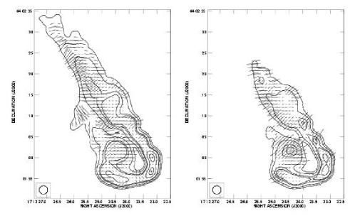
Figure 3: Source J1712.4+6401: Left: Total intensity contours and polarization vectors at 6 cm (4535 MHz). Right: Total intensity contours and polarization vectors at 3.6 cm (8465 MHz). The angular resolution is $2.0^{\prime\prime}\times 2.0^{\prime\prime}$. Contour levels are drawn at:$-$0.2, 0.2, 0.4, 0.8, 1, 2, 3, and 3.5 mJy/beam. The lines give the orientation of the electric vector position angle (E-field) and are proportional in length to the fractional polarization ($1^{\prime\prime}\simeq 16.7$%).

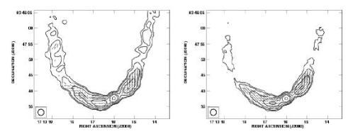
Figure 4: Source J1713.3+6347: Left: Total intensity contours and polarization vectors at 6 cm (4535 MHz). Right: Total intensity contours and polarization vectors at 3.6 cm (8465 MHz). The angular resolution is $2.0^{\prime\prime}\times 2.0^{\prime\prime}$. Contour levels are drawn at: $-$0.1, 0.1, 0.15, 0.3, 0.6, 1, and 2 mJy/beam. The lines give the orientation of the electric vector position angle (E-field) and are proportional in length to the fractional polarization ($1^{\prime\prime}\simeq 16.7$%).

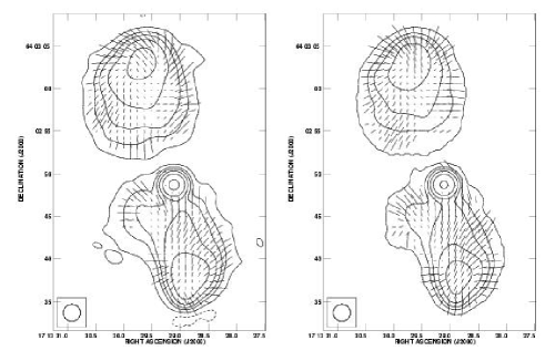
Figure 5: Source J1713.5+6402: Left: Total intensity contours and polarization vectors at 6 cm (4535 MHz). Right: Total intensity contours and polarization vectors at 3.6 cm (8465 MHz). The angular resolution is $2.0^{\prime\prime}\times 2.0^{\prime\prime}$. Contour levels are drawn at: $-$0.1, 0.1, 0.5, 1, 2, 4, and 10 mJy/beam. The lines give the orientation of the electric vector position angle (E-field) and are proportional in length to the fractional polarization ($1^{\prime\prime}\simeq 16.7$%).

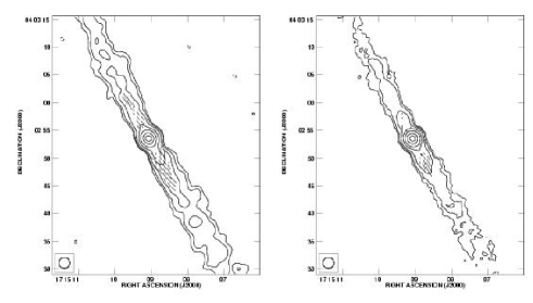
Figure 6: Source J1715.1+6402: Left: Total intensity contours and polarization vectors at 6 cm (4535 MHz). Right: Total intensity contours and polarization vectors at 3.6 cm (8465 MHz). The angular resolution is $2.0^{\prime\prime}\times 2.0^{\prime\prime}$. Contour levels are drawn at: $-$0.06, 0.06, 0.1, 0.2, 0.5, 1, 2, and 3 mJy/beam. The lines give the orientation of the electric vector position angle (E-field) and are proportional in length to the fractional polarization ($1^{\prime\prime}\simeq 16.7$%).

4 Rotation measure images

Polarized radiation from cluster and background radio galaxies may be rotated by the Faraday effect if magnetic fields are present in the intra-cluster medium. In this case, the observed polarization angle ($\Psi_{Obs}$) at a frequency $\nu$ is connected to the intrinsic polarization angle ($\Psi_{int}$) through:

$$\Psi_{Obs}(\nu)=\Psi_{int}+(c/\nu)^{2}\times RM$$ (1)

where the Rotation Measure (RM) is related to the electron density ($n_{e}$), the magnetic field along the line-of-sight ($B_{\parallel}$), and the path-length (L) through the intracluster medium according to:

$$RM_{\rm\leavevmode\nobreak\ [rad/m^{2}]}=812\int_{0}^{L_{[kpc]}}n_{e\leavevmode\nobreak\ [cm^{-3}]}B_{\parallel\leavevmode\nobreak\ [\mu G]}dl$$ (2)

We derived the rotation measure images, at 2^′′  resolution, of the four sources using the polarization angle maps $\Psi_{Obs}$ at the frequencies 4535, 4885, 8085 and 8465 MHz. The Faraday RM images were obtained by performing a fit of the polarization angle images at each pixel as a function of $\nu^{-2}$ (see Eq.1) using the algorithm PACERMAN (Polarization Angle CorrEcting Rotation Measure ANalysis) by Dolag et al. (2005). Instead of solving the n$\pi$-ambiguity for each pixel independently, the algorithm solves the n$\pi$-ambiguity for a high signal-to-noise region and uses this information to assist computations in adjacent low signal-to-noise areas.

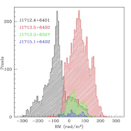
Figure 8: Histograms of the rotation measure images for all significant pixels.

Fig. 7 shows the total intensity contours at 3.6 cm overlaid on the RM images of the four cluster galaxies. The RM values range from about $-$300 rad/m² up to 250 rad/m² and reveal patchy structures with RM fluctuations down to scales of a few kpc. Fig. 8 shows the histograms of the RM distribution for the four sources. Due to the very low number of reliable RM pixels in J1715.1+6402 this source will not be considered in the following statistical analysis. Table 4 reports, for the other three sources sorted by distance from the X-ray centroid, the mean value $\langle{\rm RM}\rangle$  the root mean square $\sigma_{\rm RM}$ and the maximum absolute value $\arrowvert{\rm RM_{max}}\arrowvert$ of the RM distribution. These data are not corrected for the Galactic contribution which is likely negligible. A2255 in galactic coordinates is located at lon=93.97^∘and lat=$+34.95$^∘  and based on the average RM for extragalactic sources published by Simard-Normandin et al. (1981), the RM Galactic contribution in the region occupied by A2255 is expected to be about $-6$ rad/m².

Our data suffer from two kinds of uncertainty. The first uncertainty is related to the fit and takes into account the presence of errors in the measurements. In the RM images all the pixels with an error in the fit greater than 40 rad/m² were blanked. This ensures that at all frequencies we always consider pixels with an error in polarization angle lower than 10^∘  (see Eq. 1). The mean fit error calculated in the images is about 20 rad/m² for J1713.5+6402 and about 30 rad/m² for J1712.4+6401 and J1713.3+6347. The second source of error is the statistical error. Ideally one would determine the parameters of the RM distribution by investigating an area as large as possible. The morphology of sources and the presence of blanked pixels in the RM images introduce a further uncertainty in this determination. This uncertainty is particularly strong in sources where the reliable RM pixels are present in a small number of observing beams $N$ (see Table 4). The statistical error has been calculated to be about 10 and 5 rad/m² for the $\langle{\rm RM}\rangle$  and $\sigma_{\rm RM}$ respectively in J1713.5+6402 and about 15 and 10 rad/m² for the $\langle{\rm RM}\rangle$  and $\sigma_{\rm RM}$  respectively in the other two sources.

As found in other studies (Feretti et al. 1999, Taylor et al. 2001, Govoni et al. 2001a) aimed to study the cluster magnetic field by sampling the RM of extended radio galaxies located in the same cluster of galaxies, the most striking result is the trend of the RM values with distance from the cluster center. The innermost source, J1712.4+6401, has the highest $\sigma_{\rm RM}$  and $\arrowvert\langle{\rm RM}\rangle\arrowvert$. The source J1713.5+6402, located at about 1 core radius from the cluster center, shows considerably lower RM values. Finally, the peripheral source J1713.3+6347 shows a $\sigma_{\rm RM}$  consistent with its uncertainty but still has a significant $\langle{\rm RM}\rangle$.

The RM results are in agreement with the interpretation that the external Faraday screen is the same for all the sources, i.e. the decreasing radial profile of the RM data may be due to the intracluster medium of A2255, whose differential contribution depends on how much magneto-ionized medium is crossed by the polarized emission. Thus the data are consistent with the existence of a magnetic field associated with the intracluster medium.

The RM structures on small scales can be explained by the fact that the cluster magnetic field fluctuates on scales smaller than the size of the sources. On the other hand, the RM distribution with a non-zero mean indicate that the magnetic field fluctuates also on scales larger than the radio sources. Therefore to study in detail the cluster magnetic field properties it seems necessary to consider cluster magnetic fields models where both small and large scale coexist.

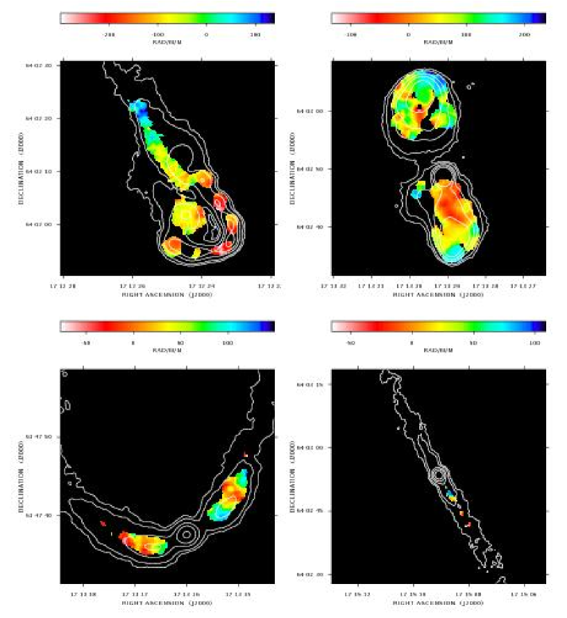
Figure 7: Images of the rotation measure computed using the polarization angle maps at the frequencies 4535, 4885, 8085 and 8465 MHz with a resolution of 2^′′. Contours refer to the total intensity images at 3.6 cm. Contour levels are: 0.06, 0.15, 0.5, 1, and 2 mJy/beam.

Table 4: Rotation measure.

Source	Centroid Dist.	$<{\rm RM}>$	$\sigma_{RM}$	$\arrowvert{\rm RM_{max}}\arrowvert$	N
	(kpc)	(rad/m2)	(rad/m2)	(rad/m2)	(Beams)
J1712.4+6401	315	$-$81	79	300	29
J1713.5+6402	450	67	59	236	41
J1713.3+6347	1570	36	42	149	6
Col. 1: Source; Col. 2: Projected distance from the X-ray centroid; Col. 3: Mean of the RM distribution;
Col. 4: RMS of the RM distribution. Col. 5: Maximum absolute value of the RM distribution;
Col. 6: Number of independent beams in the RM images.

5 The FARADAY tool

An analysis of the rotation measure of radio sources sampling different lines-of-sight across the cluster, together with an X-ray observation of the intracluster gas, can be used to derive information on the strength and structure of the cluster magnetic field. Complementary information on the cluster magnetic field can be derived by analyzing the radio halo emission. In particular, for a given distribution of the relativistic electrons in a cluster, different magnetic field models will generate very different total intensity and polarization brightness distributions for the radio halo emission. For those clusters containing a radio halo, a realistic magnetic field modeling should be able to explain both the small scale fluctuations seen in the RM images of cluster radio galaxies, and the morphology and polarization of the large scale diffuse emission.

The FARADAY tool, described in Murgia et al. (2004), permits an investigation of cluster magnetic fields by comparing the observations with simulated RM and radio halo images, obtained by considering 3-dimensional multi-scale cluster magnetic field models. We applied this method to A2255 with the aim of finding the optimal magnetic field strength and structure capable of describing both the high resolution RM images presented in this work and the large scale polarized features visible in the radio halo of A2255 (Govoni et al. 2005).

There are a number of quantities that are critical in our modeling, these are: the gas density distribution of the thermal electrons, the characterization of the magnetic field fluctuations and radial scaling, the energy density distribution of the synchrotron electrons.

For the distribution of the thermal electron gas density in A2255 we assumed a standard $\beta$-model profile:

$$n_{\rm e}(r)=n_{\rm 0}(1+r^{2}/r^{2}_{\rm c})^{-3\beta/2}$$ (3)

where $r$, $n_{\rm 0}$ and $r_{\rm c}$ are the distance from the cluster X-ray centroid, the central electron density, and the cluster core radius, respectively. The gas density distribution has been taken as derived from the ROSAT X-ray observations of Feretti et al. (1997), rescaled to our chosen cosmology ($r_{\rm c}$=432 kpc, $n_{\rm 0}=$2.05$\times$10^-3 cm^-3, $\beta$=0.74).

We considered different power law cluster magnetic field power spectrum models:

$$|B_{k}|^{2}\propto k^{-n}$$ (4)

in a 3-dimensional cubical box. We used a grid of 1024³ pixels in size which has the necessary resolution to sample the magnetic field power spectrum on a spatial scale ranging from $\Lambda_{\rm min}=4$ kpc up to $\Lambda_{\rm max}=512$ kpc. Observations reveal RM fluctuations on small scales supporting the choice for $\Lambda_{\rm min}$. The exact value of $\Lambda_{\rm max}$ is more uncertain, however the presence of ordered polarized filaments in the radio halos of A2255 indicates that, in the case of this cluster, the magnetic field fluctuates up to such large scales.

We adopted a magnetic field distribution decreasing from the cluster center according to:

$$\langle\mathbf{B}\rangle(r)=\langle\mathbf{B}\rangle_{\rm 0}\cdot(1+r^{2}/r_{\rm c}^{2})^{-3\mu/2}$$ (5)

where $\langle\mathbf{B}\rangle_{\rm 0}$ is the mean magnetic field at the cluster center. In order to estimate the index $\mu$, we first compared the $\sigma_{\rm RM}$ and the intracluster X-ray surface brightness, $S_{\rm X}$, at the location of each radio galaxy (Dolag et al. 2001). In the case of a beta model, the index $\mu$ is related to the slope, $\alpha$, of the $\sigma_{\rm RM}\propto S_{\rm X}^{\alpha}$ correlation through $\mu=(2\alpha-1)\cdot(\beta-1/6)$, see also Murgia et al. (2004). In the case of the three radio galaxies in A2255 the fit of the $\sigma_{\rm RM}-S_{\rm X}$ correlation yields $\alpha=0.6\pm 0.5$. The value of $\mu$ obtained with this method is indeed rather uncertain and lies in the range from $-$0.4 to 0.7. We thus estimated $\mu$ by comparing $S_{\rm X}$ and radio halo surface brightness at increasing radial distance from the cluster center (Govoni et al. 2001b). In A2255 it is observed a linear correlation between these two quantities, indicating that thermal and non-thermal (relativistic particles and magnetic fields) energy densities could have the same radial scaling. Therefore in the simulations we adopted $\mu=\beta/2$=0.37 which corresponds to a magnetic field whose energy density decreases in the same way as the gas energy density.

Provided the distribution of the thermal electrons and the magnetic field model described above we simulated the RM by integrating Eq. 2 along the line-of-sight.

To simulate the radio halo emission at each point of the computation grid we calculated the synchrotron emissivity by convolving the emission spectrum of a single relativistic electron with the particle energy distribution of an isotropic population of relativistic electrons whose distribution follows:

$$N(\epsilon,\theta)=N_{\rm 0}\epsilon^{-\delta}(\sin\theta)/2$$ (6)

where $\epsilon$ and $\theta$ are the electron’s energy and the pitch angle between the electron’s velocity and the direction of the magnetic field, respectively (see also Murgia et al. 2004).

The energy density of the relativistic electrons is:

$$u_{\rm el}=\int_{\epsilon_{\rm min}}^{\epsilon_{\rm max}}N(\epsilon)\epsilon d\epsilon$$ (7)

where $\epsilon_{\rm min}$ and $\epsilon_{\rm max}$ are the low and high energy cut offs of the energy spectrum, respectively.

In our model the magnetic field energy density $u_{\rm B}=B^{2}/8\pi$ and $u_{\rm el}$ are in equipartition at every point in the cluster, therefore both energy densities have the same radial decrease. We adopted an electron energy spectral index $\delta=3$ and a Lorentz factor for the high-energy cutoff of the electron distribution $\gamma_{\rm max}=1.5\times 10^{4}$. The resulting radio halo emission spectrum is roughly consistent with the radio spectral index map (not shown, Govoni et al. in preparation) obtained by combining our radio halo image at 1.4 GHz (Govoni et al. 2005) with the image at 327 MHz (Feretti et al. 1997). With $\delta=3$ we have $u_{\rm el}\simeq N_{\rm 0}/\gamma_{\rm min}$. The low-energy cutoff $\gamma_{\rm min}$ and $N_{\rm 0}$, are adjusted to guarantee the observed halo brightness and $u_{\rm el}=u_{\rm B}$. In practice we fix $\gamma_{\rm min}$=10 and let $N_{\rm 0}$ vary.

Below we present the simulated RM and radio halo images corresponding to two different variants of the above model. As a first approximation, we keep the power spectrum spectral index $n$ constant throughout the entire cluster (Sect.6). However, we find that this model does not reproduce the radio halo polarization level observed in A2255. To describe both the RM profiles and the radio halo polarization the data require a steepening of the power spectrum spectral index from the cluster center to the periphery and the presence of filamentary structures on large scales (i.e. a non-Gaussian magnetic field). In Sect.7 we will show that a model with these characteristics can better account for both the observed RM statistic and the radio halo polarization.

Table 5: Gas density and magnetic field parameters adopted in the simulations.

Grid sizea)	$1024^{3}$ pixels
Cellsize	1 pixel=2 kpc
Core radius	$r_{\rm c}$=432 kpc
Central density	$n_{\rm 0}$=2.05$\times$$10^{-3}$ cm-3
Beta	$\beta$=0.74
Magnetic field model	$|B_{k}|^{2}\propto k^{-n}$
Magnetic field radial profile slope	$\mu=0.37$
Magnetic field minimum scale	$\Lambda_{\rm min}$=4 kpc
Magnetic field maximum scale	$\Lambda_{\rm max}$=512 kpc
Central Mean magnetic field	free parameter
Power spectrum spectral index	free parameter (n=2-4)
a) To extend simulated RM images up to the source J1713.3+6347
the computational grid has been replicated at boundaries realizing a
field of view of 4096$\times$4096 kpc2

The computational grid, gas density, and magnetic field model parameters of the simulations are provided in Table 5. A grid size of $1024^{3}$ pixels with a cellsize of 2 kpc allows us to simulate a cluster field of view of 2048$\times$2048 kpc². The simulated magnetic field is periodic at the grid boundaries. Thus, to extend our RM simulations up to the source J1713.3+6347, the computational grid has been replicated realizing a field of view of 4096$\times$4096 kpc² (i.e. up to about one virial radius).

6 Constant magnetic field power spectrum slope

6.1 Simulated Rotation Measure images

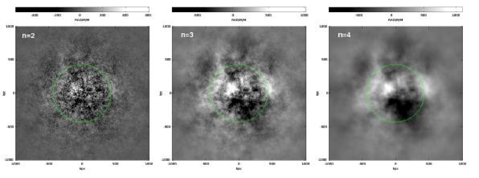
Figure 9: Simulated RM images for different values of the magnetic field power spectrum spectral index $n$. The three power spectra are normalized to have the same total magnetic field energy which is distributed over the range of spatial scales from 4 kpc up to 512 kpc. In these simulations the average field at the cluster center is $\langle\mathbf{B}\rangle$₀ $=2\leavevmode\nobreak\ \mu$G and its energy density decreases from the cluster center according to $B^{2}\propto n_{\rm e}(r)$. Each RM image shows a field of view of about $2\times 2$ Mpc. We performed the RM integration from the cluster center up to 4 Mpc along the line-of-sight. The circles represent the cluster core radius.

In Fig. 9 we show the central $2\times 2$ Mpc² region of the simulated RM images of A2255 for three different values of the magnetic field power spectrum spectral index, $n$=2, 3 and 4.

To obtain such images we performed the integration of Eq. 2 from the cluster center up to 4 Mpc along the line-of-sight using the magnetic field model described in the previous section. The three magnetic field power spectra are normalized to generate the same average magnetic field energy density. The average magnetic field strength at the cluster center is $\langle\mathbf{B}\rangle$${}_{\rm 0}=2\,\mu$G and its energy density decreases from the cluster center following the gas energy profile. The central magnetic field strength of this set of simulations provides the best fit to the observed RM radial profiles (see below). It is evident from Fig. 9 that the same cluster magnetic field energy density generates different magnetic field configurations with correspondingly different RM structures, for different values of the power spectrum spectral index.

RM images of the whole cluster, such as those presented in Fig. 9, cannot be observed in reality. However it is possible to derive the RM from limited regions of the cluster by observing radio sources located at different projected distances from the center as described in Sect. 4. The comparison of the observations with the simulations can constrain the magnetic field strength and power spectrum. In such a comparison the details of the three-dimensional structure of the radio sources are neglected, and the entire observed Faraday rotation is assumed to occur in the intracluster medium. The three radio galaxies considered in this work are cluster members. For what concerns their location along the line-of-sight, we followed two approaches. As first approximation, we supposed that the three galaxies lie on a plane perpendicular to the line-of-sight at the distance of the cluster center. The simulations shown in Fig. 9 reproduce such a situation. As an improvement, we extracted the Faraday depth of the simulated RM images randomly from the 3 dimensional distribution of bright member galaxies observed in A2255. We determined this trend by fitting with a King model the spatial galaxy distribution of the brightest spectroscopically confirmed member galaxies taken from Yuan et al. (2003). The fit, shown in Fig. 10, has been extended only to those members characterized by a red magnitude brighter than $M_{\rm R}<-21$ since radio galaxies usually populate this optical luminosity range (e.g. Govoni et al. 2000).

To compare directly the simulations with the observations we added to the simulated RM images a noise of 30 rad/m² (corresponding to the typical fit error in our data) and an offset of $-6$ rad/m² (representing the RM galactic contribution calculated in the direction of A2255). Therefore, in the peripheral regions of the simulated RM images, where the contribution of the cluster Faraday screen is negligible, we have $\sigma_{\rm RM}$$\simeq$30 rad/m² and $\langle{\rm RM}\rangle$$\simeq-6$ rad/m². These are the lower limits of our simulations.

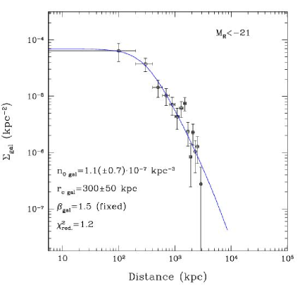
Figure 10: Spatial distribution of member galaxies in A2255 taken from Yuan et al. (2003). The solid line represents the fit of the King model $n_{\rm gal}=n_{\rm 0\,gal}(1+r^{2}/r_{\rm c\,gal}^{2})^{-\beta_{\rm gal}}$ to the data. We derived a central density of galaxies $n_{\rm 0\,gal}=1.1\pm 0.7\times 10^{-7}$ kpc^-3 and a core radius $r_{\rm c\,gal}=300\pm 50$ kpc. The $\beta_{\rm gal}$ parameter have been fixed to 3/2. The fit, has been extended only to those members characterized by a red magnitude brighter than $M_{\rm R}<-21$.

In Fig. 11 we compare the observed $\sigma_{\rm RM}$ and $\arrowvert\langle{\rm RM}\rangle\arrowvert$  with the expectation of the simulations (for $n=2,3,4$ and $\langle\mathbf{B}\rangle$₀ $=2\leavevmode\nobreak\ \mu$G, see below). The plotted data are those presented in Table 4. The error bars represent only the statistical errors discussed in Sect. 4 and do not account for fitting errors since those are already included in the simulated RM images. Since the observed $\sigma_{\rm RM}$  and $\langle{\rm RM}\rangle$  are calculated in limited regions over the radio galaxies, we have to sample the corresponding simulated values in regions of equivalent size. The expected radial trends have been obtained by covering the simulated RM images with a grid of rectangular boxes of $50\times 50$ kpc² in size. These boxes reproduce the regions covered by the RM images of the radio galaxies in A2255. Inside each box we calculated the values of $\sigma_{\rm RM}$ and $\arrowvert\langle{\rm RM}\rangle\arrowvert$ exactly as it would be done if they were real radio sources. Due to the random nature of the simulated magnetic field, the values of $\sigma_{\rm RM}$ and $\arrowvert\langle{\rm RM}\rangle\arrowvert$ at a given radial distance vary from box to box. However, the numerical simulations allow us to quantify this statistical variance. We calculated the mean and the dispersion of $\sigma_{\rm RM}$ and $\arrowvert\langle{\rm RM}\rangle\arrowvert$ values from all the boxes located at the same projected distance from the cluster center. The dark lines show the mean while the dark gray regions show the dispersion of the profiles calculated in the simulations shown in Fig. 9. The light gray regions represent the increase of the scatter of simulated RM in the case in which the location of the boxes along the line-of-sight is extracted randomly from the 3 dimensional distribution of galaxies in A2255. The horizontal dashed lines represent the lower limits of $\sigma_{\rm RM}$  and $\langle{\rm RM}\rangle$  caused by the presence of fitting errors and the RM galactic contribution.

Both the values of $\sigma_{\rm RM}$ and $\arrowvert\langle{\rm RM}\rangle\arrowvert$  depend linearly on the cluster magnetic field strength. The best fit of the simulated $\sigma_{\rm RM}$  radial profiles with respect to the $\sigma_{\rm RM}$  values observed in A2255 was obtained by considering a central magnetic field of about 2 $\mu$G. It reproduces quite well the observed $\sigma_{\rm RM}$  for each of the considered values of the magnetic field spectrum spectral index ($n$=2,3,4), as shown in the left panel of Fig. 11. The comparison between simulated and observed $\arrowvert\langle{\rm RM}\rangle\arrowvert$  (Fig. 11, right panels) allows us to constrain the value of the best index of the power spectrum. In order to quantify the relative goodness of the fit of the $\arrowvert\langle{\rm RM}\rangle\arrowvert$ profiles we calculated the sum

$$\chi^{2}=\Sigma\frac{({\arrowvert\langle{\rm RM}\rangle\arrowvert}_{\rm Sim}-{\arrowvert\langle{\rm RM}\rangle\arrowvert}_{\rm Obs})^{2}}{{\rm Scatter}_{\rm Sim}^{2}+{\rm Err}_{\langle{\rm RM}\rangle}^{2}}$$ (8)

where ${\rm Scatter}_{\rm Sim}$ and ${\rm Err}_{\langle{\rm RM}\rangle}$ represent the scatter of the simulations and the statistical $\arrowvert\langle{\rm RM}\rangle\arrowvert$ error, respectively.

A flat spectral index power spectrum, $n=2$, is ruled out since it predicts too low $\arrowvert\langle{\rm RM}\rangle\arrowvert$  for all three sources. A steep spectral index power spectrum, $n=4$, fits the outer source but predicts too much $\arrowvert\langle{\rm RM}\rangle\arrowvert$  for the two central sources. The model with $n=3$ agrees better with the data.

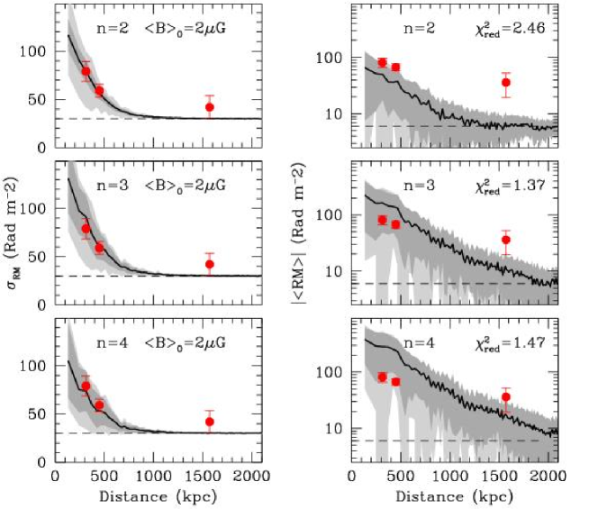
Figure 11: Comparison of $\sigma_{\rm RM}$ (left column panels) and $\arrowvert\langle{\rm RM}\rangle\arrowvert$ (right column panels) data of the three cluster radio galaxies (dots) with the simulated profiles (dark lines). The dark gray regions show the dispersion of the profiles calculated in the simulations shown in Fig. 9. The light gray regions represent the increase of the scatter of simulated RM in the case in which the Faraday depth of the simulated RM images is extracted randomly from the 3 dimensional distribution of galaxies in A2255. The horizontal dashed lines represent the lower limits of $\sigma_{\rm RM}$  and $\langle{\rm RM}\rangle$  caused by the presence of fitting errors and the RM galactic contribution. In the right panels the value of the reduced $\chi^{2}$ for two degree of freedom is also indicated.

6.2 Simulated radio halo images

We simulated the expected total intensity and polarization brightness distribution at 1.4 GHz, for a magnetic field strength $\langle B\rangle_{\rm 0}=$2 ${\rm\mu G}$ as found in the RM data.

In Fig. 12 we show the simulated radio halo brightness (contours) and fractional polarization (color) for the three different magnetic field spectral indices $n$=2, 3 and 4. For a direct comparison with the data (see Fig. 15 ; bottom right panel) these images have been convolved with a beam of 25^′′ (37.5 kpc) and the lowest contour level has been chosen to match the dynamic range of 10 as in the observations.

As in the case of the simulated RM images, the same cluster magnetic field energy density generates different magnetic field configurations with correspondingly different halo morphologies, for different values of the power spectrum spectral index, $n$. However, in this case these differences are even more evident given that the radio halo intensity depends upon the square of the magnetic field fluctuations.

Flat power spectrum indexes ($n=2$) give rise to a regular and smooth radio halo morphology. Increasing the spectral index, $n$, and thus the power on large scales, the radio halo becomes increasingly irregular. For $n=4$ the radio halo emission is confined to a few bright filaments. Again, the simulated radio halo corresponding to $n=3$ seems to better reproduce the observed morphology.

The internal depolarization of the radio halo emission is stronger where the RM is higher and where the magnetic field is tangled on small scales. Thus, as one would expect, we found that the degree of fractional polarization increases with increasing values of $n$ and decreases towards the cluster center (Murgia et al. 2004). In any case, one can observe significant polarized emission only from the outer layers of the halo observed along the line of sight paths that do not cross the cluster center. The maximum fractional polarization attained in this set of simulations at the outer halo edges ranges from 5%, for $n=2$, up to 9%, for $n=4$. These values are definitely lower than the values observed in the radio halo of A2255.

Therefore, our results seem to indicate that a single magnetic field power spectrum slope cannot account for both the observed RM and radio halo images. Even $n=3$, which gives a good results for the RM profiles and radio halo morphology, yields insufficient polarization levels.

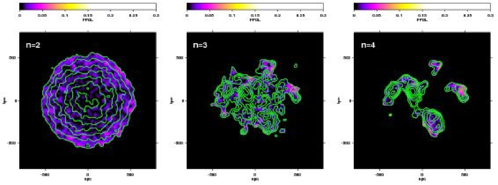
Figure 12: Simulated radio halo brightness (contours) and fractional polarization (color) for the three different magnetic field spectral indices $n$=2, 3 and 4. For a direct comparison with the data (Fig. 15; bottom right panel) these images have been convolved with a beam of 25^′′  (37.5 kpc) and the lowest contour level has been chosen to match the dynamic range of 10 as in the observations.

7 Variable magnetic field power spectrum slope

The results of the previous section suggest that the magnetic field power spectrum slope may change as a function of distance from the cluster center. The data require that much of the magnetic field energy density at the cluster center should be concentrated on small scales in order to account for the observed RM dispersion. On the other hand, to explain the highly polarized structures observed in the radio halo it is necessary that most of the magnetic field energy density is on large scales at the cluster periphery. This scenario is also consistent with the relatively large $\langle{\rm RM}\rangle$ of the most external radio galaxy J1713.3+6347 (see Fig. 11). We thus considered a magnetic field configuration whose power spectrum gradually steepens with increasing distance from the cluster center (see Fig. 13).

After a series of simulations, we found that the best global magnetic field is composed by the sum of:
i) a Gaussian, $n=2$, magnetic field whose intensity decays exponentially beyond the core radius and
ii) a non-Gaussian, $n=4$, magnetic field with $\Lambda_{\rm min}=32$ kpc and $\Lambda_{\rm max}=512$ whose intensity decays exponentially for $r<r_{\rm c}$. The values of $\Lambda_{\rm min}$ and $\Lambda_{\rm max}$ adopted for the outer field are roughly consistent with the observed width and length of the polarized radio halo filaments, respectively. We achieved the non-Gaussianity of the outer magnetic field fluctuations by exponentiating a ’parent’ Gaussian magnetic field with $n=4$.

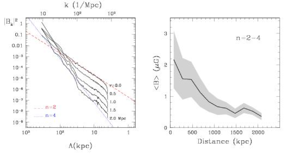
Figure 13: Left: magnetic field power spectra as a function of the distance from the cluster center for the variable magnetic field power spectrum slope model. The dashed and dotted reference lines have a slope of 2 and 4, respectively. Right: radial profile of the magnetic field strength. The solid line represents the average magnetic field strength while the gray region indicates the root mean square of the magnetic field fluctuations.

Non-Gaussian fields are characterized by a lower filling factor with respect to Gaussian random fields since magnetic field energy is more concentrated in filaments. The non-Gaussianity is indeed a necessary feature of the outer field since it allow us to enhance the field strength in the polarized filaments boosting their prominence. Moreover, the presence of large voids in the magnetic field ensures that the $\langle{\rm RM}\rangle$  over the two central radio galaxies is not exceeded as would happen for a Gaussian field with a similar power spectrum slope (see bottom left panel of Fig. 11).

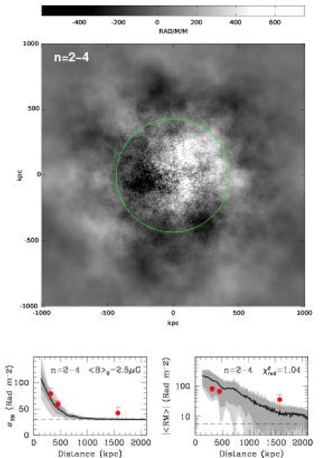
Figure 14: Top: simulated RM image as appears for a variable value of the magnetic field power spectrum spectral index $n=2-4$. In this simulation the average field at the cluster center is $\langle\mathbf{B}\rangle$₀ $=2.5\leavevmode\nobreak\ \mu$G and its energy density decreases from the cluster center according to $B^{2}\propto n_{\rm e}(r)$. The RM image shows a field of view of about $2\times 2$ Mpc. We performed the RM integration from the cluster center up to 4 Mpc along the line-of-sight. The circle represent the cluster core radius. Bottom: Comparison of $\sigma_{\rm RM}$ (left column panel) and $\arrowvert\langle{\rm RM}\rangle\arrowvert$ (right column panel) data of the three cluster radio galaxies (dots) with the simulated profiles (dark lines). The dark gray regions show the dispersion of the profiles calculated in the simulations. The light gray regions represent the increase of the scatter of simulated RM in the case in which the Faraday depth of the simulated RM images is extracted randomly from the 3 dimensional distribution of galaxies in A2255. The horizontal dashed lines represent the lower limits of $\sigma_{\rm RM}$  and $\langle{\rm RM}\rangle$  caused by the presence of fitting errors and the RM galactic contribution. In the right panel the value of the reduced $\chi^{2}$ for two degree of freedom is also indicated.

7.1 Simulated Rotation Measure images

The resulting cluster RM images and profiles, obtained with the same procedure described in Sect. 6.1, are shown in Fig. 14. The average magnetic field strength at the cluster center is 2.5 $\mu G$. The RM image shows that the small scale field fluctuations are stronger at the cluster center while the large scale magnetic field dominates at the periphery. The RM profiles shows that this model is able to reproduce both the $\sigma_{\rm RM}$  and the $\langle{\rm RM}\rangle$  of all three sources better than a constant magnetic field slope model can.

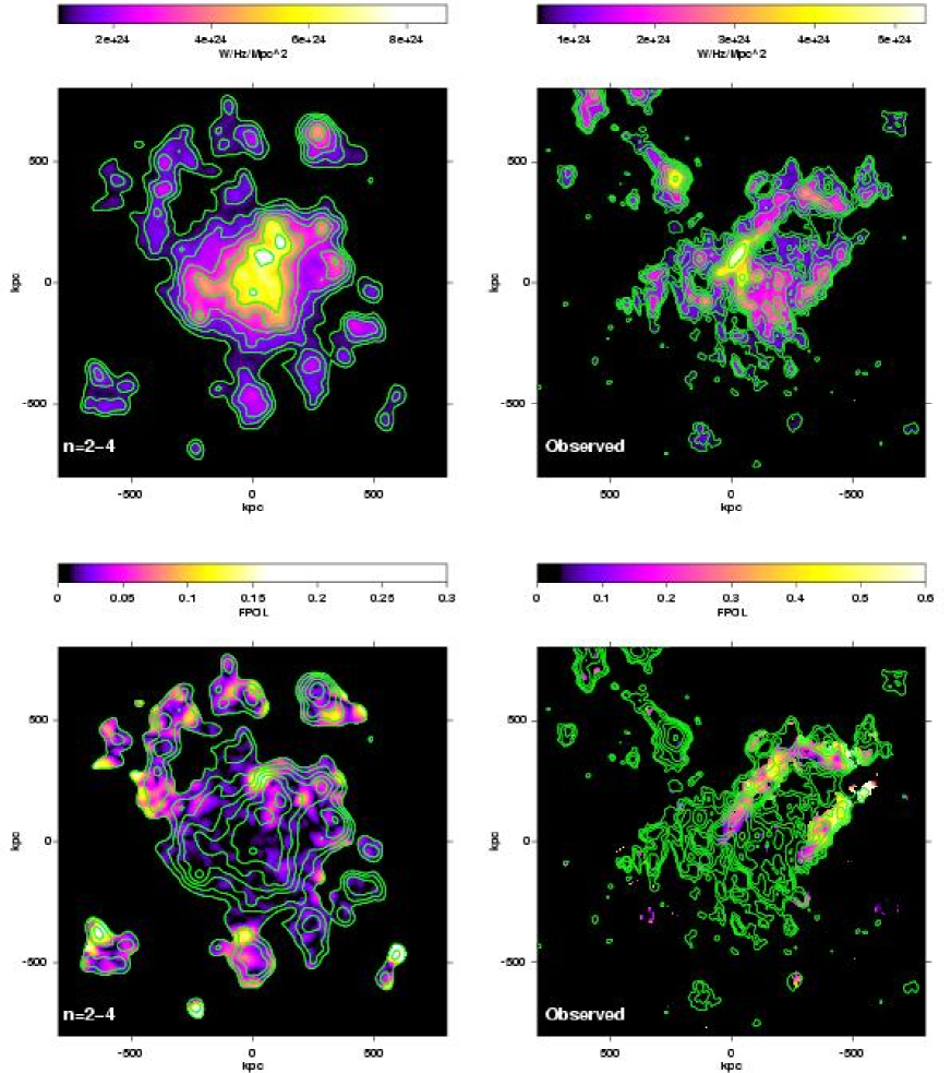
Figure 15: Top: Simulated (left panel) radio halo brightness for a variable magnetic field spectral index $n$=2-4. For a direct comparison with the data (right panel) this image has been convolved with a beam of 25^′′  (37.5 kpc) and the lowest contour level has been chosen to match the dynamic range of 10 as in the observations. Bottom: Simulated (left panel) radio halo brightness (contours) and fractional polarization (color) for the variable magnetic field spectral index $n$=2-4. For a direct comparison with the data see the right panel. Note that in the observed image of A2255 the radio galaxies have been subtracted and the emission of the peripheral radio relic is not in the field of view.

7.2 Simulated radio halo images

In Fig. 15, we present the observed radio halo total intensity and fractional polarization images (right panels) along with their simulated counterparts (left panels) generated by considering the magnetic field model outlined above. By comparing the total intensity images we are able to reproduce both the brightness level, the size, and the overall morphology of the halo. More importantly, the fractional polarization of the simulated filaments reaches values as high as 10%-20%. These values, although still somewhat lower than those observed, (the average polarization percentage in filaments is 30%), are substantially higher than those presented in the previous section and clearly represent an improvement over the model based on a constant slope $n$.

Note that with the same magnetic field strength we are able to explain both the RM data and the radio luminosity of the radio halo while keeping relativistic particle and field energy densities in equipartition. However, the equipartition magnetic field of the simulated radio halo calculated using standard formulas (Pacholczyk 1970) results in about 0.3 $\mu G$ over a 1Mpc³ volume (the same result obviously holds also for the observed radio halo since both have roughly the same size and luminosity). With such a magnetic field strength, which is lower than the average magnetic field of the simulations over the same volume $\langle B\rangle\simeq 1.2$  $\mu G$, it would be virtually impossible to fit the RM data, since the expected $\sigma_{\rm RM}$  and $\langle{\rm RM}\rangle$  profiles will be one order of magnitude lower than those shown in Fig.14. This problem is usually addressed in the literature as a discrepancy between the magnetic field strength estimated from the RM and that estimated from the minimum energy argument. In our simulation this problem is not present since most of the relativistic particles are at low energies and are undetectable at observable radio wavelengths. We do not claim that we have solved the aforementioned discrepancy. But we note that the classical equipartition estimate is critically dependent on the low energy cut-off of the electron energy spectrum for steep spectrum sources such as radio halos. Thus, until a precise knowledge of the low energy spectrum of the synchrotron electrons in radio halos can be reached, the equipartition estimates of the magnetic field strength in these radio sources should be used with caution.

In conclusion, we find that a magnetic field power spectrum whose slope steepen from the cluster center outwards provides a good description of the RM radial profiles and is able to reproduce both the luminosity and the fractional polarization of the radio halo, thus reconciling the magnetic field strength estimated obtained using these two complementary methods of analysis.

The fractional polarization of the observed radio halo is still higher than the simulated one. However, we do not exclude that more sophisticated magnetic field models, e.g. non-Gaussian random fields with ad-hoc correlated phases, can better reproduce the observed filamentary polarized structures.

We checked that the magnetic field radial profile adopted in our simulations, in particular the value of $\mu$, does not strongly affect the results.

8 Conclusions

We present new VLA observations at 3.6 and 6 cm for four polarized radio galaxies embedded in A2255, obtaining detailed RM images for three of them. The dispersion and the mean of the RM decrease with increasing distance from the cluster center. We analyze these data, together with the very deep radio halo image recently obtained by Govoni et al. (2005). Using the numerical approach described in Murgia et al. (2004), we simulate random 3-dimensional magnetic field models characterized by different power spectra and produce synthetic RM and radio halo images. By comparing the simulations with the data we investigate the strength and the power spectrum of the intra-cluster magnetic field fluctuations.

We find that a magnetic field power spectrum with a single spectral index is not suitable to reproduce both the rotation measure distribution of radio galaxies, and the radio halo polarization. The data require a steepening of the power spectrum spectral index from $n=2$, at the cluster center, up to $n=4$ at the cluster periphery and the presence of filamentary structures on large scale. This result seems to indicate that the magnetic field at the cluster center would be more dominated by small-scale structures, while at the periphery most of the magnetic field energy density is concentrated on the large-scale structures. A magnetic field with power spectrum steepening with radius is likely to reflect a complex behaviour of turbulence and motions in clusters. Subramanian et al. (2006) discuss the evolving turbulence due to dynamo action, and find that turbulence can coexist with ordered filamentary gas structure. Since turbulence is likely driven by a merger event, it may be expected that this driving is stronger in the cluster central region. In this case, turbulence in the peripheral regions can be in a more advanced stage of decay than at the cluster center. Since smaller scales decay first, and the integral scale of decaying turbulence increases with time, larger-scale magnetic field structures may be more easily present in the outer cluster region.

The average magnetic field strength at the cluster center is 2.5 $\mu G$. The field strength declines from the cluster center outward and the average magnetic field strength calculated over 1 Mpc³ is about 1.2 $\mu$G.

In conclusion, we find that the above magnetic field model provides a good description of the RM radial profiles and is able to reproduce both the luminosity and the fractional polarization of the radio halo, thus reconciling the magnetic field strength estimated using two complementary methods of analysis.

- (1) Burns, J.O., Roettiger, K., Pinkney, J., et al. 1995, ApJ 446, 583
- (2) Carilli, C.L. & Taylor, G.B. 2002, ARA&A, 40, 319
- (3) Clarke, T.E., Kronberg, P.P., Böhringer, H., 2001, ApJ 547, L111
- (4) Clarke, T.E.: 2004, Journal of Korean Astronomical Society, 37, 337
- (5) Condon J.J., Cotton W.D., Greisen E.W. et al., 1998, AJ 115, 1693
- (6) Dolag K., Schindler S., Govoni F., Feretti L., 2001, A&A 378, 777
- (7) Dolag, K., Bartelmann, M., Lesch, H., 2002, A&A 387, 383
- (8) Dolag, K., Vogt, C., Enßlin, T.A., 2005, MNRAS 358, 726
- (9) Enßlin T.A., Vogt C., 2003, A&A, 401, 835
- (10) Feretti, L., Böhringer, H., Giovannini, G., Neumann, D. 1997, A&A 317, 432
- (11) Feretti, L., Dallacasa, D., Govoni, F., Giovannini, G., Taylor, G.B., Klein, U., 1999, A&A 344, 472
- (12) Fusco-Femiano, R., Orlandini, M., Brunetti, G., Feretti, L., Giovannini, G., Grandi, P., Setti, G., 2004, ApJ 602, L73
- (13) Giovannini, G., Feretti, L., 2002, ASSL Vol. 272: Merging Processes in Galaxy Clusters, 197
- (14) Govoni, F., Falomo, R., Fasano, G., Scarpa, R. 2000, A&A, 353, 507
- (15) Govoni, F., Taylor, G.B., Dallacasa, D., Feretti, L., Giovannini, G., 2001a, A&A 379, 807
- (16) Govoni, F., Enßlin, T.A., Feretti, L., Giovannini, G., 2001b, A&A, 369, 441
- (17) Govoni, F., Feretti, L., 2004, International Journal of Modern Physics D 13, 1549
- (18) Govoni, F., Murgia, M., Feretti, L., Giovannini, G., Dallacasa, D., Taylor, G. B., 2005, A&A 430, L5
- (19) Harris, D.E., Kapahi, V.K., Ekers, R.D., 1980, A&AS 39, 215
- (20) Jaffe, W.J., Rudnick, L., 1979, ApJ 233, 453
- (21) Miller N.A., Owen F.N., 2003, AJ 125, 2427
- (22) Murgia M., Govoni F., Feretti L., Giovannini G., Dallacasa D., Fanti R., Taylor G.B., Dolag K., 2004, A&A 424, 429
- (23) Pacholczyk, A.G., Radio Astrophysics (Freeman, San Francisco, 1970)
- (24) Rephaeli, Y., Gruber, D., Arieli, Y., 2006, ApJ in press, astro-ph/0606097
- (25) Sakelliou, I., & Ponman, T. J., 2006, MNRAS 367, 1409
- (26) Simard-Normandin M., Kronberg P.P., Button S., 1981, ApJS 45, 97
- (27) Struble, M.F., Rood, H.J., 1999, ApJS, 125, 35
- (28) Subramanian K., Shukurov A., Haugen N.E.L., 2006, MNRAS 366, 1437
- (29) Taylor G.B., Govoni F., Allen S., Fabian A.C., 2001, MNRAS 326, 2
- (30) Vikhlinin, A., Markevitch, M., 2002, Astronomy Letters, 28, 495
- (31) Yuan, Q., Zhou, X., & Jiang, Z. 2003, ApJS, 149, 53
- (32) Yuan, Q., Zhao, L., Yang, Y., et al. 2005, AJ, 130, 2559