On the dynamics of radiative zones in rotating stars

Abstract

In this lecture I try to explain the basic dynamical processes at work in a radiative zone of a rotating star. In particular, the notion of baroclinicity is thoroughly discussed. Attention is specially directed to the case of circulations and the key role of angular momentum conservation is stressed. The specific part played by viscosity is also explained. The old approach of Eddington and Sweet is reviewed and criticized in the light of the seminal papers of Busse 1981 and Zahn 1992. Other examples taken in the recent literature are also presented; finally, I summarize the important points.

1 Introduction

It is well known since the seminal work of von Zeipel (1924) that radiative zones of a rotating star cannot be at rest; in other words no hydrostatic solution exists in any frame: some shearing flow must occur. The importance of such flows comes from their relation with the abundances of elements at the surface of stars. Indeed, the interpretation of these observations requires the understanding of the close relation between rotation and mixing, namely the transport of elements in radiative zones, which, without rotation would be a pure diffusive process.

As any fluid dynamical process, flows in rotating radiative zones are governed by PDE and therefore difficult to evaluate in a simple way. This is the reason why much misleading work has been published on the subject, especially under the title of the Eddington-Sweet circulation. In this lecture I would like to present as clearly as possible the dynamical processes at work in a rotating radiative zone and explain why the idea of Eddington-Sweet circulation is a misunderstanding of the problem.

2 Dynamical ingredients

2.1 Equations of motion

Unlike many problems in fluid mechanics where flows are produced by a given force field (just think for instance to the case of a river whose water flows down thanks to gravity), flows in rotating radiative zones are the result of a mismatch between two force fields, namely the pressure gradient and the gravity force. This mismatch gives birth to a torque field, the baroclinic torque, which locally produces vorticity and thus fluid motion. Before discussing this matter, it is however necessary to have a look to the equations of motion and especially to the momentum equation in a rotating frame; this equation reads:

$$\rho\left(\frac{D\vec{v}}{Dt}+\underbrace{2\vec{\Omega}\wedge\vec{v}}_{\rm I}+\underbrace{\Omega^{2}\vec{s}}_{\rm II}\right)=-{\rm NewA}P+\underbrace{\rho\vec{g}}_{\rm III}$$

where we discarded viscosity. Terms I, II, III are specific of this problem; they are respectively for:

• The Coriolis acceleration $2\vec{\Omega}\wedge\rho\vec{v}$ which insures conservation of angular momentum.

• The centrifugal acceleration $-\Omega^{2}\vec{s}$ which is at the origin of baroclinicity.

• The gravity force which transform a density fluctuation into motion.

2.2 The wave zoo

Before diving into the heart of the subject, it is useful to recall the waves able to propagate in a rotating radiative zone. There are three sorts of waves of that kind: the acoustic, the gravity and the inertial waves.

2.2.1 The acoustic waves

In a uniform medium acoustic waves are described by

$$\left\{\begin{array}[]{l}\rho_{0}\frac{\partial\vec{v}}{\partial t}=-{\rm NewA}p^{\prime}\\ \frac{\partial\rho^{\prime}}{\partial t}+\rho_{0}\mathop{\hbox{div}}\nolimits\vec{v}=0\\ \frac{\partial s^{\prime}}{\partial t}=0\end{array}\right.$$ (1)

namely momentum, mass and entropy conservation. Note that for such waves $\partial_{t}\rho^{\prime}$ is an essential term. Equations have been linearized and 0-index terms refer to the background state. The dispersion relation of these waves, namely $\omega=c_{s}k$, where $c_{s}$ is the speed of sound, shows that acoustic frequencies have no upper limit. But they have a lower limit given by a $k_{\rm min}$ coming from the finite size of the container (the star !).

2.2.2 The gravity waves

While acoustic waves exist because of the pressure field, the restoring force of gravity waves is the buoyancy. Compressibility is unnecessary and therefore density can be kept constant except when it yields buoyancy (this is the Boussinesq approximation in a very short description). In its simplest form, the system of equation describing these waves is

$$\left\{\begin{array}[]{l}\rho_{0}\frac{\partial\vec{v}}{\partial t}=-{\rm NewA}p^{\prime}+\rho^{\prime}\vec{g}\\ \mathop{\hbox{div}}\nolimits\vec{v}=0\\ \frac{\partial T^{\prime}}{\partial t}+\vec{v}\cdot{\rm NewA}T_{0}=0\\ \rho^{\prime}/\rho_{0}=-\alpha T^{\prime}\end{array}\right.$$ (2)

where $\alpha$ is the dilation coefficient. Note that temperature, which could be replaced by any other scalar field (like concentration for instance), needs to be non-uniform.

Unlike acoustic waves, gravity waves suffer an anisotropy imposed by the direction of gravity and temperature gradient. This results in a dispersion relation of the form:

$$\omega=N\frac{\sqrt{k_{x}^{2}+k_{y}^{2}}}{k}$$

where gravity and ${\rm NewA}T_{0}$ are along $\vec{e}_{z}$; $N=\left(-\alpha g\frac{dT_{0}}{dz}\right)^{1/2}$ is the Brunt-Väisälä  frequency. This relation shows that the wave frequency is bounded by $N$ and therefore gravity waves occupy the low-frequency band.

2.2.3 The inertial waves

Lastly, waves induced by the Coriolis force. Inertial waves are the solution of

$$\left\{\begin{array}[]{l}\rho_{0}\left(\frac{\partial\vec{v}}{\partial t}+2\vec{\Omega}\wedge\vec{v}\right)=-{\rm NewA}p^{\prime}\\ \mathop{\hbox{div}}\nolimits\vec{v}=0\end{array}\right.$$ (3)

and thus contain only a velocity and a pressure perturbation. Like the gravity wave they behave anisotropically. The direction of the rotation axis gives the preferred direction. Plane waves obey the following dispersion relation:

$$\omega=2\Omega\frac{k_{z}}{k}$$

which shows that these waves are also in the low-frequency range, bounded by $2\Omega$ the Coriolis frequency (see Greenspan, 1969, Rieutord, 1997).

2.2.4 Some more waves

One often meets, especially in the geophysical literature, other waves like Rossby, baroclinic… waves. These are subclasses of the foregoing (gravity and inertial) waves meeting some additional constrains or evolve on some specific flows. For instance, Rossby waves are inertial waves which do not (or little) depend on the coordinate parallel to the rotation axis, while baroclinic waves combine gravity and coriolis forces and surf on shear flows.

2.2.5 Further remarks

As inertial waves and gravity waves occupy the low-frequency range, they can perturb each other very strongly. The common situation in stars is that $N>2\Omega$. This means that gravity modes of frequency near $2\Omega$ or lower, are strongly perturbed. In that case, gravity and inertial modes are undistinguishable and one speaks about gravito-inertial waves (see Dintrans et al., 1999).

When dealing with rotation we did not mention the centrifugal acceleration; this is because this field does not generate any specific wave. It modifies an existant gravity field and therefore just enters the buoyancy force.

3 Baroclinicity

3.1 Introduction to baroclinicity

Baroclinicity means the inclination of isobars with respect to “horizontality” usually given by equipotentials. More generally, if isotherms, isodensities, isobars and equipotentials are not identical, the fluid is said in a baroclinic state while if isodensities and isobars (and thus isotherms) are identical the fluid is said barotropic. The importance of this distinction comes from the existence or inexistence of hydrostatic solutions. Let us examine the necessary condition for a fluid to be in hydrostatic equilibrium:

$$-{\rm NewA}P-\rho{\rm NewA}\Phi = \vec{0}\quad{\rm Mechanical\;equilibrium}$$

$$\mathop{\hbox{div}}\nolimits(\chi{\rm NewA}T) = 0\quad{\rm Thermal\;equilibrium}$$

$$f(P,\rho,T) = 0\quad{\rm Equation\;of\;state}$$

${\rm NewA}\Phi$ is either prescribed or obtained from $\Delta\Phi=4\pi G\rho-2\Omega^{2}$. In order that mechanical equilibrium be possible, it is necessary that:

$$\mathop{\hbox{$\overrightarrow{\displaystyle\rm Rot}$}}\nolimits\left(\frac{1}{\rho}{\rm NewA}P\right)=\vec{0}\Longleftrightarrow{\rm NewA}\rho\wedge{\rm NewA}P=\vec{0}$$

i.e. that isobars and isodensities are identical surfaces. Now we may differentiate the equation of state,

$$\frac{\partial f}{\partial P}dP+\frac{\partial f}{\partial\rho}d\rho+\frac{\partial f}{\partial T}dT=0$$

Considering that mechanical equilibrium is realized, on an isobar (which is an isodensity), we have

$$\frac{\partial f}{\partial T}dT=0$$

which shows that either the isobar is an isotherm, $dT=0$, or $\frac{\partial f}{\partial T}=0$ i.e. the fluid is barotropic and there is a relation between pressure and density, $P\equiv P(\rho)$. This latter case is rather specific and usually found because either the fluid is considered to be isentropic or isothermal. In general, $\frac{\partial f}{\partial T}\neq 0$ and isotherms, which are determined by the equation of thermal equilibrium, are not identical with isobars. This general case is illustrated on figure 1.

Figure 1: Inclination of an isobar, an isotherm and an equipotential in a baroclinic set-up.

3.2 Examples

To illustrate the notion of baroclinicity we shall consider two classical examples which can be solved explicitely.

3.2.1 Double glazing window

The first example comes from the classical problem of natural convection which arises within a fluid imprisoned between two vertical plates at different temperatures; such a situation is the one prevailing inside isolating windows with double glazing where air is trapped between two glass panes, a cold and a warm one.

Since temperature fluctuations are small, we assume the Boussinesq approximation and neglect all density fluctuations except those generating the buoyancy. Such a small amplitude motion is governed by:

$$\left\{\begin{array}[]{l}\displaystyle-{\rm NewA}\delta P+\delta\rho\vec{g}+\mu\Delta\vec{v}=0\\ \displaystyle\vec{v}\cdot{\rm NewA}T_{eq}=\kappa\Delta\delta T\\ \mathop{\hbox{div}}\nolimits\vec{v}=0\\ \displaystyle\frac{\delta\rho}{\rho}=-\alpha\delta T\end{array}\right.$$ (4)

Recall that in this problem ${\rm NewA}T_{eq}=\vec{0}$ since at equilibrium temperature needs to be constant.

Let us assume that the fluid is between two plates, infinite in the $y$ and $z$ directions separated by $d$ in horizontal $x$-direction, with the warm plate at $T=T_{c}$ (resp. cold at $T=T_{f}$) in $x=-d/2$ (resp. in $x=d/2$). Thermal equilibrium leads to

$$\delta T(x)=-(T_{c}-T_{f})x/d$$

$$\delta\rho=\frac{\alpha(T_{c}-T_{f})\rho_{0}}{d}x$$

and thus the velocity field verifies:

$$\mu\Delta\vec{v}-{\rm NewA}\delta P=\frac{\alpha(T_{c}-T_{f})\rho_{0}g}{d}x\vec{e}_{z},\qquad\mathop{\hbox{div}}\nolimits\vec{v}=0$$

in this problem the baroclinic torque is balance by the viscous torque:

$$\mu\Delta\vec{\omega}=\frac{\alpha(T_{c}-T_{f})\rho_{0}g}{d}\vec{e}_{x}\wedge\vec{e}_{z},\qquad\vec{\omega}={\rm NewA}\times\vec{v}$$

The solution of this equation is easily derived and may be expressed as:

$$v_{z}(x)=\frac{\alpha(T_{c}-T_{f})\rho_{0}g}{24\mu d}x(d^{2}-4x^{2})$$ (5)

where we used no-slip boundary conditions on the plates together with a zero-vertical mass flux to determine the three constants of integration. The flow thus obtained is shown in figure 2.

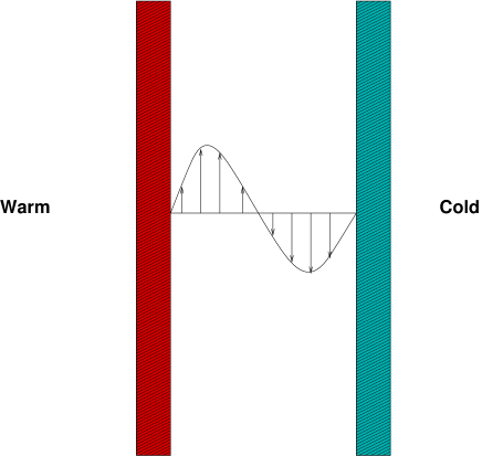
Figure 2: Flow between two vertical plates at different temperatures. This picture illustrates the shear flow generated by the baroclinic torque.

This is a vortical shear flow where vorticity is generated by the torque and diffused to the walls by viscosity.

3.2.2 Thermal wind

The second example is more closely related to our astrophysical concern. It is issued from geophysics and describes the baroclinic situation that occurs in the Earth’s atmosphere where solar heating imposes a latitudinal temperature gradient; poles which are cooler than the equator may be compared to the cold pane of the foregoing example. If the Earth were not rotating the baroclinic torque would induce, like above, a circulation between poles and equator. However, Earth rotates and therefore air cannot move easily from pole to equator because of angular momentum conservation. In this case the baroclinic torque induces an azimuthal flow; the mechanism is just similar to the one of a precessing spinner: the torque induced by the gravitationnal field on the spinner induces an azimuthal motion, namely the precession.

Let’s have a look to the equation of the flow using the Boussinesq approximation; the steady linearized inviscid momentum equation reads:

$$2\vec{\Omega}\wedge\vec{v}=-\frac{1}{\rho_{0}}{\rm NewA}\delta P-\alpha\delta T\vec{g}$$

where we neglected viscous force and non-linear terms. Here the baroclinic torque is balanced by the torque issued from Coriolis acceleration, namely

$$\mathop{\hbox{$\overrightarrow{\displaystyle\rm Rot}$}}\nolimits(2\vec{\Omega}\wedge\vec{v})=\mathop{\hbox{$\overrightarrow{\displaystyle\rm Rot}$}}\nolimits(\alpha g\delta T\vec{e}_{z})$$

More explicitely, assuming that $\delta T\equiv\delta T(x)$ ($x$ being the North-South direction), we find

$$\frac{\partial v_{y}}{\partial z}\propto\delta T^{\prime}(x)$$

This equation shows the appearance of an azimuthal $v_{y}$ flow and an axial gradient of angular momentum.

Anticipating the next section, we see that the first effect of a (baroclinic) torque is, as in the precessing spinner, to change the angular momentum distribution and not to induce a meridian circulation.

4 Rotating radiative zones - 1924 – 2004 : the evolution of ideas in eighty years

4.1 von Zeipel theorem 1924

In 1924 von Zeipel addressed the question of the equilibrium of a rotating radiative zone. Basically, he considered the point of section §3.1 in the stellar context. Let us remind us his result. If we assume that a radiative rotating envelope is in hydrostatic equilibrium, then, as we showed in 3.1, isobars, isochores, isotherms are identical and therefore all thermodynamical quantities should depend only on, say, the total potential $\Phi$ (centrifugal and gravitational); if the thermal equilibrium is realized

$$\mathop{\hbox{div}}\nolimits(\chi{\rm NewA}T)+\rho\varepsilon=0\qquad{\rm or}\qquad\mathop{\hbox{div}}\nolimits(\chi(\Phi){\rm NewA}T(\Phi))+\rho\varepsilon=0$$

$$\Longleftrightarrow\qquad\chi T^{\prime}\Delta\Phi+(\chi T^{\prime})^{\prime}({\rm NewA}\Phi)^{2}+\rho\varepsilon=0$$

where $\varepsilon$ is the rate of energy generation per unit mass. Using Poisson equation for the effective potential,

$$\underbrace{\chi(\Phi)T^{\prime}(\Phi)(4\pi G\rho(\Phi)-2\Omega^{2})}_{\rm Cte}+\underbrace{(\chi(\Phi)T^{\prime}(\Phi))^{\prime}}_{\rm Cte}\underbrace{({\rm NewA}\Phi)^{2}}_{\rm not\;Cte}+\rho\varepsilon=0$$

where ${\rm NewA}\Phi$ is just the effective gravity which is not constant on an equipotential ($\vec{g}_{\rm pole}\neq\vec{g}_{\rm eq}$). With such an equation, von Zeipel correctly concluded that an equilibrium solution is possible only if $(\chi(\Phi)T^{\prime}(\Phi))^{\prime}=0$ and if

$$\varepsilon=C\left(1-\frac{\Omega^{2}}{2\pi G\rho}\right)$$

Apparently, von Zeipel was pleased with such a result. But Eddington (1925) was not, being skeptical that energy generation, presumably of microscopic origin, could follow such a law. He suggested that hydrostatic equilibrium should be abandoned and that a meridian circulation would result from the thermal imbalance, putting forward the picture that hot poles and cool equator (or vice versa) would lead to some global convection with rising material at poles and sinking one at equator (or vice versa).

Later, the solution of von Zeipel was qualified as paradoxical by Öpik (1951) because of being not physically sound. I suppose that it is since that time that von Zeipel result is also quoted as “von Zeipel paradox”. Presently however, von Zeipel paradox rather refers to the inexistence of a static radiative equilibrium in a uniformly rotating star Busse (1982), Hansen & Kawaler (1994).

4.2 The Eddington-Sweet answer to von Zeipel paradox

The ideas of Eddington and Vogt have been transformed into a model by Sweet in 1950. The reasoning is the following: since $\mathop{\hbox{div}}\nolimits(\chi{\rm NewA}T)\neq 0$ and since we are looking for a steady solution, the velocity field which appears must be such that:

$$\rho c_{v}(\vec{v}\cdot{\rm NewA}T)=\mathop{\hbox{div}}\nolimits(\chi{\rm NewA}T)$$

Assuming the thermal imbalance, $\mathop{\hbox{div}}\nolimits(\chi{\rm NewA}T)$, is given, the temperature field being almost spherically symmetric, this equation gives an expression of the radial velocity:

$$\rho c_{v}v_{r}\frac{\partial T}{\partial r}\simeq\mathop{\hbox{div}}\nolimits(\chi{\rm NewA}T)$$

while $v_{\theta}$ is obtained from mass conservation:

$$\mathop{\hbox{div}}\nolimits(\rho\vec{v})=\frac{1}{r^{2}}\frac{\partial}{\partial r}(r^{2}\rho v_{r})+\frac{1}{r\sin\theta}\frac{\partial}{\partial\theta}(\sin\theta\rho v_{\theta})$$

The problem is that such a velocity field is not produced by a force field and therefore the conservation of angular momentum is not insured since it is not a solution of the momentum equation.

Such a difficulty was already pointed out by Randers (1941) who underlined the key role of viscosity and questioned the existence of meridian currents in an inviscid star. Then, Schwarzschild (1947), Baker & Kippenhahn (1959) and Roxburgh (1964) showed more and more explicitly that some differential rotation permits the existence of (inviscid) rotating radiative zone without meridian circulation. These authors actually pointed out the existence of the thermal wind solutions.

Kippenhahn & Weigert (1990) in Stellar structure and evolution note the problem of angular momentum conservation and the existence of solutions without meridian circulation but do not show the link between the two properties.

In fact , the connection between differential rotation, viscosity and meridian circulation were explained by Busse Busse (1981, 1982) and the first self-consistent solutions (up to a turbulence model) were given in a seminal paper by Zahn (1992).

We need now to review these two landmarks of the subject.

4.3 Busse 1981 : “Do Eddington-Sweet circulation exist?”

The problem faced by von Zeipel was presented in terms of a thermal imbalance which, through buoyancy (hot poles and cold equator), would drive a meridian circulation. However, such a steady motion is impossible in a rotating fluid because the angular momentum is not locally conserved: the flux of angular momentum induced by the meridian circulation need to be compensated by another flux (through magnetic or viscous forces for instance).

Such steady motion are thus impeded mechanically if we ignore all other forces than buoyancy. Another possibility is of course to relax the steadiness hypothesis; however, in such a case conservation of angular momentum appears as a restoring force (namely Coriolis force) which will transform any initial perturbation into a (inertial) wave motion whose transport properties are another story.

However, if the situation is stuck mechanically, it can evolve thermally. This is what occurs indeed. In this way the fluid may move… This remark underlines the real nature of the problem as it has be enounced: this is an initial value problem; then, if the time scale of the transient is short enough the star reaches a steady state or, if it is too long, initial conditions should be of dramatic influence.

To illustrate the foregoing discussion, we shall follow the work of Busse (1981) and his example in cartesian geometry. With such a set-up, one can consider arbitrary initial conditions and compute the flow and its time scales in every detail.

Busse considered a fluid with very small Prandtl number (as expected in a radiative stellar envelope) so that viscosity can be neglected in the first instance. Thus, the only source of (long term) evolution is thermal diffusion which damps out the transients to the steady state. According to our foregoing remarks which pointed the impossibility of steady meridian circulation without viscosity or magnetic field, we expect that such meridian flow occurs only during the transient.

Figure 3: Thermal wind in the cartesian analog of rotating radiative envelope.

The configuration is shown in figure 3; to keep things as simple as possible Busse considers an axisymmetric flow whose cartesian analog is:

$$\vec{v}=\left\{v(x,z)\vec{e}_{y}+\mathop{\hbox{$\overrightarrow{\displaystyle\rm Rot}$}}\nolimits(\Psi(x,z)\vec{e}_{y})\right\}e^{\lambda t}$$

where $\lambda=-\sigma+i\omega$; considering the flow is of small amplitude all nonlinear terms are neglected; the equation are further simplified by using the Boussinesq approximation. Although the system seems to be much simpler than real stars, the heart of the problem, as discovered by von Zeipel, is conserved. Baroclinicity, as it is called, is still there. Casting the equations of motions into a single scalar equation yields:

$$\left[(\omega^{2}+2i\omega\sigma)\Delta-4\Omega^{2}\frac{\partial^{2}}{\partial z^{2}}-N^{2}\frac{\partial^{2}}{\partial x^{2}}\left(1-\frac{i\kappa}{\omega}\Delta\right)\right]\Psi=0$$

which can be solved by Fourier expansions in the horizontal direction. Solutions are split into different sets of damped modes. The main ones are the gravito-inertial modes:

$$\Psi = \cos(mkx)\sin\left(n\pi(z/d+1/2)\right)$$

$$V = \frac{2\Omega n\pi}{i\omega}\cos(mkx)\cos\left(n\pi(z/d+1/2)\right)$$

$$\theta = \frac{\beta mk}{i\omega\rho_{0}}\sin(mkx)\sin\left(n\pi(z/d+1/2)\right)$$

$$\omega^{2} = \frac{4\Omega^{2}n^{2}+N^{2}(mkd/\pi)}{n^{2}+(kd/\pi)^{2}}$$

$$\sigma = \kappa k^{2}m^{2}\frac{N^{2}}{2\omega^{2}}$$

and the baroclinic modes:

$$\theta = \sin(mkx)\sin\left(n\pi(z/d+1/2)\right)$$

$$V = \frac{mk\rho\alpha gd}{2\Omega k\pi}\cos(mkx)\cos\left(n\pi(z/d+1/2)\right)$$

$$\Psi = {\cal O}(\kappa/d^{2})$$

$$\omega^{2} = 0$$

$$\sigma = \frac{\kappa}{d^{2}}\;\;\frac{n^{2}\pi^{2}+m^{2}k^{2}}{1+{N^{2}}/{4\Omega^{2}}\left({mk}/{n\pi}\right)^{2}}$$

These sets of modes should be completed by the geostrophic modes and pure thermal modes.

The fact that the Fourier basis is complete implies the completeness of the set of modes and therefore the possibility of decomposing any initial condition into a linear combination of the modes. Thus the time scale of the transient is controled by the least-damped modes. To obtain the corresponding spherical analog of this model we should make the correspondance

$$d\sim R,\qquad k\sim 2/R$$

Two damping rates associated with the two (main) sets of modes appear

$$\sigma_{GI}\sim\frac{4\kappa}{R^{2}},\qquad\sigma_{\rm baro}\sim\frac{(\pi^{2}+4)\pi^{2}}{4}\eta\frac{\kappa}{R^{2}}$$ (6)

where $\eta=\frac{4\Omega^{2}}{N^{2}}<1$. Thus we find two time scales:

• $T_{KH}=\frac{R^{2}}{\kappa}\equiv$ The thermal diffusion time or Kelvin-Helmoltz time scale

• $T_{ED}=T_{KH}/\eta\equiv$ The Eddington-Sweet time scale.

For rapid rotators $\eta\sim 1$ and all transient are damped on the Kelvin-Helmoltz time, while for slow rotators $\eta\ll 1$ baroclinic modes decay very slowly and initial conditions play a crucial role.

What about meridian circulation ? In this model it appears through $\Psi$. We see that there is some amplitude associated with gravito-inertial modes, but this is oscillatory motion which disappears after some diffusion time. Rather, the decay of baroclinic modes, which are characterized by no oscillation may be considered closer to what was imagined by Eddington, Vogt and Sweet. However, we see that either the star is rapidly rotating and such flows disappears on a Kelvin-Helmoltz time or it is slowly rotating and it keeps a strong memory of the initial conditions.

Finally, to make the discussion complete, Busse considered the Ekman layers which, through Ekman (viscous) pumping, can induce some circulation, but considering the small value of viscosity, such flows turn out to be even weaker. His paper ends with a discussion of the stability of the steady flow (the thermal wind), a stability which depends on the amplitude of course. The scenario proposed by Busse may be illustrated as in figure 4.

Back to the title of Busse’s paper “Do Eddington-Sweet circulations exist?” we clearly see that the answer is negative. In a following paper Busse (1982) aimed at popularizing this idea, Busse hammers it in: “… there are no special limits in which the Eddington-Sweet theory provides a correct solution of the basic equations”. This strong conclusion comes after forty years (since the work of Randers) during which the main stream literature has been forgetting basic physics principles !

In fact, the work of Sweet correctly derived the now well-known ’Eddington-Sweet’ time scale, which is the time it takes for the longest transient to be damped out. After Sweet (1950), this time scale is also understood as the time it takes for a fluid element to cross a distance like the radius of the star; we shall see below (§4.6) that this can be true only in an unrealistic case.

Figure 4: Busse scenario; see comments in fig. 5.

The work of Busse however considers an idealized situation where the transport coefficient are of molecular or radiative origin. Hence, the Prandtl number is very small. Actually, even a radiative zone may be the seat of some turbulence generated by (non-axisymmetric) baroclinic instabilities. Indeed, the thermal wind is basically a shear flow prone to shear instabilities. We thus expect that some turbulence takes place and enhances strongly the diffusion of momentum in stellar plasma.

But, as we pointed out, the presence of viscosity (or any local diffusive transport) changes much the situation since it permits the existence of a steady meridian circulation. We shall now examine this question through the work of Zahn (1992).

4.4 Zahn 1992

The work of Zahn (1992) is basically the implementation of Busse’s approach in the framework of spherically symmetric stars but taking into account turbulent viscosity.

The main idea is to assume that, thanks to the stable radial stratification of a radiative zone, turbulence is essentially horizontal. Hence, turbulent diffusion is strongly anisotropic, being most vigorous in the horizontal direction, implying a differential rotation developed preferentially in the radial direction.

The model concentrates on three equations:

• The advection-diffusion balance of the angular momentum flux:

  $$\frac{1}{5r^{2}}\frac{\partial}{\partial r}(\rho r^{4}U\Omega)+\frac{1}{r^{2}}\frac{\partial}{\partial r}\left(r^{4}\nu_{h}\frac{\partial\Omega}{\partial r}\right)=0$$

  where $v_{r}=U(r)P_{2}(\cos\theta)$; this form of the velocity field retains only the first term in a Legendre polynomial expansion.

• The balance of torques, source of the thermal wind,

  $$-\frac{{\rm NewA}\rho\wedge{\rm NewA}P}{\rho^{2}}={\rm NewA}\Omega^{2}\wedge s\vec{e}_{s}$$

• The advection-diffusion balance of the thermal flux

  $$\mathop{\hbox{div}}\nolimits(\chi{\rm NewA}T)+\rho\varepsilon=\rho c_{v}\vec{v}\cdot{\rm NewA}T$$ (7)

These equations are of course completed by the equation of mass conservation.

Zahn then imposes an important massage to the equation of energy (7) in order to obtain the expression of the thermal imbalance $\mathop{\hbox{div}}\nolimits(\chi{\rm NewA}T)+\rho\varepsilon$ in terms of its barotropic and baroclinic components. Each of these components are, like the velocity field, expanded onto Legendre polynomials and only the $P_{2}(\cos\theta)$-component is retained; the thermal imbalance is thus written:

$$\mathop{\hbox{div}}\nolimits(\chi{\rm NewA}T)+\rho\varepsilon=\overline{\rho}\frac{L}{M}(E_{\Omega}+E_{\mu})P_{2}(\cos\theta)$$

where $E_{\Omega}$ and $E_{\mu}$ are non-dimensional functions of rotation and compositional gradient respectively.

In section §3.5 of the paper Zahn discusses the case of the meridian velocity since its expression is easily derived from (7). There, he shows how to recover the expressions formely derived by Gratton (1945), Sweet (1950), Öpik (1951), Mestel (1966) when the rotation is assumed uniform. Of course such a rotation cannot exist by itself and need to be imposed by some trick (a magnetic field for instance although in such a case even the circulation might be suppressed, see a discussion of the case of magnetic stars in Mestel (2003)). However, as shown by Busse, if the trick is removed, these expression of the meridian circulation are pure non-sense. Indeed, a state of rigid rotation is never reach and terms coming from the $\Omega$-gradients will just cancel the $E_{\Omega}$ term ! In a steady state, radial velocity vanishes if there is no viscosity. The casual reader should therefore not overlook section §4.1 of Zahn’s paper where the dependence between circulation, viscosity and differential rotation is given explicitly (see equation 4.6). This point is emphasized in Maeder & Zahn (1998): “… not only $E_{\mu}$ but also $E_{\Omega}$ evolves to stop the circulation in a star which does not lose angular momentum”.

Figure 5: Zahn’s approach. This is the same as Busse’s one but put in another ordre. Each arrow symbolises an equation; therefore their orientation has no meaning and could be reversed! however, it is often seen in the literature that thermal imbalance implies meridian circulation. Such a statement is pure non-sense if isolated from the others; we have seen that it would be much better to say that “differential rotation implies, through viscosity, meridian circulation”. In fact, this diagram just shows that we face a system of coupled partial differential equations.

4.5 A further example

In order to further illustrate the relations between circulation, viscosity and differential rotation, we shall focus on another simple model, in the style of Busse’s but which retains viscosity and spherical geometry.

The set-up is that of a rotating, self-gravitating, full fluid sphere of nearly constant density so as to be allowed to use the Boussinesq approximation. The boundaries of the domain remain spherical whatever the rotation speed.

Within such a set-up, fluid motion, in the rotating frame, is governed by the following equations:

$$2\vec{\Omega}\wedge\vec{v}+\vec{v}\cdot{\rm NewA}\vec{v} = -\frac{1}{\rho}{\rm NewA}\delta P+\frac{\delta\rho}{\rho}(\vec{g}+\Omega^{2}s\vec{e}_{s})+\nu\Delta\vec{v}$$

$$\vec{v}\cdot{\rm NewA}\delta T = \kappa\Delta\delta T+Q$$

$$\mathop{\hbox{div}}\nolimits\vec{v} = 0$$

$$\frac{\delta\rho}{\rho} = -\alpha\delta T$$

where $\vec{v}$ is the velocity field, $\vec{\Omega}=\Omega\vec{e}_{z}$ the angular rotation of the frame, $\vec{g}$ the local gravity, $\nu$ the kinematic viscosity, $\kappa$ the thermal diffusivity, $\alpha$ the thermal dilation coefficient.

Using $R$, the radius of the sphere, as the length scale, $(2\Omega)^{-1}$ as the time scale, $T_{*}$ as the temperature scale, the non-dimensional form of the equation is:

$$\left\{\begin{array}[]{l}\vec{e}_{z}\wedge\vec{u}+\vec{u}\cdot{\rm NewA}\vec{u}=-{\rm NewA}p-\mbox{${\rm Ra}$}\Theta(-r\vec{e}_{r}+\varepsilon s\vec{e}_{s})+E\Delta\vec{u}\\ \vec{u}\cdot{\rm NewA}\Theta=E_{T}\Delta\Theta+q\\ \mathop{\hbox{div}}\nolimits\vec{u}=0\end{array}\right.$$ (8)

with the non-dimensional numbers

$$\mbox{${\rm Ra}$}=\frac{\alpha T_{*}g}{4\Omega^{2}R},\qquad\varepsilon=\frac{\Omega^{2}R}{g}$$

which control the driving and the other numbers

$$E=\frac{\nu}{2\Omega R^{2}},\qquad E_{T}=\frac{\kappa}{2\Omega R^{2}},$$

which control the diffusion.

The system (8) is simplified by elimination of the barotropic component of the background which is spherically symmetric and in hydrostatic equilibrium; we thus write:

$$\vec{u}=\varepsilon\vec{u}_{1},\qquad\Theta=\Theta_{0}(r)+\varepsilon\Theta_{1},\qquad p=p_{0}(r)+\varepsilon p_{1}$$

Furthermore, if we introduce the Brunt-Väisälä  frequency

$$N^{2}_{T}=\alpha\frac{dT_{0}}{dr}g=4\Omega^{2}\mbox{${\rm Ra}$}r\Theta^{\prime}_{0}(r)$$

and set $\mbox{${\rm Ra}$}\,r\Theta^{\prime}_{0}=rn^{2}(r)$, the equation of motion may be cast into:

$$\left\{\begin{array}[]{l}\mathop{\hbox{$\overrightarrow{\displaystyle\rm Rot}$}}\nolimits\left[\vec{e}_{z}\wedge\vec{u}+\varepsilon\vec{u}\cdot{\rm NewA}\vec{u}-(r\vec{e}_{r}-\varepsilon s\vec{e}_{s})\Theta_{1}-E\Delta\vec{u}\right]=-rn^{2}\sin\theta\cos\theta\vec{e}_{\varphi}\\ \\ n^{2}u_{r}+\varepsilon\vec{u}\cdot{\rm NewA}\Theta_{1}=E_{T}\Delta\Theta_{1}\\ \\ \mathop{\hbox{div}}\nolimits\vec{u}=0\end{array}\right.$$ (9)

The equation of vorticity clearly shows that the motion is driven by the baroclinic torque, $-rn^{2}\sin\theta\cos\theta\vec{e}_{\varphi}$ issued from the set-up. We are therefore facing the problem of a steady forced flow. We may further simplify the problem by considering small $\varepsilon$, i.e. small centrifugal effect; at first order the flow is controlled by the linear equations:

$$\left\{\begin{array}[]{l}\mathop{\hbox{$\overrightarrow{\displaystyle\rm Rot}$}}\nolimits\left(\vec{e}_{z}\wedge\vec{u}-r\vec{e}_{r}\Theta_{1}-E\Delta\vec{u}\right)=-rn^{2}\sin\theta\cos\theta\vec{e}_{\varphi}\\ \\ n^{2}u_{r}=E_{T}\Delta\Theta_{1}\\ \\ \mathop{\hbox{div}}\nolimits\vec{u}=0\end{array}\right.$$ (10)

It is quite easy to see that if viscosity is neglected, the thermal wind

$$\left\{\begin{array}[]{l}\vec{u}=\left(-s\int n^{2}(r)dr+F(s)\right)\vec{e}_{\varphi},\\ \\ \Theta_{1}=0\end{array}\right.$$ (11)

is a solution of the equations. Here $s=r\sin\theta$ is the radial cylindrical coordinate and $F(s)$ an arbitrary function describing a pure geostrophic solution. We thus find again that in such a baroclinic steady flow, no meridian circulation is allowed if viscosity is zero.

The dependance between viscosity and meridian circulation may be made even more explicit if we project the system (10) on the spherical harmonics and have a look to first terms. Following Rieutord (1987), we set

$$\vec{u}=\sum_{l=0}^{+\infty}\sum_{m=-l}^{+l}u^{\ell}_{m}\vec{R}^{m}_{\ell}+v^{\ell}_{m}\vec{S}^{m}_{\ell}+w^{\ell}_{m}\vec{T}^{m}_{\ell},\qquad\Theta_{1}=\sum_{l=0}^{+\infty}\sum_{m=-l}^{+l}\theta^{\ell}_{m}Y^{m}_{\ell}$$

where

$$\vec{R}^{m}_{\ell}=Y^{m}_{\ell}\vec{e}_{r},\qquad\vec{S}^{m}_{\ell}={\rm NewA}Y^{m}_{\ell},\qquad\vec{T}^{m}_{\ell}={\rm NewA}\times\vec{R}^{m}_{\ell}$$

with $Y^{m}_{\ell}$ being the usual normalized spherical harmonic function. The projection of the equation leads to

$$\left\{\begin{array}[]{l}E\Delta_{l}w^{l}_{m}+A^{l}_{l-1}r^{l-1}\frac{\partial}{\partial r}\biggl{(}\frac{u_{m}^{l-1}}{r^{l-2}}\biggr{)}+A^{l}_{l+1}r^{-l-2}\frac{\partial}{\partial r}\biggl{(}r^{l+3}u_{m}^{l+1}\biggr{)}=0\\ \\ E\Delta_{l}\Delta_{l}(ru^{l}_{m})=B^{l}_{l-1}r^{l-1}\frac{\partial}{\partial r}\biggl{(}\frac{w_{m}^{l-1}}{r^{l-1}}\biggr{)}+B^{l}_{l+1}r^{-l-2}\frac{\partial}{\partial r}\biggl{(}r^{l+2}w_{m}^{l+1}\biggr{)}\\ \qquad\qquad\qquad\qquad+l(l+1)\theta^{l}_{m}-6rn^{2}(r)N_{2}\delta_{l2}\\ \\ E_{T}\Delta_{\ell}\theta^{l}_{m}-n^{2}(r)u^{l}_{m}=0\\ \end{array}\right.$$

where $N_{2}=\frac{1}{6}\sqrt{\frac{16\pi}{5}}$ and $A^{l}_{l-1},B^{l}_{l-1},...$ are coupling coefficients. This is the set of ordinary differential equations which can be solved numerically to obtain the full solution. However, for the pedagogical matters we are interested in, it is sufficient to consider $\ell\leq 2$. We thus have:

$$\left\{\begin{array}[]{l}E\Delta_{1}w^{1}+A^{1}_{2}r^{-3}\frac{\partial}{\partial r}\biggl{(}r^{4}u^{2}\biggr{)}=0\\ \\ E\Delta_{2}\Delta_{2}(ru^{2})=B^{2}_{1}r^{1}\frac{\partial}{\partial r}\biggl{(}\frac{w^{1}}{r}\biggr{)}+6\theta^{2}-6rn^{2}N_{2}\\ \\ E_{T}\Delta_{2}\theta^{2}-n^{2}u^{2}=0\\ \end{array}\right.$$

In the axisymmetric problem which is considered here $u^{\ell}$’s represent the radial velocity and therefore meridian velocity while $w^{\ell}$’s describe the azimuthal velocity. The first equation shows that if viscosity is zero, i.e. $E=0$, then $u^{2}=0$, hence no meridian flow occurs and the temperature field is in equilibrium; the gradient of the azimuthal flow, $B^{2}_{1}r\frac{\partial}{\partial r}\biggl{(}\frac{w^{1}}{r}\biggr{)}$ just compensates the baroclinic torque $-rn^{2}6N_{2}$.

From these equations we may see that, when viscosity is taken into account, the shear drives a meridian circulation which in turns drives thermal imbalance !

4.6 Some additional remarks

The foregoing example may be completed by the work of Garaud (2002) which presents numerical solutions of the same problem but in a more realistic set-up: there, the Boussinesq approximation is relaxed; instead the anelastic approximation is used to filter out sound waves and permits the existence strong density contrasts of the background. Thus, radial profiles of pressure, temperature or density, are more stellar or solar like.

Garaud (2002) shows that steady flows are controlled by the non-dimensional ratio $\lambda={\cal P}N^{2}/\Omega^{2}={\cal P}/\eta$ (see (6) for the definition of $\eta$). For $\lambda\gg 1$, i.e. for slow rotation, it is shown that the scaling of meridian velocity is indeed that of Eddington-Sweet, this circulation is confined to a layer close to the outer boundary. In the case of a fast rotation $\lambda\ll 1$ however, Garaud finds that meridian flows scale as $\nu/r$ in agreement with our foregoing discussion.

Could it be that Sweet’s result applies to slowly rotating stars? In this case indeed the result found by Garaud gives an amplitude of the circulation which is independent of viscosity and which corresponds to a turn over time equal to the Eddington-Sweet time. Let us first note that extremely slow rotation are needed; indeed, $\lambda\gg 1$ means $\eta\ll{\cal P}$, while we know that ${\cal P}\ll 1$ in a radiative zone. Hence, this result applies only when Eddington-Sweet time is at least ${\cal P}^{-1}$ greater than thermal diffusion time (i.e. Kelvin-Helmoltz time); in such conditions, it is clear that Eddington-Sweet time is much longer than the actual lifetime of the star. Therefore, back to Busse’s result, it is also clear that such a steady state is never reached.

4.7 Unsteady situations

This discussion brings us to the question of the role of initial conditions. Until now we focused our attention to the case of steady flows, however if the star is initially rotating slowly so that Eddington-Sweet time exceeds nuclear time, it is clear that, according to Busse, the rotational state of the star will be marked by the initial conditions. In such case modeling the actual dynamical state of star requires the knowledge of an enormous number of parameters, namely the initial velocity field (at least!).

However, as shown by observations, young stars are rather rapid rotators and therefore we may expect that they reach a sort of universal state of differential rotation. But it is also well known that in the course of their lives, stars lose angular momentum and thus progressively slow down their rotation.

4.8 Spin-down processes

This remark brings us to the role of winds and angular momentum losses. As already stressed by Zahn (1992), this is certainly the main source of mixing for main sequence stars. The supposed universal differential rotation which comes out of the balance between baroclinic torque and (turbulent) viscosity is thus perturbed by the shear produced by the angular momentum loss. In fact this becomes the dominant source of turbulence in radiative zone and the dynamical state of the star is now controlled by the mechanisms which insure the angular momentum transfer between the different layers. It may be turbulent diffusion, but also gravity waves emitted by a neighbouring convective zone (see Talon & Charbonnel, 2003).

To give an intuitive idea of how a spin down process works, it is useful to go back to the laboratory. Consider a fluid contained in some rotating container; at some time when the fluid is in perfect solid rotation, the rotation of the container is slowed down by some small amount (so that all the spin-down process remains controlled by linear equations). After some rotation, Ekman boundary layers form on the wall of the container which are not parallel to the rotation axis. These layers are the seat of shear flow parallel to the wall and when the wall imposes a no-slip boundary conditions, dissipation is very intense there. However, in addition to this dissipative process, Ekman layers also pump the fluid into or out of the layer. By this process, the layer drives a circulation in the bulk of the fluid mass, thus inducing a transport of angular momentum from the bulk to the layer. In a laboratory experiment the friction of the fluid, through viscosity, on the container’s wall, finally removes the angular momentum from the fluid. The circulation, induced by the Ekman layer, plays a fundamental role in the spin-down process since it governs the time-scale of the process. This time scale is indeed

$$(2\Omega)^{-1}\left(\frac{2\Omega L^{2}}{\nu}\right)^{1/2}$$

much smaller than the diffusion time scale $L^{2}/\nu$.

Back to the case of stars there are some differences, which still need to be investigated in detail, but the gross features are certainly quite similar.

There are of course no rigid wall at the surface of a star; however, if we consider the case of a solar type star with an outer envelope threaded by magnetic fields, it is likely that the convective envelope will lose quite rapidly its angular momentum and behave like a rigid body stressing the lower radiative zone. There everything depends on the viscosity : if strong enough it can extract angular momentum at the desired rate imposed by the wind. On the contrary, the shear layers may become unstable and turbulence should develop enhancing the viscosity; the foregoing situation may be restored and extraction takes the imposed rate; however, shear has a maximum value and therefore the stress (equal to shear times viscosity) may not be high enough; in such a case, called strong wind in Zahn (1992), the radiative zone will slow down at a rate controlled by turbulent diffusive processes.

In this description we have not described the effect of stratification and heat diffusion which make the whole picture a little more complex. In fact the whole problem has been only touched upon and the whole non-linear scenario is waiting exploration. Basic references on spin-down process in the laboratory context are Greenspan (1969) or Rieutord (1997); a discussion on the effect of stratification and small Prandtl number can be found in Friedlander (1976); an application to the stellar (solar) context has been tempted by Zahn et al. (1997).

5 Summarizing essential points

To end this lecture I would like to stress the most important points, those one should keep in mind when dealing with rotating radiative zones.

First we need to stress that

$$\rho c_{v}\vec{v}\cdot{\rm NewA}T=\mathop{\hbox{div}}\nolimits(\chi{\rm NewA}T)+\varepsilon$$

is not an equation determining the velocity field. It determines the temperature once $\vec{v}$ is given by the dynamics; there is no other mean to determine the temperature. Giving an a-priori-approximate-solution for $T$ and using it to derive $\vec{v}$ is just an incorrect reasoning. Any approximate solution of $\vec{v}$ needs to be a solution of both the momentum and energy equation (or a combination of both).

It is another error to specify to rotation state (usually assumed rigid) as it will quickly (on a Kelvin-Helmoltz time however) evolve to a differential rotation state thanks to the diffusion of heat. Even if rotation is slow, such a reasoning is misleading since the rotation state at time $t$ is the result of an evolution which cannot be discarded; initial conditions, which are usually a fast and differential rotation are not forgotten by a presently slowly rotating star.

Finally, we have shown that viscosity (or any source of diffusion of momentum) plays a crucial part in the dynamical evolution of a star, in particular in mixing processes. An isolated star (no wind) cannot sustain a large-scale circulation in a quasi-steady state if no diffusion process occurs.

Finally, let us stress that the loss of angular momentum is another crucial aspect for the mixing processes since these losses also drive meridian circulation. It underlines again the importance of the dynamical history of a star when one tries to understand its present surface abundances.