A weakly nonlinear analysis of the magnetorotational instability in a model channel flow

Abstract

We show by means of a perturbative weakly nonlinear analysis that the axisymmetric magnetorotational instability (MRI) of a viscous, resistive, incompressible rotating shear flow in a thin channel gives rise to a real Ginzburg-Landau equation for the disturbance amplitude. For small magnetic Prandtl number (${\cal P}_{\rm m}$), the saturation amplitude is $\propto\sqrt{{\cal P}_{\rm m}}$ and the resulting momentum transport scales as ${\cal R}^{-1}$, where $\cal R$ is the hydrodynamic Reynolds number. Simplifying assumptions, such as linear shear base flow, mathematically expedient boundary conditions and continuous spectrum of the vertical linear modes, are used to facilitate this analysis. The asymptotic results are shown to comply with numerical calculations using a spectral code. They suggest that the transport due to the nonlinearly developed MRI may be very small in experimental setups with ${\cal P}_{\rm m}\ll 1$.

The magnetorotational instability (MRI) has acquired growing theoretical and experimental interest in recent years, moving beyond just the astrophysical community. The linear MRI has been known for almost 50 years veli ; chandra1 : Rayleigh stable rotating Couette flows of conducting fluids are destabilized in the presence of a vertical magnetic field if $d\Omega^{2}/dr<0$ (angular velocity decreasing outward). However, the MRI only acquired importance to astrophysics after the influential work of Balbus & Hawley baha1 , who demonstrated its viability to accretion disks (for any sufficiently weak field) with linear analysis supplemented by nonlinear numerical simulations. Enhanced transport (conceivably turbulent) is necessary for accretion to proceed in disks found in a variety of astrophysical settings - from protostars to active galactic nuclei. The difficulty in identifying sources of such enhanced transport has been a limitation to proper theoretical understanding and modeling of these objects. Thus the MRI has been widely accepted as an attractive solution for enhanced transport (see the comprehensive reviews rev1 ; rev2 ) even though some questions on the nature of MRI-driven turbulence remain brand . Because of the MRI’s importance and some of its outstanding unresolved issues, several groups have recently undertaken projects to investigate the instability under laboratory conditions jgk ; colgate ; sisan . Additionally, numerical simulations specially designed for experimental setups have been conducted.

In this Letter we perform a weakly nonlinear analysis of the MRI near threshold for a rotating flow in channel geometry, subject to idealized but mathematically expedient boundary conditions. This kind of approach is important because the viability of this linear instability as the driver of turbulence and angular-momentum transport relies on understanding its nonlinear development and saturation. By complementing the above mentioned simulations, analytical methods remain useful to gain further physical insight. To facilitate an analytical approach we make a number of simplifying assumptions so as to make the system amenable to well-known methods BO ; crossandI ; manbook ; mybook for the derivation of nonlinear envelope equations (i.e. with an amplitude weakly dependent on time and space). Additionally we assume a narrow channel geometry, i.e. the small-gap limit of Taylor-Couette flow.

The hydromagnetic equations in cylindrical coordinates chandra are applied to the neighborhood of a representative point in the system, using the shearing box (SB) approximation goldreich65 . The SB has been employed in numerous (analytical and numerical) studies of the MRI in accretion disks and are also appropriate for this model problem. Within the framework of the small shearing box (SSB)SSB , the base flow is steady and incompressible with constant pressure. The velocity ${\bf V}=U(x){\bf{\hat{y}}}$ has a linear shear profile $U(x)=-qU_{0}x$, representing an axisymmetric flow about a point $r_{0}$, that rotates with a rate $\Omega_{0}$ defined from the differential rotation law $\Omega(r)\propto\Omega_{0}(r/r_{0})^{-q}$. We restrict ourselves to a constant initial magnetic field ${\bf B}=B_{0}{\bf\hat{z}}$. Cartesian coordinates $x,y,z$ are used to represent the radial (shear-wise), azimuthal (stream-wise) and vertical directions, respectively. The base flow is axisymmetricaly disturbed by perturbations of the velocity, ${\bf u}=(u_{x},u_{y},u_{z})$, magnetic field, ${\bf b}=(b_{x},b_{y},b_{z})$, and total pressure, $\varpi$. This results, after non-dimensionalization, in the following set of non-linear equations:

$$\frac{d{\bf u}}{dt}-2{{\bf{\hat{z}}}\times{\bf u}}-{qu_{x}{\bf{\hat{y}}}}-{\cal C}\,\hat{\mathbb{B}}\,{\bf b}=-\nabla\varpi+\frac{1}{{\cal R}}\nabla^{2}{\bf u}\ \ \ \ \$$ (1a)

$$\frac{d{\bf b}}{dt}-\hat{\mathbb{B}}\,{\bf u}+{qb_{x}{\bf{\hat{y}}}}=\frac{1}{{\cal R}_{{\rm m}}}\nabla^{2}{\bf b}$$ (1b)

$$\nabla\cdot{\bf u}=0~{}~{}~{}~{}{\rm and}~{}~{}~{}~{}\nabla\cdot{\bf b}=0,$$ (1c)

where $\hat{\mathbb{B}}\equiv({\bf b}\cdot\nabla+B_{0}\partial_{z})$. Lengths were scaled by $\tilde{L}$ (the channel width scale), time by $\tilde{\Omega}_{0}^{-1}\equiv\Omega_{0}^{-1}$ and the magnetic field by $\tilde{B}_{0}\equiv B_{0}$. The quantities marked by tilde are thus dimensional. With this scaling, $B_{0}=1$ in (1) but we retain it for later convenience. The non-dimensional parameter ${\cal C}\equiv\tilde{B}_{0}^{2}/(4\pi\tilde{\rho}_{0}\tilde{\Omega}^{2}\tilde{L}^{2})\equiv\tilde{V}_{A}^{2}/\tilde{U}^{2},$ is the Cowling number, measuring the dynamical importance of the magnetic field. In addition the Reynolds number, ${\cal R}\equiv\tilde{\Omega}_{0}\tilde{L}^{2}/\tilde{\nu},$ and the magnetic Reynolds number, ${\cal R}_{\rm m}\equiv\tilde{\Omega}_{0}\tilde{L}^{2}/\tilde{\eta},$ are used, where $\tilde{\nu}$ and $\tilde{\eta}$ are the microscopic kinematic viscosity and magnetic resistivity of the fluid, respectively. We introduce two additional non-dimensional parameters, which figure in what follows: the Elsasser number, ${\cal S}\equiv{\cal R}_{\rm m}{\cal C}=\tilde{B}_{0}^{2}/(4\pi\tilde{\rho}_{0}\tilde{\Omega}_{0}\tilde{\eta}),$ and the magnetic Prandtl number, ${\cal P}_{\rm m}\equiv{\cal R}_{\rm m}/{\cal R}$.

Linearization of (1), for perturbations of the form $\propto e^{st+ik_{x}x+ik_{z}z}$, gives rise to the dispersion relation,

$$a_{0}s^{4}+a_{1}s^{3}+a_{2}s^{2}+a_{3}s+a_{4}=0,$$

where all the $a_{i}=a_{i}(k_{x},k_{z},{\cal P}_{\rm m},{\cal S},{\cal C},q)$ but we shall write explicitly only $a_{4}$:

$$\frac{{\cal C}}{{\cal S}^{4}}\Bigl{[}k_{{}_{T}}^{2}{\cal C}({\cal C}k_{{}_{T}}^{4}{\cal P}_{\rm m}+k_{z}^{2}{\cal S}^{2})^{2}+\kappa^{2}{\cal S}^{2}{\cal C}k_{{}_{T}}^{4}k_{z}^{2}-2q{\cal S}^{4}k_{z}^{4}\Bigr{]},$$ (2)

where the notation $\kappa^{2}\equiv 2(2-q),\ k_{{}_{T}}^{2}\equiv k_{x}^{2}+k_{z}^{2}$ is introduced.

For given values of the parameters (we denote them collectively as $\Pi$) there will be four distinct modes. The linear theory in various limits for this problem has been discussed in numerous publications (see rev1 ; rev2 ) and we shall not elaborate upon them any further. Rather, we focus on situations where the most unstable mode (of the four) is marginal (critical) for some $k_{z}$ at a given value of $k_{x}=K$. We fix $K$ in order to focus on the marginal vertical dynamics within a channel (see below).

Marginality to the MRI ($s=0$) implies the vanishing of the real coefficient $a_{4}$ (as expressed above) and its derivative with respect to $k_{z}$ at some $k_{z}=Q$:

$$a_{4}(k_{z}=Q;K,\Pi)=0,\ \ \frac{\partial a_{4}}{\partial k_{z}}(k_{z}=Q;K,\Pi)=0.$$ (3)

The second condition and (2) yield

$$Q\Bigl{[}Q^{2}{\cal S}^{4}({\cal C}Q^{2}-4q)+(K^{2}+Q^{2})2Q^{2}{\cal C}{\cal S}^{2}({\cal S}^{2}+\kappa^{2})$$

$$+(K^{2}+Q^{2})^{2}{\cal C}{\cal S}^{2}(6{\cal C}{\cal P_{\rm m}}Q^{2}+\kappa^{2})+2(K^{2}+Q^{2})^{3}{\cal P_{\rm m}}{\cal C}^{2}{\cal S}^{2}$$

$$+5(K^{2}+Q^{2})^{4}{\cal P_{\rm m}}^{2}{\cal C}^{3}\Bigl{]}=0.$$ (4)

This equation, together with $a_{4}(k_{z}=Q,K;\Pi)=0$, can be solved for ${\cal S}$ and $Q$. The general expressions for ${\cal S}(K,{\cal P}_{\rm m},{\cal C},q)$ and $Q(K,{\cal P}_{\rm m},{\cal C},q)$ are lengthy but their asymptotic forms, for ${\cal P}_{\rm m}\ll 1$, to leading order,

$${\cal S}=\frac{\sqrt{16\ {\cal C}q(2-q)}K}{(2q-{\cal C}K^{2})},\ \ Q^{2}=K^{2}\frac{2q-{\cal C}K^{2}}{2q+{\cal C}K^{2}}.$$ (5)

If ${\cal C}K^{2}>2q$ the solutions are not physically meaningful, while the case ${\cal C}K^{2}=2q$ corresponds to the ideal MRI limit.

We consider the properties of the MRI within the confines of an idealized model channel geometry with walls located at $x=0,\pi/K$. We allow all quantities to be vertically periodic on a scale $L_{z}$ commensurate with integer multiples of $2\pi/Q$. As long as $L_{z}\gg 1/Q$, the limit of a vertically extended system (and thus a continuous spectrum of vertical modes) may be affected.

We follow the fluid into instability by tuning the vertical background field away from the steady state, i.e. $B_{0}\rightarrow 1-\epsilon^{2}\tilde{\lambda},$ where $\epsilon\ll 1$ and $\tilde{\lambda}$ is an ${\cal O}\left({1}\right)$ control parameter. This means that we are now in a position to apply procedures of singular perturbation theory to this problem, by employing the multiple-scale (in $z$ and $t$) method (e.g, BO ). It facilitates, by imposing suitable solvability conditions at each expansion order of the calculation in order to prevent a breakdown in the solutions, a derivation of an envelope equation for the unstable mode. Thus for any dependent fluid quantity $F(x,z,t)$ we assume

$$F(x,z,t)=\sum_{i=1}^{\infty}\epsilon^{i}F_{i}(x,z,t).$$ (6)

The fact that the $x$ and $z$ components of the velocity and magnetic field perturbations can be derived from a streamfunction, $\Psi(x,z)$ and magnetic flux function $\Phi(x,z)$ reduces the number of relevant dependent variables $F$ to four ($u_{y}$ and $b_{y}$ are the additional two). These four dependent variables will also be used in the spectral numerical calculation (see below).

For the lowest $\epsilon$ order of the equations, resulting from substituting the expansions into the original PDE and collecting same order terms, we make the Ansatz $F_{1}(x,z,t)=\hat{F}_{1}\tilde{A}(\epsilon z,\epsilon^{2}t)e^{iQz}\sin Kx+{\rm c.c.},$ where $\hat{F}_{1}$ is a constant (according to the variable in question), and where the envelope function $\tilde{A}$ (an arbitrary constant amplitude in linear theory) is now allowed to have weak space (on scale $Z\equiv\epsilon z$) and time (on scale $T\equiv\epsilon^{2}t$) dependencies. Because this system is tenth order in $x$-derivatives, a sufficient number of conditions must be specified at the edges. The $\sin Kx$ functional dependence of the Ansatz satisfies the ten boundary conditions

$$u_{x}=u_{y}=b_{x}=b_{y}=\partial_{x}u_{z}=0,$$ (7)

at $x=0,\pi/K$. These conditions are also subsequently satisfied to all orders of the expansion procedure because of the symmetry property of $\sin Kx$ under the nonlinear operations of (1). These specifications are a mixture of kinematic conditions on the edges: no-slip conditions on $u_{x}$ and $u_{y}$ with free-slip conditions on $u_{z}$. The conditions are similarly mixed for the magnetic field: conducting conditions on $b_{x}$ and insulating conditions on $b_{y}$. Although these conditions are idealized, they are mathematically expedient, in that the coefficients of the resulting envelope equation may be expressed analytically in the limit ${\cal P}_{\rm m}\ll 1$, and they serve to capture the salient features of the resulting dynamics (see below).

The end result of the asymptotic procedure procedure is the well-known real Ginzburg-Landau Equation (GLE) which, for ${\cal P}_{\rm m}\ll 1$, is

$$\partial_{T}A=\lambda A-\frac{1}{{\cal P}_{\rm m}{\cal C}}A|A|^{2}+D\partial_{{}_{Z}}^{2}A.$$ (8)

Here $A\equiv{\sqrt{\xi}}\tilde{A}$, $\lambda\equiv\zeta\tilde{\lambda}$, and the coefficients, for a value of $q=3/2$ (corresponding to a Keplerian shear flow) are

$$\xi = \frac{3}{4}\cdot\frac{5{\cal S}^{4}-18{\cal S}^{2}-32+2({\cal S}^{2}+16)\sqrt{{\cal S}^{2}+1}}{{\cal S}({\cal S}^{2}+1)(4\sqrt{{\cal S}^{2}+1}-3)},\ \ \$$ (9a)

$$D = 6\frac{\left({\cal S}^{2}+2-2\sqrt{{\cal S}^{2}+1}\right)({\cal S}^{2}+1)}{{\cal S}^{3}(4\sqrt{{\cal S}^{2}+1}-3)},$$ (9b)

$$\zeta = \frac{3{\cal S}\sqrt{{\cal S}^{2}+1}-6{\cal S}}{4{\cal S}^{2}+1+\sqrt{{\cal S}^{2}+1}},$$ (9c)

where ${\cal S}(K)$ is as given in (5). The expressions for a general $q$ are very long and involved. For ${\cal S}\gg 1$, (i.e. as one approaches the ideal MRI limit), these simplify to $\xi=15/16,\ \zeta=3/4,\ D=3/2$; and in general they remain ${\cal O}\left({1}\right)$ quantities for all reasonable values of ${\cal S}$.

Before proceeding any further, it is important to note that equations (1) admit an integral relationship for the total disturbance energy. Application of the boundary conditions (7) yields a hydromagnetic extension of the Reynolds-Orr equation sh . Here it takes on the form:

$$\frac{d{\rm E}_{\rm V}}{dt} = -\frac{dU}{dx}\int(u_{x}u_{y}-{\cal C}b_{x}b_{y})dxdz$$ (10)

$$-\int{\left(\frac{1}{{\cal R}}|\nabla{\bf u}|^{2}+\frac{1}{\cal R_{{\rm m}}}{\cal C}|\nabla{\bf b}|^{2}\right)dxdz},\ \ \ \ \$$

where $|\nabla{\bf u}|^{2}\equiv\sum_{\mu}|\nabla u_{\mu}|^{2}$ for $\mu=x,y,z$ and similarly for ${\bf b}$. ${\rm E}_{\rm V}$ is the total energy, per unit length in the azimuthal direction, of the disturbances in the domain, ${\rm E}_{\rm V}\equiv\mbox{$\frac{1}{2}$}\int{\left({\bf u}^{2}+{\cal C}{\bf b}^{2}\right)dxdz}$, and the first integral (multiplied by $dU/dx$) represents the energy fed into the hydrodynamical and magnetic disturbances by the background shear. The integrand ${\rm T}\equiv u_{x}u_{y}-{\cal C}b_{x}b_{y}$ is the relevant component of the total stress in the disturbance. Integrating it along the wall and averaging radially gives an estimate of the average angular momentum transport rate inside the channel, i.e. ${\rm{\dot{J}}}\equiv(K/\pi)\int_{-L_{z}/2}^{L_{z}/2}\int_{0}^{\pi/K}{{\rm T}dxdz}$.

We can use our asymptotic solutions to express ${\rm E_{\rm V}}$ and $\dot{\rm J}$ in terms of the envelope function $A(Z,T)$. To the first few leading orders in $\epsilon$ (recalling that ${\cal P}_{\rm m}\ll 1$) we find that

$${\rm E}_{\rm V}=\epsilon^{2}\alpha({\cal S}){\cal C}^{2}A^{2}+\epsilon^{4}{\cal C}^{3}\left[\frac{\beta_{2}({\cal S})}{{\cal P}_{\rm m}^{2}}+\frac{\beta_{1}({\cal S})}{{\cal P}_{\rm m}}\right]A^{4}+\cdots.$$

$\alpha$ and $\beta_{i}$ are functions whose value is of ${\cal O}\left({1}\right)$ for all reasonable values of ${\cal S}(K,q=3/2)$. The two bracketed terms arise from the second order (in $\epsilon$) azimuthal velocity disturbances. Contributions to the total angular momentum transport ($\dot{\rm J}=\dot{\rm J}_{\rm H}+\dot{\rm J}_{\rm B}$) due to the hydrodynamic ($\dot{\rm J}_{\rm H}$) and magnetic correlations ($\dot{\rm J}_{\rm B}$) are, to leading order,

$$\dot{\rm J}_{\rm H} = \frac{9\epsilon^{2}}{{\cal S}}\left(\frac{2+{\cal S}^{2}-2\sqrt{1+{\cal S}^{2}}}{1+{\cal S}^{2}}\right)A^{2}+{\cal O}\left({\epsilon^{3},\epsilon^{2}{\cal P}_{\rm m}}\right),\ \ \ \ \$$ (11a)

$$\dot{\rm J}_{\rm B} = \frac{3\epsilon^{2}}{{\cal S}}\left(1-\frac{1}{\sqrt{1+{\cal S}^{2}}}\right)A^{2}+{\cal O}\left({\epsilon^{3},\epsilon^{2}{\cal P}_{\rm m}}\right).$$ (11b)

The envelope $A$ is found by solving the GLE, which is a well-studied system (see, e.g., mybook for a summary and references). It has three steady uniform solutions in one spatial dimension (here, the vertical): an unstable state $A=0$, and two stable states $A=\pm A_{s}$, where $A_{s}^{2}=|\zeta({\cal S})|{\cal P}_{\rm m}{\cal C}$ (note that $\zeta({\cal S})$ is an ${\cal O}\left({1}\right)$ quantity). $A_{s}$ is also the saturation amplitude, because the system will develop towards it mybook .

Setting $A\rightarrow A_{s}$ in (11a-b) and in the expression for ${\rm E_{V}}$, followed by some algebra, reveals that the angular momentum flux in the saturated state is, to leading order in ${\cal P}_{\rm m}$ and $\epsilon$, $\dot{\rm J}=\epsilon^{2}|\zeta({\cal S})|\gamma({\cal S}){\cal P}_{\rm m}{\cal C}{\cal S}^{-1}$, while in the expression for the energy one term is independent of ${\cal P}_{\rm m}$, ${\rm E_{V}}=\epsilon^{4}{\cal C}^{3}\zeta^{2}({\cal S})\beta_{2}({\cal S})+{\cal O}\left({{\cal P}_{\rm m}}\right)$.

The key results of this idealized analysis are thus,

$$A_{s}\sim\sqrt{{\cal P}_{\rm m}{\cal C}}\longrightarrow{\rm E_{V}}\sim E_{0},~{}~{}~{}~{}\dot{\rm J}\sim{\cal R}^{-1},$$ (12)

for ${\cal P}_{\rm m}\ll 1$, where $E_{0}$ is a constant, independent of ${\cal P}_{\rm m}$.

We have also performed numerical calculations, using a 2-D spectral code to solve the original nonlinear equations (1), in the streamfunction and magnetic flux function formulation, near MRI threshold. The asymptotic theory reflects the trends seen in these simulations. The code implements a Fourier-Galerkin expansion in ${\rm 64}\times{\rm 64}$ modes in each of the four independent physical variables, i.e. ${\bf F}=\sum_{n,m}{\bf F}_{\rm nm}(t)\sin K_{n}xe^{iQ_{m}z}+{\rm c.c.}$, where ${\bf F}=(\psi,u_{y},\Phi,b_{y})^{{\rm T}}$ and where ${\bf F}_{\rm nm}(t)$ is the time-dependent amplitude of the particular Fourier-Galerkin mode in question (denoted by the indices $n,m$).

We typically start with white noise initial conditions on ${\bf F}_{\rm nm}(0)$ at a level of 0.1 the energy of the background shear. Because of space limitations we display only a representative plot of runs made with ${\cal S}=5.0$, ${\cal C}=0.05$, (i.e. ${\cal R}_{\rm m}$ fixed), $q=3/2$ and $\epsilon^{2}=0.2$ for a few successively increasing values of ${\cal R}$ (see Figure 1). Note that with this value of $\epsilon$ the fastest growing linear mode has a growth rate of $\sim 0.065$ in these units, and thus fully developed ideal MRI can not be expected.

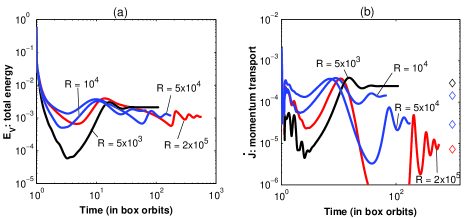
Figure 1: ${\rm E_{V}}$ (panel a) and $\dot{\rm J}$ (panel b) as a function of time from numerical calculation. The black line is for ${\cal R}=5\times 10^{3}$, the red one for ${\cal R}=2\times 10^{5}$. The intermediate values (in blue) are successively for ${\cal R}=10^{4},5\times 10^{4}$. The diamonds in panel (b) show the scaling predicted by our asymptotic analysis, which also predicts a constant final value of the disturbance energy, as apparent in panel (a). One box orbit $=2\pi$ in nondimensionalized units.

It is apparent that ${\rm E}_{\rm V}$ saturates at a constant independent of ${\cal R}$ (for large enough $\cal R$, i.e. small enough ${\cal P}_{\rm m}$), while $\dot{\rm J}$ saturates at values that scale as ${\cal R}^{-1}$, as expected from our asymptotic analysis.

The numerical and asymptotic solutions developed here show that in the saturated state the second order azimuthal velocity perturbation becomes dominant over all other quantities for ${\cal P}_{\rm m}\ll 1$: it has the spatial form $\sin 2Kx$, independent of $z$. It arises from the ${\cal O}\left({\epsilon^{2}}\right)$ term in asymptotic expansion (6), and appears to be the primary agent in the nonlinear saturation of the MRI in the channel. It acts anisotropically so as to modify the shear profile and results in a non-diagonal stress component (relevant for radial angular momentum transport), which behaves like $\sim 1/{\cal R}$.

These results should be compared to experiments and their numerical simulations. Thus far no experimental results for this geometry have been reported but corresponding numerical simulations do exist jeremy . Our results on the scaling of transport (decreasing with increasing ${\cal R}$ and independent of ${\cal R}_{\rm m}$ for ${\cal P}_{\rm m}\ll 1$) are qualitatively consistent with these numerical simulations but more careful comparisons are needed. In addition, issues of the effect of numerical resolution upon the resulting dynamics must be considered, as is done in the turbulent dynamo problem cata ; brand2 , for example. Our analysis is complementary to that of Knobloch and Julien kj who have recently reported the results of an asymptotic MRI analysis for a developed state far from marginality.

The trends predicted by this simplified model are not qualitatively altered by the appearance of boundary layers which arise when no-slip, perfectly conducting boundary conditions are enforced in the limit ${\cal P}_{\rm m}\ll 1$. Calculations with these more realistic boundary conditions lead to amplitude equations, whose coefficients can not be, however, expressed analytically in any convenient way. A full presentation of such a calculation will appear in a forthcoming work.

Further analytical investigations of the nonlinear MRI will contribute toward assembling a hierarchical understanding of this important instability, from laboratory experiments to numerical simulations to astrophysical disks.

We thank Jeremy Goodman for his critically constructive comments on a previous version of this work and Michael Mond for insightful discussions.

References

- (1) E. P. Velikhov, Sov. Phys. JETP 9, 995 (1959).
- (2) S. Chandrasekhar, Proc. Natl. Acad. Sci. USA 46, 253 (1960).
- (3) S.A. Balbus and J.F. Hawley, Astrophys. J. 376, 214 (1991).
- (4) S.A. Balbus and J.F. Hawley, Rev. Mod. Phys. 70, 1 (1998).
- (5) S.A. Balbus, Annu. Rev. Astron. Astrophys. 41, 555 (2003).
- (6) A. Brandenburg, Astron. Nachr. 326, 787, (2005).
- (7) H. Ji, J. Goodman and A. Kageyama, Mon. Not. R. Astron. Soc. 325, L1 (2001).
- (8) K. Noguchi, V.I. Pariev, S.A. Colgate, H.F. Beckley and J. Nordhaus, Astrophys. J. 575, 1151 (2002)
- (9) D. R. Sisan, N. Mujica, W. A. Tillotson, Y. Huang, W. Dorland, A. B. Hassam, T. M. Antonsen and D. P. Lathrop, Phys. Rev. Lett. 93, 114502 (2004).
- (10) C.M. Bender and S.A. Orszag, Advanced Mathematical Methods for Scientists and Engineers (Springer, New York, 1999).
- (11) M.C. Cross and P.C. Hohenberg, Rev. Mod. Phys. 65, 851 (2003).
- (12) P. Manneville, Dissipative Structures and Weak Turbulence (Academic Press, Boston, 1990)
- (13) O. Regev, Chaos and Complexity in Astrophysics (Cambridge University Press, Cambridge, 2006).
- (14) S. Chandrasekhar, Hydrodynamic and Hydromagnetic Stability (Clarendon Press, Oxford, 1961)
- (15) P. Goldreich and D. Lynden-Bell, Mon. Not. R. Astron. Soc. 130, 125 (1965).
- (16) The SB approximation can be developed in a systematic way, using asymptotic scaling arguments we . One of its limits is the “small” shearing box (SSB) and in it the background fluid has constant density and the flow is incompressible (in addition to the canonical SB assumptions.)
- (17) O. M. Umurhan and O. Regev, Astron. Astrophys. 427, 855 (2004).
- (18) P.J. Schmid and D.S. Henningson Stability and transition in shear flows (Springer, New York, 2001)
- (19) G. Rüdiger and D. Shalybkov, Phys. Rev. E 66, 16307 (2002).
- (20) W. Liu, J. Goodman and H. Ji, Astrophys. J. 643, 306 (2006).
- (21) S. Boldyrev and F. Cattaneo, Phys. Rev. Lett. 92, 144501 (2004).
- (22) A.A. Schekochihin, N.E.L. Haugen, A. Brandenburg, S.C. Cowley, J.L. Maron and J.C. McWilliams, Astrophys. J. 625, L115 (2005).
- (23) E. Knobloch and K. Julien, Phys. Fluids 17, 094106 (2005).