Current Bombardment of the Earth-Moon System:
Emphasis on Cratering Asymmetries

Abstract

We calculate the current spatial distribution of projectile delivery to the Earth and Moon using numerical orbital dynamics simulations of candidate impactors drawn from a debiased Near-Earth-Object (NEO) model. Surprisingly, we find that the average lunar impact velocity is 20 km/s, which has ramifications in converting observed crater densities to impactor size distributions. We determine that current crater production on the leading hemisphere of the Moon is $1.29\pm 0.01$ that of the trailing when considering the ratio of craters within 30${}^{\circ}\$of the apex to those within 30${}^{\circ}\$of the antapex and that there is virtually no nearside-farside asymmetry. As expected, the degree of leading-trailing asymmetry increases when the Moon’s orbital distance is decreased. We examine the latitude distribution of impactor sites and find that for both the Earth and Moon there is a small deficiency of time-averaged impact rates at the poles. The ratio between deliveries within 30${}^{\circ}\$of the pole to that of a 30${}^{\circ}\$band centered on the equator is nearly unity for Earth ($<1\%$)($0.992\pm 0.001$) but detectably non-uniform for the Moon ($\sim 10\%$) ($0.912\pm 0.004$). The terrestrial arrival results are examined to determine the degree of AM/PM asymmetry to compare with meteorite fall times (of which there seems to be a PM excess). Our results show that the impact flux of objects derived from the NEOs in the AM hours is $\sim$ 2 times that of the PM hemisphere, further supporting the assertion that meteorite-dropping objects are recent ejections from the main asteroid belt rather than young fragments of NEOs.

Keywords: Cratering; Earth; Meteorites; Moon, surface; Near-Earth objects
Submitted to Icarus: July 28 2006
Send correspondance to B.G.: gladman@phas.ubc.ca

1 Introduction

The Clementine mission to survey the lunar surface, with its high resolution imagery, has re-opened the dormant field of crater counting on the Moon (Pieters et al., 1994; Moore and McEwen, 1996; McEwen et al., 1997). Morota and Furumoto (2003) have used these high quality images to count young rayed craters and concluded that a factor of 1.5 enhancement exists in the current cratering record when comparing fitted crater densities precisely at the apex to those directly at the antapex. An excess of leading-hemisphere craters is expected on synchronously-rotating satellites in general; Horedt and Neukum (1984) give expressions for the expected asymmetry caused by the leading hemisphere of the satellite “sweeping up” more objects. Based on such expressions and using their previous crater counts, Morota et al. (2005) concluded that the measured leading enhancement implies an average impactor encounter speed with the Earth-Moon system of 12-16 km/s, consistent (though on the low end) with previous estimates (Shoemaker, 1983; Chyba et al., 1994).

Other synchronously-rotating moons have been studied in great detail using the high-resolution images from Voyager. By examining previously-obtained crater counts of the Galilean satellites, Zahnle et al. (2001) reconfirm the prediction of a leading hemisphere excess (which is quite large in the Jovian system due to high satellite orbital speeds) and are able to derive an analytical expression to describe the asymmetry that is consistent with results of Shoemaker and Wolfe (1982) and Horedt and Neukum (1984).

In addition to this leading/trailing asymmetry, some authors believe that the Earth could act as a gravitational lens, focusing incoming projectiles onto the nearside of the Moon, causing an asymmetry between the near and far sides (Turski, 1962; Wiesel, 1971). This concept has been numerically investigated by Wood (1973); Le Feuvre and Wieczorek (2005) and deemed plausible, though an analytic calculation by Bandermann and Singer (1973) showed the amplitude of the asymmetry depends on the Earth-Moon distance and the velocity of the incoming projectiles.

Our goal is to determine if the present-day flux of Near-Earth Objects (NEOs) would produce a spatial distribution of young craters on the lunar landscape that agrees with these studies, in terms of both leading/trailing and nearside/farside asymmetries. Our approach involves many N-body simulations of projectiles drawn from the debiased NEO model of Bottke et al. (2002), which are then injected into the Earth-Moon system.

Since a realistic impactor distribution is not expected to be isotropic, one might find some latitudinal variation in the spatial distribution of deliveries on both the Earth and Moon. This concept has been studied in the past (Halliday, 1964), but more recently by Le Feuvre and Wieczorek (2006) who concluded 60% and 30% latitudinal variations for the Moon and Earth respectively when comparing the impact density at the poles to that of the equator. We seek to compare our direct N-body simulations to their semi-analytic approach as they also used the Bottke et al. (2002) NEO model.

Asymmetries may also be present for the Earth and would be most reliably observed via fireball sightings and meteorite recoveries. Based on observations, many researchers concluded that more daytime fireballs occur in the afternoon hours, causing a morning/afternoon (AM/PM) asymmetry (Wetherill, 1968; Halliday and Griffin, 1982). Several studies (Halliday and Griffin, 1982; Wetherill, 1985; Morbidelli and Gladman, 1998) have been done to understand this PM excess. Halliday and Griffin (1982) produced a PM fireball excess, but drew from a highly-selected group of orbital parameters for the meteoroid source population. These orbits may not represent the true distribution of objects in near-Earth space. Thus, since we will obtain many simulated Earth impacts in our lunar study, an additional benefit is to reinvestigate the question of the AM/PM asymmetry. The debiased NEO model we use as our source population should give a better approximation of the objects in near-Earth space than the parameters used by Halliday and Griffin (1982). Annual effects are also of interest as at different times of the year certain locations on Earth receive an enhancement in the impactor flux due to the location of the Earth’s spin axis relative to the incoming flux direction (Halliday and Griffin, 1982; Rendel and Kn$\ddot{\mbox{o}}$fel, 1989).

In Section 2, we give a brief overview on the theory of various asymmetries in the Earth-Moon system. Section 3 describes the model for our simulations as well as the methods of implementation. Our findings begin in Section 4, where we first examine deliveries of projectiles to Earth in terms of the latitude distribution and then the AM/PM asymmetry. Lunar results follow in Section 5 where we examine the latitude distribution and the leading/trailing and nearside/farside hemispheric asymmetries. Section 6 summarizes our key findings and discusses some possible implications.

2 Asymmetry Theory

Why search for asymmetries? For the Earth in terms of a morning/afternoon asymmetry, one can glean some information about the origin of the impacting population as certain types of orbits will preferentially strike during specific local times. More importantly though, when looking at the the Moon, any spatial variation in the observed crater density will affect how those craters are used to interpret the complex cratering history of the Moon.

2.1 Meteorite fall statistics on Earth

The details concerning an afternoon (PM) excess of meteorite falls on the Earth has been the subject of much debate, creating a large body of literature on the subject (e.g., Halliday (1964); Wetherill (1968); Halliday and Griffin (1982); Wetherill (1985); Morbidelli and Gladman (1998) and references therein). This concept was instigated by the fact that chondrites seem to be biased to fall during PM hours. Wetherill (1968) quantified the effect as the ratio of daytime PM falls to the total number of daytime falls and arrived at a ratio $\sim 0.68$, where the convention is to count only falls between 6AM and 6PM since human observers are less numerous between midnight and 6AM. However, even this daytime value may be socially biased as there are more potential observers from noon-6PM than in the 6AM-noon interval. A hypothesis to explain a PM excess is that prograde, low-inclination meteoroids with semi-major axes $>1$ AU and pericentres just inside 1 AU preferentially coat Earth’s trailing hemisphere. Several dynamical and statistical studies (Halliday and Griffin, 1982; Wetherill, 1985; Morbidelli and Gladman, 1998) support this afternoon enhancement scenario. In our work, we will use the debiased NEO model of Bottke et al. (2002) to compute the distribution of fall times from an NEO source population. We can use this to learn about the true orbital distribution of meteorite dropping objects.

2.2 Lunar leading hemisphere enhancement

A leading hemisphere enhancement originates from the satellite’s motion about its host planet. As it orbits, the leading hemisphere tends to encounter more projectiles, thus enhancing the crater production on that side. The faster the satellite orbits, the more difficult it becomes for objects to encounter the trailing hemisphere and the higher the leading-side impact speeds become. In addition to this effect, the size-frequency distribution of craters will be skewed towards larger diameter craters on the leading hemisphere. A crater, of size $D_{c}$, at the apex will have been produced from a smaller-sized impactor (on average) than one which makes the same sized crater at the antapex because impact speeds $v_{imp}$ are generally higher on the leading hemisphere and the crater diameter scales roughly as $D_{c}\propto v_{imp}^{2/3}$ (e.g., Ivanov (2001)).

Analytic investigations into leading/trailing asymmetries have ranged from the general (Horedt and Neukum, 1984) to the very specific (Shoemaker and Wolfe, 1982; Zahnle et al., 1998), but all analytic treatments are forced make the assumption that the impacting population has an isotropic distribution in the rest frame of the planet. In some cases, the gravity of the satellite is ignored, and in the above treatments, impact probabilities (depending on the encounter direction and speed) were not included in the derivation of cratering rates.

For fixed impactor encounter speed and an isotropic source distribution, the areal crater density $\Gamma$ would follow the functional form

$$\Gamma(\beta)=\bar{\Gamma}\left(1+\alpha\cos\beta\right)^{g},$$ (1)

where $\beta$ is the angle from the apex of the moon’s motion and $\bar{\Gamma}$ is the value of the crater density at $\beta=90$${}^{\circ}\$(Zahnle et al., 2001; Morota et al., 2006). The “amplitude” $\alpha$ of the asymmetry is related to the orbital velocity $v_{orb}$ of the Moon and the velocity of the projectiles at infinity $v_{\infty}\$by

$$\alpha=\frac{v_{orb}}{\sqrt{2v_{orb}^{2}+v_{\infty}^{2}}}\;.$$ (2)

Note that for large encounter speeds, $\alpha\rightarrow v_{orb}/v_{\infty}$ and that $\alpha\rightarrow 1/\sqrt{2}$ as $v_{\infty}\rightarrow 0$.

The exponent $g$ (which also effects the asymmetry) is expressed as

$$g=2.0+1.4\;b,$$ (3)

where $b$ is the slope of the cumulative mass distribution for the impactors

$$N(>m)\propto m^{-b}\;.$$ (4)

Based on current observations (Bottke et al., 2002), $b=0.58\pm 0.03$, making $g=2.81\pm 0.05$.

Although Eq. 1 may be fit to an observed crater distribution, this does not necessarily provide a convenient measure of the asymmetry. Figure 1 shows that for our impactor population (see Sec. 3.1) the isotropic assumption fails, so one should expect deviations from the functional form of Eq. 1. Note that increasing either $\alpha$ or $g$ raises the leading/trailing asymmetry, introducing a degeneracy in the functional form, making it difficult to decouple the two when determining information about $v_{\infty}\$and the size distribution. In fact the observations actually permit a very large range of parameter values. Performing a maximum likelihood parameter determination using the rayed crater data of Morota and Furumoto (2003) yields Fig. 2. Also, determining $\bar{\Gamma}$ with a high degree of precision from a measured crater field is difficult. To minimize these issues when examining the entire lunar surface, we adopt the convention of Zahnle et al. (2001) by taking the ratio of those craters which fall within 30${}^{\circ}\$of the apex to those which are within 30${}^{\circ}\$of the antapex. This ratio forms a statistic known as the global measure of the apex-antapex cratering asymmetry (GMAACA).

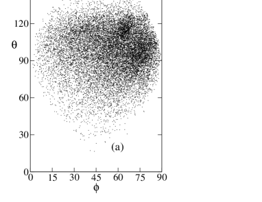
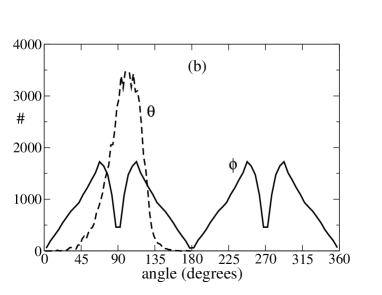
Figure 1: A scatter plot of $\theta$ vs. $\phi$ for the source population used in our simulations (a) as well as a distribution of those angles (b). $\theta$ is the polar angle between the relative velocity vector of the potential impactor and the Earth’s direction of motion and $\phi$ is an azimuthal location of the relative velocity (Valsecchi et al., 1999). These figures show that our distribution of possible impactors is not isotropic, a key assumption in many cratering theories. Only $\phi$ values from $0-90$${}^{\circ}\$are shown in (a) corresponding to post-pericenter encounters at ascending node; higher values of $\phi$ are simply mirror images of the scatter plot shown as all encounters have the same value of $\theta$ for a given object.

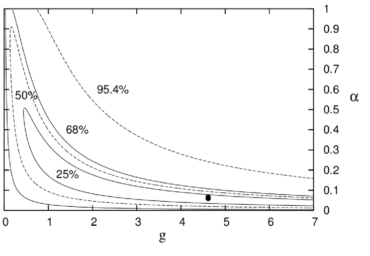
Figure 2: A contour plot of log(likelihood) values showing the degeneracy present in the parameters $\alpha$ and $g$ from Eq. 1 using the rayed crater data from Morota and Furumoto (2003). Best fit values for the rayed crater data are shown as the dot at $\alpha=0.063$ and $g=4.62$. This value for g gives the slope of the impactor mass distribution as $b=1.87$, over 3 times the observationally determined value of 0.58. However, a large range of $\alpha$ and $g$ values give acceptable fits to the data, making it impossible to measure the parameters of the projectile population from the crater distribution alone.

Because of the Moon’s small 1.0 km/s orbital velocity and standard literature values of $\bar{v}_{\infty}\sim 10-16$ km/s (Shoemaker, 1983; Chyba et al., 1994), one expects $\alpha\approx 1/16-1/10$ and thus a crater enhancement on the leading hemisphere in the range $\sim 1.4-1.7$, in terms of the GMAACA. Recent studies of young rayed craters (Morota and Furumoto, 2003; Morota et al., 2005) are found to be consistent with these estimates. We will calculate the GMAACA that current NEO impactors produce and compare with these values.

2.3 Lunar nearside/farside debate

The concept of a nearside/farside asymmetry has garnered less attention in the lunar cratering literature. Wiesel (1971) discussed the idea that the Earth would act as a gravitational lens, focusing incoming objects onto the nearside of the Moon. However, the degree to which this lensing effect occurs is unclear. The amplitude of nearside enhancement has been reported as insignificant (Wiesel, 1971), a factor of two (Turski, 1962; Wood, 1973), and most recently, a factor of four compared with the farside in a preliminary analysis by Le Feuvre and Wieczorek (2005). In contrast, Bandermann and Singer (1973) used analytic arguments to claim no a priori reason to expect such an asymmetry; the Moon may be in a region of convergent or divergent flux because the focal point of the lensed projectiles depends on the encounter velocity of the objects and the Earth-Moon distance. These latter authors estimated that there should currently be a negligible difference in the nearside/farside crater production rate. We will also investigate this issue as the initial conditions used in the previous dynamical studies were somewhat artificial.

3 Model and numerical methods

3.1 The source population

The cratering asymmetry expected on the synchronously-rotating Moon depends on the impactor speed distribution that is bombarding the satellite (the scalar $v_{\infty}\$distribution and its directional dependence). Therefore, we must have a model of the small-body population crossing Earth’s orbit. The potential impactors come from the asteroid-dominated (e.g., Gladman et al. (2000)) near-Earth object (NEO) population. The orbital distribution of these objects is best modeled by Bottke et al. (2002) who fit a linear combination of several main-belt asteroid source regions and a Jupiter-family comet source region to the Spacewatch telescope’s NEO search results. Since the detection bias of the telescopic system was included, this yields a model of the true NEO orbital-element distribution. W. Bottke (private communication, 2005) has provided us with an orbital-element sampling of their best fit distribution, which we have then restricted to 16307 orbits in the Earth-crossing region (Fig. 3). This will be our source population for the impactors which transit through the Earth-Moon system. We note the common occurrence of high eccentricity $e$ and inclination $i$ orbits in the NEO sample, which result in high values of $v_{\infty}\$for the bombarding population. Although semimajor axes $a$ in the $a$=2.0–2.5 AU region are densely populated (since this is the semimajor axis range of the dominant main-belt sources), impact probability is largest for orbits with perihelia $q=a(1-e)$ just below 1 AU or for aphelia $Q=a(1+e)$ just above 1 AU (Morbidelli and Gladman, 1998). Since the $q\sim 1$ population is much larger than the $Q\sim 1$ population, one might expect the former to dominate the impactors (but see Sec. 4.2).

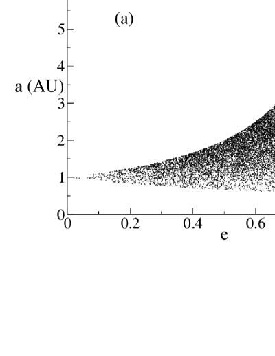
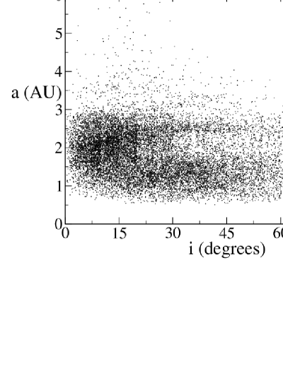
Figure 3: The orbital distribution of candidate impactors used in our simulations, based on the debiased near-Earth object (NEO) model of Bottke et al. (2002). We have used only objects whose perihelion $q$ and aphelion $Q$ satisfy $q\leq 1$ AU and $Q\geq 1$ AU. (a) Semi-major axis $a$ versus eccentricity, $e$. Note the increase in density near $a\sim 2.5$ AU due to the 3:1 orbital resonance with Jupiter. (b) Semi-major axis versus inclination $i$ with respect to the ecliptic.

3.2 Setup of the flyby geometries

The orbital model provides only the $(a,e,i)$ distribution of the NEO population and we expect that the 1.7% eccentricity of the Earth’s orbit is a small correction to the impactor distribution, so for what follows we have modeled the Earth’s heliocentric orbit as perfectly circular. As a result we can, without loss of generality, take all encounters to occur at (1 AU,0,0) in heliocentric coordinates, where we have lost knowledge of the day of the year of the encounters (although we can easily average over the year by post-facto selecting a random azimuth for the Earth’s spin pole at the time of a projectile’s arrival at the top of the atmosphere). With this restriction, each Earth-crossing orbit can have an encounter in one of four geometries depending on the argument of pericenter $\omega$ and the true anomaly $f$, which must satisfy:

$$r=1~{}\mathrm{AU}=\frac{a(1-e^{2})}{1+e\cos f}\;\;\;.$$ (5)

By construction, the encounter must occur at either the ascending or descending node along the $x$-axis, and so the longitude of ascending node is $\Omega$=0 or $\pi$. Taking $f$ and $\omega$ in $[0,2\pi)$, for ascending encounters, $f=2\pi-\omega$ for either encounters with pericenters above ($\omega=[0,\pi)$) or below ($\omega=[\pi,2\pi)$) the ecliptic. If the encounter occurs at the descending node, $f=\pi-\omega$ for post-pericenter encounters and $f=3\pi-\omega$ for pre-pericenter encounters. With this in mind, we effectively quadruple the number of initial conditions to 65228.

With the longitude of ascending node fixed (ie. $\Omega=0\mathrm{\ or\ }\pi$), we then construct a plethora of incoming initial conditions based on the orbital elements from the debiased NEO model converted to Cartesian coordinates. For each initial orbit, all four of the encounter geometries are equally likely. We randomly choose a particle for a flyby based on its encounter probability with the Earth as judged by an Öpik collision probability calculation (Dones et al., 1999). Gravitational focusing by the Earth was not included in the encounter probability estimate as an increased frequency of Earth deliveries will occur naturally during the flyby phase if the Earth’s gravity is important.

Both Earth and a test particle (TP) are then placed at the nodal intersection and moved backwards on their respective orbits until the separation between the NEO and the Earth is 0.02 AU. At this point, we create a disk of $10^{5}$ non-interacting test particles, meant to represent potentially-impacting asteroids or comets, centered on the chosen orbit. A short numerical integration is run for each of the 65228 initial conditions and one TP trajectory that results in an arrival at the Earth in each flyby is placed into a table of new initial conditions. This procedure is performed because during the “backup phase” to separate the Earth and TP by 0.02 AU, gravitational focusing was not accounted for. The omission could result in the particle missing the Earth in a forward integration, as the Earth’s gravity would be present, modifying the chosen trajectory. This gives us a final set of 65228 initial trajectories that strike the Earth when a forward integration is performed. For convenience we then convert from heliocentric coordinates to a geocentric frame of reference.

For our simulations, one of the new initial conditions is randomly chosen based on a newly calculated encounter probability with the Earth-Moon system. A new disk, centered on the chosen trajectory, is randomly populated with $10^{5}$ test particles, all given identical initial velocities. The radius of the disk is chosen to be 2.5 lunar orbital radii as testing showed that for all of our initial conditions, a disk of this size spans the entire lunar orbit as it passes the Earth’s position. This was done to ensure the crater distribution had no dependence on the lunar orbital phase. Figure 4 shows a schematic of the simulations.

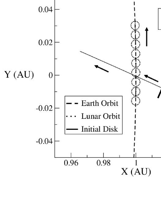
Figure 4: A schematic of one 3-dimensional flyby projected onto the ecliptic in a heliocentric coordinate frame. A disk (thick, solid line) of $10^{5}$ test particles, all with identical initial velocities, is created around a central trajectory based on the NEO source population of Bottke et al. (2002). The disk is 2.5 lunar orbital radii in radius and encompasses the entire lunar orbit for any of our possible initial conditions. These test particles are then integrated forward along with the Earth, Moon, and Sun and have an encounter with the Earth-Moon system near (1 AU,0,0). All particles are followed for three times the amount of time required for the farthest test particle to reach the Earth.

3.3 Integration method

The orbital trajectories of the massive bodies (Earth, Moon and Sun) and the TPs are integrated using a modified version of swift-rmvs3 (Levison and Duncan, 1994). The length units are in AU and time units are in years. The initial eccentricity and inclination for both the Earth and Moon are set to zero for the majority of our simulations. In one run we introduce the current 5.15${}^{\circ}\$inclination of the Moon, keeping Earth’s $e$ and $i$ as before.

Both Earth and Moon are assumed to be perfect spheres. Factors that vary in the simulations include the number of flybys, where a flyby is defined as a disk of $10^{5}$ test particles passing through the Earth-Moon system, and the Earth-Moon distance, $R_{EM}$.

We have the Earth as the central body with the Moon acting as an orbiting planet and the Sun as an external perturber. The base time step in the simulations is four hours. This is large enough to not be time prohibitive, but small enough such that the integrator can follow the lunar encounters precisely. During the course of the integration, the integrator logs the positions and velocities of all bodies of interest if there is a pericenter passage within the radius of the Moon or Earth.

We then use this log as input for a backwards integration using a $6^{th}$-order explicit symplectic algorithm (Gladman and Duncan, 1991) to precisely determine the latitude and longitude of the particle’s impact location. This method, along with iterative time steps, enables us to find impact locations to within 5 km of the surface of the Moon and within $<500$ m of the top of Earth’s atmosphere.

This project is computationally intensive. For each simulation, the Earth, Moon and Sun are included as well as $10^{5}$ test particles. Each of the 65228 initial conditions are used multiple times to improve statistics and in each case the TP locations in the disk are randomly distributed. Thus more than $2\times 10^{12}$ test particles are integrated which results in tens of millions of terrestrial deliveries and hundreds of thousands of lunar ones.

4 Delivery to Earth

Before turning to the Moon, we examine our numerical results to determine the spatial distribution of Earth arrivals. Our simulations with the Moon at the current orbital distance of $60R_{\oplus}$ yielded 21,998,427 terrestrial impacts. Since the crater record on the Earth is difficult to interpret due to geological processes, we choose to examine our results in terms of fireball and meteorite records as the impactors strike the top of the atmosphere. We are thus assuming that the meteorite dropping bodies have a pre-atmospheric orbital distribution similar to the NEOs (but see Sec. 4.2).

Figure 5 shows velocity distributions for the Earth arrivals from our simulations. The delivery speeds should be interpreted as “top of the atmosphere” velocities, $v_{imp}$. The deliveries are dominated by low $v_{\infty}\$objects which the Earth’s gravitational well has focused and sped up, creating a peak in the distribution at a speed of $\sim 15$ km/s. The average speed an impactor has at the top of the atmosphere is $\sim 20$ km/s, slightly higher than the often quoted value of 17 km/s (Chyba et al., 1994). As well, if we compare our Fig. 5 to the fireball data in Morbidelli and Gladman (1998, Fig. 8a), we see a general similarity in the shapes of the $v_{imp}$ histograms.

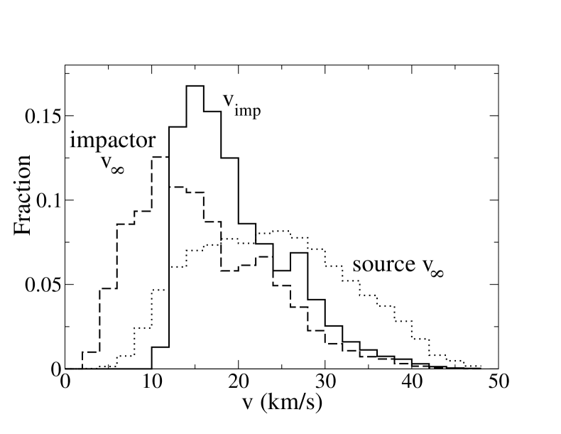
Figure 5: Velocity distributions for the Earth deliveries from our simulations (impactor $v_{\infty}\$and $v_{imp}$) as well as the sampled NEO population (source $v_{\infty}\$). Note that the average impact velocity is $\sim$ 20 km/s, higher than the often-quoted value of $17$ km/s. One can observe the large effect of the Earth’s gravitational well for $v_{\infty}\$values $\lesssim 10$ km/s. Here the encounter speeds are “pumped up” to values slightly higher than the Earth’s escape velocity of 11.2 km/s. From the $v_{\infty}\$distribution of $all$ possible impactors it is clear that the impacts are dominated by low ($v_{\infty}\$$\lesssim 20$ km/s) objects.

4.1 Latitude distribution of delivered objects

For a uniform spatial distribution of deliveries, one expects the number of arrivals to vary as the cosine of the latitude due to the smaller surface area at higher latitudes. Figure 6 shows that to an excellent approximation, the Earth is uniformly struck by impactors (in latitude). To account for the area in each latitude bin, divide by:

$$A_{bin}=2\pi R_{\oplus}^{2}(\cos\theta_{1}-\cos\theta_{2}),$$ (6)

where the co-latitudes $\theta_{1}>\theta_{2}$ are measured north from the south pole.

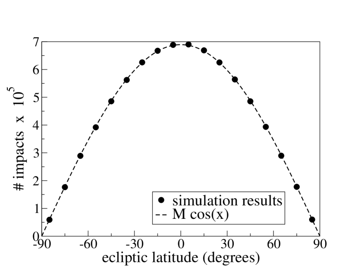
Figure 6: A latitude distribution of projectile deliveries to the Earth from one set of simulations. This figure has not accounted for the spin obliquity of the planet (hence “ecliptic latitude”). The points represent the total number of impacts in $10^{\circ}$ ecliptic latitude bins and the dashed curve is a cosine multiplied by an arbitrary constant, $M$. The error bars for the simulation results are smaller than the points.

To correct for the spin obliquity of the Earth, we then choose a random day of fall, and thus a random azimuth for the Earth’s spin pole. This then gives us a geocentric latitude and longitude for each simulated delivery. Figure 7 shows the spatial density versus geocentric latitude. For the long-term average, we see a nearly uniform distribution of arrivals. If we restrict to azimuths corresponding to northern hemisphere spring or northern hemisphere autumn, we see the well-known seasonal variation (Halliday and Griffin, 1982; Rendel and Kn$\ddot{\mbox{o}}$fel, 1989) in the fireball flux of roughly 15% amplitude (Fig. 7). As a measure of the asymmetry between the poles and equator, we take the ratio between polar (within 30${}^{\circ}\$of the poles) and equitorial (a 30${}^{\circ}\$band centered on the equator) arrival densities. We find that when all terrestrial arrivals are considered, the poles receive the same flux of impactors as the equator to $<1$% ($0.992\pm 0.001)$. We believe the uncertainty caused by our finite sampling of the orbital distribution is on this level and thus our results are consistent with uniform coverage.

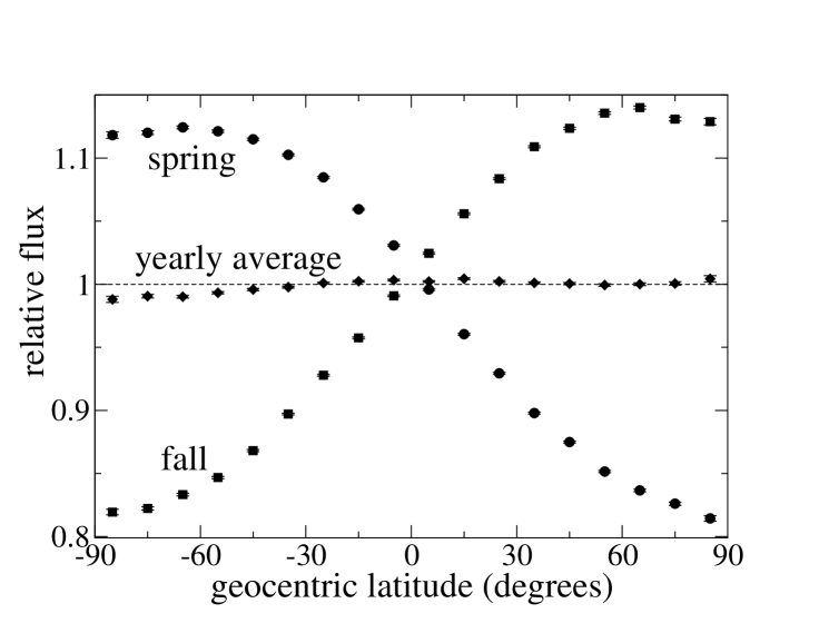
Figure 7: The geocentric latitude distribution, relative to the average spatial density of impacts, at different times of the year. The circles represent northern hemisphere spring, when the Earth’s spin axis (as viewed from above) is tilted away from the planet’s direction of motion. The near mirror-image can be seen in northern hemisphere fall (squares) when the spin axis is tilted towards the Earth’s direction of motion. Averaged over a full year (diamonds), the deviation from the expected flat distribution is minimal.

To better understand the details of latitudinal asymmetries, we consider the effect of approach velocity, $v_{\infty}\$. When our projectile deliveries are filtered such that $v_{cut1}\leq v_{\infty}\leq v_{cut2}$, and restricted to impactors with $i\leq 10$${}^{\circ}\$we find results similar to Le Veuvre and Wieczorek (2006, our Fig. 8a can be compared to their Fig. 2). Their $N_{g}$ parameter is analogous to our $v_{\infty}\$cuts. Small encounter velocities produce more uniform coverage because the trajectories are bent towards the poles. Higher encounter velocity trajectories are not effected to as great a degree and tend to move in nearly straight lines, leading to a distribution which tends to a cosine-like curve. Obviously when the $i$ restriction is lifted, the poles receive a higher flux which mutes the amplitude of the variation (Fig 8b).

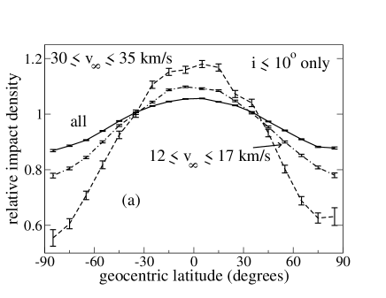
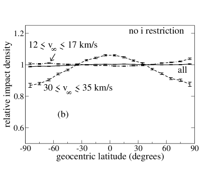
Figure 8: The terrestrial impact density versus geocentric latitude (a) for different ranges of encounter velocity $v_{\infty}\$and restricted to objects with inclination $\leq 10$${}^{\circ}\$and (b) the same with no inclination restriction. For lower $v_{\infty}\$objects, there is less latitudinal variation because the Earth’s gravitational field bends incoming trajectories towards higher latitudes. This effect is muted as the velocities become larger - the trajectories move in straighter lines. For these faster objects, the available impact area varies as a cosine so the shape of the distribution for high $v_{\infty}\$impactors is expected to do the same. The deviations from a cosine are due to the fact the objects have moderate inclinations and non-infinite velocities. Note that (b) shows the realistic case of all encounter speeds and inclinations; there is very little latitudinal variation.

The preliminary results of Le Feuvre and Wieczorek (2006) show a 30% ecliptic latitudinal variation in terrestrial projectile deliveries. Though we are able to produce results similar to theirs under various restrictions (Fig. 8a), the inclusion of the Earth’s spin obliquity is necessary to accurately reflect reality. With this inclusion, we find a latitude distribution which is very nearly uniform (Fig. 8b).

4.2 AM/PM asymmetry

The ecliptic latitudes and longitudes for the terrestrial arrivals were converted into local times via a straightforward method. As stated in the previous section, the Earth’s spin-pole azimuth is chosen at random to represent any day of the year and then the arrival location is transformed to these geocentric coordinates. The location relative to the sub-solar direction gives the local time.

We looked for a PM excess in our simulation results. However, as evident in Fig. 9a we see the opposite effect. Previous modeling work produced a near mirror image (reflected through noon) of our result (see our Fig. 9b and Fig. 3 of Halliday and Griffin (1982)), but their impactor orbital distribution was very different from the debiased NEO model; they chose a small set of orbits with perihelion $q$ in the range $0.62\leq q\leq 0.99$ AU with semimajor axis $a$ obeying $1.3\leq a\leq 3.2$ AU. If we restrict our simulation results to approximately the same impactor distribution (by taking only those objects having $a$ and $q$ within $\pm\ 0.01$ AU of the entries in Table 1 of Halliday and Griffin (1982)), we obtain Fig. 9b which is very similar to their result.

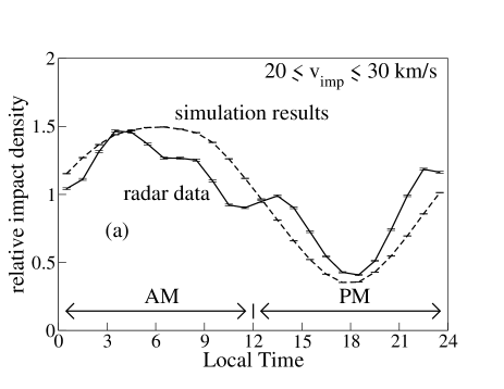
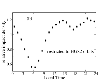
Figure 9: The local time distribution of arrivals at the top of Earth’s atmosphere for both our simulations and radar data (a). The simulation deliveries have been corrected for the Earth’s spin obliquity. Clearly there is a large AM excess in the arrivals which is counter to the meteorite fall data which show a PM enhancement. Though a velocity restriction is used (see text), other cuts yield the same general shape for both radar data and simulation results. (b) The local time distribution of Earth deliveries when restricted to orbits similar to the ones used in Halliday and Griffin (1982). This distribution matches well with the time of falls for chondrites.

Why is there this discrepancy with our unrestricted case? The origin is not one of method but rather of starting conditions. The debiased NEO model we use is much more comprehensive than the orbits used by Halliday and Griffin (1982), where only orbits assumed to represent then-current fireballs were included. The real Earth-crossing population contains a larger fraction of high-speed orbits, which produce a smaller fraction of PM falls than the shallow Earth-crossers. In fact, our simulated arrivals always show an AM excess (Fig. 10), even if we apply an upper speed bound (in an attempt to mimic a condition for meteoroid survivability, requiring speeds of less than 20–30 km/s at the top of the atmosphere).

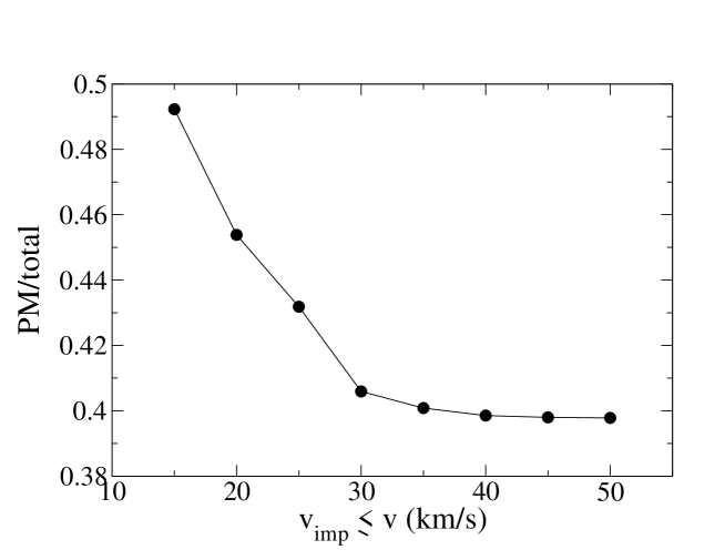
Figure 10: The fraction of Earth arrivals on the PM hemisphere, as a function of various cutoff speeds in the incoming flux. For the entire population, the PM ratio is 40%. Applying more and more stringent upper bounds pushes the PM ratio towards 50%, but for reasons discussed in the text we do not believe that the NEO orbital distribution is the same as that of meteorite-dropping fireballs, and thus the AM excess we find (which is not exhibited by the fireball data as a whole) does not create a contradiction with the available data.

The apparent conflict with the meteorite data should not be too surprising, as Morbidelli and Gladman (1998) argued that that orbital distribution of the 0.1–1 m-scale meteoroids that drop chondritic fireballs must be different than that of the Near-Earth Objects. They showed that to match the radiant and orbital distributions determined by the fireball camera networks and to also match a PM excess, these sub-meter sized bodies must suffer strong collisional degradation as they journey from the asteroid belt, with a collisional half life consistent with what one would expect for decimeter-scale objects; this produces a match with the fireball semimajor axis distribution, which is dominated by the $a>1.5$ AU orbits. In contrast, our simulations show NEO arrivals are much more dominated by $a\sim 1$ AU objects. We posit this is further evidence that the source region for the majority of the meteorites (the chondrites) is the main belt and not near-Earth space; to use the terminology of Morbidelli and Gladman (1998), the ‘immediate precursor bodies’, in which the meteoroids were located just before being liberated and starting to accumulate cosmic-ray exposure, are not near-Earth objects but must be in the main belt.

As a consistency check, we compare our fall time distribution to radar observations (Jones et al., 2005) of meteoroids arriving at the top of Earth’s atmosphere. Figure 9a shows that the fall time distribution obtained with our simulations is similar to the flux of radar-observed meteors when restricted to the same top-of-the-atmosphere speed range of $20\leq v_{imp}\leq 30$ km/s (though other cuts yield similar results). The typical pre-atmospheric masses of the particles producing the radar meteors is in the micro- to milli-gram range (P. Brown, private communication 2006). The velocity range chosen for Fig. 9a removes the low-speed fragments which have reached Earth-crossing by radiation forces (unlike the NEOs of the Bottke model, whose orbital distribution is set by gravitational scatterings with the terrestrial planets) and also removes the high-speed cometary component.

The match we find permits the hypothesis that the majority of the milligram-particle flux on orbits with these encounter speeds is actually dust that is liberated continuously from NEOs, in stark contrast with the decimeter-scale meteoroids, who must be recently derived from a main-belt source.

5 Lunar bombardment

Figure 11 shows the lunar impact speed distribution from our simulations. Because the Moon’s orbital and escape speeds (1.02 and 2.38 km/s respectively) are both small compared to typical $v_{\infty}\$encounter speeds, the impacts are not as biased towards smaller speeds as for the Earth. As one would expect, since $v_{imp}^{2}=v_{\infty}^{2}+v_{esc}^{2}$, the $v_{imp}$ and source $v_{\infty}\$distributions are quite similar. The small difference arises from gravitational focusing by the Moon, which increases the speeds of the low $v_{\infty}\$population. We compute the average impact speed for NEOs striking the moon to be 20 km/s. This is higher than the often quoted lunar impact velocity of 12-17 km/s (Chyba et al., 1994; Strom et al., 2005). These lower velocities have been derived using only the known NEOs and are therefore biased towards objects whose encounter speeds are lower (which are more often observed in telescopic surveys).

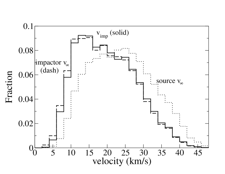
Figure 11: Velocity distributions for the lunar impacts from our simulations (impactor $v_{\infty}\$and $v_{imp}$) and the sampled NEO source population (source $v_{\infty}\$). The average impact velocity, is $\sim$ 20 km/s. The curve showing the $v_{\infty}\$of objects striking the Moon closely matches the $v_{imp}\$distribution as one expects due to the small degree at which the moon’s gravity well “speeds up” low $v_{\infty}\$objects. The difference between the $v_{imp}$ and source $v_{\infty}\$distributions shows that gravitational focusing favours low speed ($v_{\infty}\$$\lesssim 20$ km/s) objects. These simulation results were for the current Earth-Moon distance with the Moon orbiting in the plane of the ecliptic.

The debiased NEO distribution we use has a full suite of high-speed impactors; more than half the impactors are moving faster than $v_{med}$ = 19.3 km/s when they hit the Moon. This has serious implications for the calculated projectile diameters that created lunar craters since the higher speeds we calculate mean that typical impactor diameters are smaller than previously derived. Strictly speaking, our results apply only when the current NEO orbital distribution is valid, which has likely been true since the post-mare era. However, the generically-higher lunar impact speeds we find are likely true in most cases for realistic orbital distributions, and thus the size-frequency distribution of the impactors must be shifted to somewhat smaller sizes in trying to find matches between the lunar crater distribution and the NEA size distribution (see Strom et al 2005 for a recent example).

The reader may be surprised to see that the average lunar impact speed is essentially the same as the average arrival speed at Earth despite the acceleration impactors receive as they fall into the deep gravity well of our planet. This (potentially counter-intuitive) result can be understood once one realizes that Earth’s impact speed distribution is heavily weighted towards low $v_{\infty}\$values by the Safronov factor $(1+v_{esc}^{2}/v_{\infty}^{2})$. For Earth this so heavily enhances the low encounter speed impactors that the average impact speed actually drops to essentially the same as that of the Moon (which does not gravitationally focus the low $v_{\infty}$ nearly as well). While the Earth’s greater capture cross-section ensures a much larger total flux, the average energy delivered per impact will be similar for both the Moon and Earth.

5.1 From impacts to craters

To examine crater asymmetries on the Moon, we need to convert our simulated impacts (a sample of which are shown in Fig. 12) into craters which will account for the added asymmetry resulting from the impact velocity $v_{imp}$ of the impactors. In typical crater counting studies, there is some minimum diameter $T$ which observers are able to count down to due to image resolution limitations. There will be more craters larger than $T$ on the leading hemisphere than on the trailing because leading-side impactors have higher impact speeds on average and the commonly-accepted scaling relation for crater size $D_{c}$ depends on the velocity.

$$D_{c}\propto v_{imp}^{2q}\;D_{i}^{3q}\;,$$ (7)

where $q\approx 0.28-0.33$ (Melosh, 1989) and $D_{i}$ is the diameter of the impactor. Since both hemispheres receive flux from the same differential impactor size distribution obeying

$$\frac{dN}{dD_{i}}\propto D_{i}^{-p}\;,$$ (8)

we can integrate “down the size distribution” to determine a weighting factor which transforms our impacts into crater counts. The number of craters $N$ with $D_{c}>T$ produced by the impacting size distribution is

$$N(D_{c}>T)\>=\>\int_{D_{imin}}^{\infty}\frac{dN}{dD_{i}}\>dD_{i}\>=\>\frac{1}{p-1}\;D_{imin}^{1-p}\>\propto\>v_{imp}^{2(p-1)/3}\;,$$ (9)

where $D_{imin}$ is some minimum impactor diameter and we have substituted $D_{imin}\propto(T\;v_{i}^{-2q})^{1/3q}$. Since the differential size index $p\sim 2.8$ (Stuart, 2001; Bottke et al., 2002), $N\propto v_{imp}^{1.2}$.

For each simulated impact at a specific latitude and longitude, we assign that impact $N=C\;v_{imp}^{1.2}$ craters, where $C$ is an arbitrary proportionality constant. The dependance on $p$ is small as our results are essentially the same when using an older determined value of $p=2$. The weak dependance arises from the low orbital speed of the Moon relative to the encounter speeds of the incoming projectiles. Thus for moons such as the Galilean satellites, whose orbital speeds are much higher compared to that of the incoming flux, the value for $p$ becomes more important. Note that $D_{min}$ and $q$ are actually irrelevant to our analysis since we are interested in only the crater numbers relative to an average rather than the crater sizes.

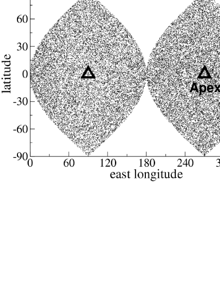
Figure 12: An equal-area projection of the lunar impacts from our simulations. The Moon was at its current orbital distance of $60R_{\oplus}$ with 0${}^{\circ}\$inclination. At the apex, one can see the slight enhancement in the impact density. For clarity, only 7% of the total number of impacts are shown.

5.2 Latitude distribution of impacts

One expects the departure from uniform density in the lunar latitude distribution to be more severe than that of the Earth due to the Moon’s smaller mass. Comparing Fig. 13 to Fig. 8b shows this is indeed the case. At high $v_{\infty}\$cuts, the variation in the latitude distribution tends to the predicted cosine (see Fig. 2 in Le Feuvre and Wieczorek, 2006). However, when examining the real case of all lunar impacts we see only a $\sim 10$% ($0.912\pm 0.004$) depression at the poles when taking the ratio of the derived crater density within 30${}^{\circ}\$of the poles to the crater density in a 30${}^{\circ}\$band centered on the equator. In contrast, Le Feuvre and Wieczorek (2006) (their Fig.3) find a polar/equatorial ratio of roughly 60%. The source of this large discrepancy is unclear since the Moon in our simulations had zero orbital inclination and spin obliquity, the same conditions used by Le Feuvre and Wieczorek (2006), and the latter also used the Bottke et al. (2002) model as an impactor source. Despite the variation we observe being small, researchers should be aware of this spatial variation in the crater distribution when determining ages of surfaces (see Sec. 6).

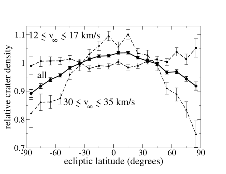
Figure 13: The latitude distribution of craters on the Moon from our simulations. Note the scale is different here than in Fig. 8(b) and that the latitudinal variation is larger for the Moon than the Earth. This is because the Moon’s gravity well is not deep enough to significantly modify incoming trajectories to higher latitudes. If the impacts were restricted to impactors which had $i\leq 10$${}^{\circ}\$, the variation would be larger as is the case with the terrestrial deliveries in Fig. 8. Here the Moon’s inclination and spin obliquity are not accounted for.

5.3 Longitudinal effects

We wish to compare the results of our numerical simulations with observational data to create a consistent picture of the current level of cratering asymmetry between the Moon’s leading and trailing hemispheres. As a measure of this asymmetry, we look at the crater density as a function of the angle away from the apex, $\beta$, which should roughly follow the functional form of Eq. 1. In Fig. 14 we show the results from our simulations as well as a fit to Eq. 1 using a maximum likelihood technique assuming a Poisson probability distribution. The best fit parameters resulting from an unrestricted analysis are $\bar{\Gamma}=1.02$, $\alpha=0.564$, and $g=0.225$; this would require $b=-1.268$. For an impactor diameter distribution following $\frac{dN}{dD}\propto D^{-b}$, this value for the slope yields the unphysical situation of having more large impactors than small ones. Obviously this cannot be correct and is a consequence of the degeneracy present in Eq. 1. We once again conclude that by fitting Eq. 1 to an observed surface distribution, it is virtually impossible to decouple $\alpha$ and $g$ to obtain information about the impactor size distribution and the average encounter velocity of the impactors.

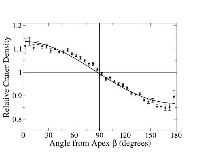
Figure 14: The spatial density of simulated craters as a function of angle from the apex of motion, $\beta$. The vertical axis is craters/$\mathrm{km}^{2}$ relative to the mean density over the entire lunar surface. Points represent simulation results while the curve gives a fit using a maximum likelihood technique to the equation $\Gamma(\beta)=\bar{\Gamma}(1+\alpha\cos\beta)^{g}$, where $g=2+1.4\;b$ and $b=0.58$ as determined from observations. With this restriction, the best fit values are $\bar{\Gamma}=0.994$ and $\alpha=0.0472$ with a reduced chi-square of $\bar{\chi}_{r}^{2}=2.4$.

By counting our simulated craters, we find a value for the GMAACA of $1.29\pm 0.01$, significantly lower than the values of 1.4–1.7 estimated in Sec. 2.2. This discrepancy can be reconciled by recalling that we find the average impactor $v_{\infty}\$to be $\sim$ 20 km/s. Using this value in Eq. 2 and the observationally-determined value of $b=0.58$, gives a GMAACA value of 1.32, close to the value we obtain. In Fig. 14 we notice that the distribution is rather flat for $0^{\circ}\leq\beta\leq 45^{\circ}$ and has higher density than the predicted curve (using $b=0.58$) for $60^{\circ}\leq\beta\leq 120^{\circ}$. A $\bar{\chi}_{r}^{2}$ value of 2.4 results when the quality of fit is assessed. We believe the origin of this highly-significant departure from the theoretically predicted form lies simply in the fact that both assumptions of an (1) isotropic orbital distribution of impactors with (2) a single $v_{\infty}\$value, are violated (see Fig. 1). Thus, an observed crater field will not follow the form of Eq. 1 in detail.

Since these assumptions break down for the real impactor population, we will instead directly compare with the rayed crater observations to determine if the available data rule out our model. To do this, we scaled our craters down to 222, the same number as in the rayed crater sample used in Morota and Furumoto (2003). We restricted our simulated craters to the same lunar area examined in that study. Mare regions were ignored as it introduces bias in rayed crater observations because they are easier to identify against a darker background surface. In addition, rayed craters on mare surfaces are likely older than their highland counterparts because it takes longer for micrometeorite bombardment to eliminate the contrast. Since we are interested in the current lunar bombardment, it is necessary to eliminate this older population. The area sampled includes latitudes $\pm 41.5$${}^{\circ}\$and longitudes $70.5$${}^{\circ}\$$-\>289.5$${}^{\circ}\$(see Fig. 1 of Morota and Furumoto, 2003). Using a modified chi-square test with the rayed crater observational counts $O_{i}$ and the expected counts $E_{i}$ from our simulations,

$$\chi^{2}=\sum_{i}^{n}\frac{(O_{i}-E_{i})^{2}}{\sigma_{obs}^{2}},\mathrm{\;\;with\;\;}\sigma_{obs}=\sqrt{O_{i}}$$

since we are dealing with Poisson statistics. This procedure results in a reduced chi-square value of $\bar{\chi}_{r}^{2}=0.67$. Thus our model is in excellent agreement with the observational data (Fig. 15).

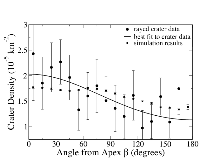
Figure 15: Density of rayed craters used in Morota and Furumoto (2003) compared with our simulation results for the same lunar area and scaled to the same count (222). The curve is the best fit to the rayed crater data using Eq. 1 as a model despite our knowledge that it is based on violated assumptions. Best fit parameters are $\bar{\Gamma}=1.53\times 10^{-}5\;\mathrm{km}^{-2},\;\alpha=0.063,\;\mathrm{and}\;g=4.62$. With respect to the observations, the prediction from our numerical calculations has $\bar{\chi}_{r}^{2}=0.67$.

Ideally, we would like to obtain a GMAACA value for the rayed crater data. However, due to small number statistics and the restricted area (because of Mare Marginis and Mare Smythii, much of the area near the the antapex is excluded), the GMAACA value is poorly measured by the available data. Regardless, integrating the best fit of the rayed crater data (best fit values: $\bar{\Gamma}=1.53\times 10^{-5}\;\mathrm{km}^{-2},\;\alpha=0.063,\;g=4.62,\;\mathrm{with}\;\bar{\chi}_{r}^{2}=0.49$) from 0-30${}^{\circ}\$and 150-180${}^{\circ}\$to form the GMAACA ratio gives $1.7_{-0.6}^{+0.9}$, consistent with our result.

5.4 Varying the Earth-Moon distance and the effect of inclination

Due to tidal evolution, in the distant past the Moon’s orbit was smaller. As the orbital distance is decreased, the Moon’s orbital speed rises. This increases the impact speeds on the leading hemisphere and makes “catching up” to the Moon from behind more difficult. As Eq. 2 suggests, the degree of apex/antapex asymmetry on the Moon is expected to increase as the orbital speed of the satellite does. We examined this by running other simulations with an Earth-Moon separation of $a=$50, 38, 30, 20, and 10 $R_{\oplus}$. Figure 16 shows our results. Assuming the same impactor orbital distribution in the past, only a mild increase in the apex enhancement is seen (since the orbital speed only increases as $1/\sqrt{(}a)$). The increase is that expected based on the resulting change in $\alpha$ caused by the larger $v_{orb}$ (see Eq. 2).

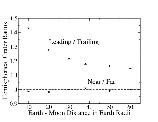
Figure 16: The ratio between number of craters on the leading versus trailing hemispheres and the same ratio between the nearside and farside hemispheres as a function of lunar orbital distance. As expected, smaller orbital distances increase the asymmetry between leading and trailing hemispheres. This is a result of the increased orbital speed as the Moon is brought closer to the Earth. For all lunar distances there is minimal nearside/farside asymmetry, with some evidence the Earth shielded the lunar nearside in the very distant past when the lunar semimajor axis was $<\;25\;R_{\oplus}$.

As discussed in Sec. 2.3, the asymmetry between the near and far hemispheres should depend on the lunar distance. Figure 16 shows the ratio between nearside and farside craters from our simulations. For all lunar distances we find very little asymmetry. Thus, our results do not support the most recent study which claims a factor of four enhancement on the nearside when compared to the far (Le Feuvre and Wieczorek, 2005), but are in good agreement with the work done by Wiesel (1971) and Bandermann and Singer (1973). We see mild evidence for Bandermann and Singer’s (1973) assertion of the Earth acting as a shield for $a<25R_{\oplus}$ and little effect outside this distance. Thus, Bandermann and Singer’s estimate of no measurable nearside/farside asymmetry in the current cratering rate is correct.

In the bulk of our simulations we have used the approximation that the Moon’s orbit is in the ecliptic plane. Since we show that the latitudinal dependence of lunar cratering is weak ($\sim$ 10% reduction within 30^∘ of the poles relative to a 30${}^{\circ}\$band centered on the Moon’s equator), we do not expect the inclusion of the moon’s orbital inclination to alter our results significantly, although we expect the polar asymmetry to monotonically decrease with increasing orbital inclination. We have confirmed this by computing the GMAACA and polar asymmetry ratios for a less-extensive set of simulations in which the lunar orbital inclination is initially set to its current value of 5.15^∘ and we use the sub-Earth point at the time of impact to compute lunocentric latitudes and longitudes. We find a slight reduction of GMAACA to $1.24\pm 0.02$ from ($1.29\pm 0.01$) and a crater density within 30^∘ of the pole that is statistically the same as the 0${}^{\circ}\$inclination case ($0.914\pm 0.009$ instead of $0.912\pm 0.004$).

6 Summary and conclusions

We have used the debiased NEO model of Bottke et al. (2002) to examine the bombardment of the Earth-Moon system in terms of various impact and crater asymmetries. For Earth arrivals we find a $<1$% variation in the ratio between the areal densities within 30${}^{\circ}\$of the poles and within a 30${}^{\circ}\$band centered on the equator. The local time distribution of terrestrial impacts from NEOs is enhanced during the AM hours. While this fall-time distribution corresponds well to recent radar data, it is in disagreement with the chondritic meteorite data and their derived pre-atmospheric orbital distributions. This discrepancy thus reinforces the conclusion of Morbidelli and Gladman (1998) that the large amount of decimeter-scale material being ejected from the main asteroid belt onto Earth-crossing orbits must be collisionally depleted before much of it can evolve to orbits with $a<1.5$ AU.

A significant result is that we find the average impact speed onto the Moon to be $\bar{v}_{imp}=20$ km/s, with a non-negligible higher-speed tail (Fig. 11). This combined with quantification of the non-uniform surface cratering has implications for both tracing crater fields back to the size distribution of the impactors and the absolute (or relative) dating of cratered surfaces. First, the higher impact speeds we find mean that lunar impact craters (at least in the post-mare era when we believe the NEO orbital distribution we are using is valid) have been produced by smaller impactors than previously calculated. This roughly 10% higher average impact speed corresponds to lunar impactors which are 10% smaller on average than previously estimated; this small correction has ramifications for proposed matches between lunar crater size distributions and impactor populations (e.g., Strom et al.2005).

We find two different spatial asymmetries in current crater production due to NEOs. As expected, due to its smaller mass, the Moon exhibits more latitudinal variation ($\sim 10$%) in our simulations than the Earth. When comparing our simulation results to young rayed craters on the Moon, the surface density variation we predict is completely consistent with available data; we obtain a leading versus trailing asymmetry of $1.29\pm 0.01$ (GMAACA value), which corresponds to a 13% increase (decrease) in crater density at the apex (antapex) relative to the average. These results indicate that using a single globally-averaged lunar crater production could give ages in error by up to 10% depending on the location of the studied region. For example, post-mare studies of the Mare Orientale region would overestimate its age by $\sim 10$% due to its proximity to the apex, assuming that leading point and poles of the Moon have not changed over the last $\sim$4 Gyr. Similarly, the degree of bombardment on Mare Crisium (not far from the antapex) would be lower than the global average. These effects will only be testable for crater fields with hundreds of counted craters so that the Poisson errors are small compared to the 10% variations we find; in most studies of “young” ($<4$ Gyr) lunar surfaces the crater statistics are poorer than this (e.g., Stöffler and Ryder 2001).

When the orbital distance of the Moon was decreased (as it was in the past because of its tidal evolution), the ratio between simulated craters on the leading hemisphere versus the trailing increased as expected due to the higher orbital speed of the satellite at lower semi-major axes. We find virtually no nearside/farside asymmetry until the Earth-Moon separation is less than 30 Earth-radii, which under currently-accepted lunar orbital evolution models dates to the time before 4 Gyr ago (at which point the current NEO orbital distribution may not be a good model for the impactors). Interior to 30 Earth-radii we find that the Earth serves as a mild shield, reducing nearside crater production by a few percent.

Acknowledgments

Computations were performed on the LeVerrier Beowulf cluster at UBC, funded by the Canadian Foundation for Innovation, The BC Knowledge Development fund, and the UBC Blusson fund. BG and JG thank NSERC for research support.

References

- Bandermann and Singer (1973) Bandermann, L. W., and Singer, S. F. 1973. Calculation of meteoroid impacts on Moon and Earth. Icarus 19, 108-113.
- Barricelli and Metcalfe (1975) Barricelli, N. A., and Metcalfe, R. 1975. A note on the asymmetric distribution of the impacts which created the lunar mare basins. The Moon 12, 193-199.
- Bottke et al. (2000) Bottke, W. F., Jedicke, R., Morbidelli, A., Petit, J.-M., and Gladman, B. 2000. Understanding the distribution of near-Earth asteroids. Science 288, 2190-2194.
- Bottke et al. (2002) Bottke, W. F., Morbidelli, A., Jedicke, R., Petit, J.-M., Levison, H. F., Michel, P., and Metcalfe, T. S. 2002. Debiased orbital and absolute magnitude distribution of the near-Earth objects. Icarus 156, 399-433.
- Chyba et al. (1994) Chyba, C. F., Owen, T. C., and Ip W. -H. 1994. Impact delivery of volatiles and organic molecules to Earth. Hazards Due to Comets Asteroids. Space Science Series, Tuscon, AZ: Edited by Tom Gehrels, M. S. Matthews. and A. Schumann. Published by University of Arizona Press, 1994., p.9.
- Dones et al. (1999) Dones, L., Gladman, B., Melosh, H. J., Tonks, W. B., Levison, H. F., Duncan, M. 1999. Dynamical lifetimes and final fates of small bodies: Orbit integrations vs Öpik calculations. Icarus 142, 509-524.
- Gladman and Duncan (1991) Gladman, B., and Duncan, M. 1991. Symplectic integrators for long-term integrations in celestial mechanics. Celestial Mechanics and Dynamical Astronomy 52, 221-240.
- Gladman et al. (2000) Gladman, B., Michel, P., Froeschl, C. 2000. The near-Earth object population. Icarus 146, 176-189.
- Halliday (1964) Halliday, I. 1964. The variation in the frequency of meteorite impact with geographic latitude. Meteoritics 2, no. 3, 271-278.
- Halliday and Griffin (1982) Halliday, I., and Griffin, A. A. 1982. A study of the relative rates of meteorite falls on the Earth’s surface. Meteoritics 17, 31-46.
- Horedt and Neukum (1984) Horedt, G. P., and Neukum, G. 1984. Cratering rate over the surface of a synchronous satellite. Icarus 60, 710-717.
- Ivanov (2001) Ivanov, B. 2001. Mars/Moon cratering rate ratio estimates. Space Science Reviews 96, 87-104.
- Jones et al. (2005) Jones, J., Brown, P., Ellis, K. J., Webster, A. R., Campbell-Brown, M., Krzemenski, Z., Weryk, R. J. 2005. The Canadian Meteor Orbit Radar: system overview and preliminary results. Planetary & Space Science 53, 413-421.
- Le Feuvre and Wieczorek (2005) Le Feuvre, M., and Wieczorek, M. A. 2005. The asymmetric cratering history of the Moon. 36th Annual Lunar and Planetary Science Conference, March 14-18, 2005, League City, Texas, abstract no.2043.
- Le Feuvre and Wieczorek (2006) Le Feuvre, M., and Wieczorek, M. A. 2006. The asymmetric cratering history of the terrestrial planets: Latitudinal effect. 37th Annual Lunar and Planetary Science Conference, March 13-17, 2006, League City, Texas, abstract no.1841.
- Levison and Duncan (1994) Levison, H. F., and Duncan, M. J. 1994. The long-term behaviour of short-period comets. Icarus 108, 18-36.
- McEwen et al. (1997) McEwen, A. S., Moore, J. M., and Shoemaker, E. M. 1997. The Phanerozoic impact cratering rate: Evidence from the farside of the Moon. Journal of Geophysical Research 102, 9231-9242.
- Melosh (1989) Melosh, J. 1989. Impact cratering: A geologic process. Research supported by NASA. New York, Oxford University Press (Oxford Monographs on Geology and Geophysics, No. 11), 1989, 253 p.
- Moore and McEwen (1996) Moore, J. M. and McEwen, A. S. 1996. The abundance of large, Copernican-age craters on the Moon. Lunar and Planetary Institute Conference Abstracts 27, 899.
- Morbidelli and Gladman (1998) Morbidelli, A., and Gladman, B. 1998. Orbital and temporal distributions of meteorites originating in the asteroid belt. Meteoritics and Planetary Science 33, no. 5, 999-1016.
- Morota and Furumoto (2003) Morota, T., and Furumoto, M. 2003. Asymmetrical distribution of rayed craters on the Moon. Earth and Planetary Science Letters 206, 315-323.
- Morota et al. (2005) Morota, T., Ukai, T., and Furumoto, M. 2005. Influence of the asymmetrical cratering rate on the lunar chronology. Icarus 173, 322-324.
- Morota et al. (2006) Morota, T., Haruyama, J., and Furumoto, M. 2006. Lunar apex-antapex cratering asymmetry and origin of impactors in the Earth-Moon system. 37th Annual Lunar and Planetary Science Conference, March 13-17, 2006, League City, Texas, abstract no.1554
- Pinet (1985) Pinet, P. 1985. Lunar impact flux distribution and global asymmetry revisited. Astronomy and Astrophysics 151, 222-234.
- Pieters et al. (1994) Pieters, C. M., Staid, M. I., Fischer, E. M., Tompkins, S., He, G. 1994. A sharper view of impact craters from Clementine data. Science 266, 1844-1848.
- Rendel and Knfel (1989) Rendtel, J., and Knfel, A. 1989. Analysis of annual and diurnal variation of fireball rates and the population index of fireballs from different compilations of visual observations. Astronomical Institutes of Czechoslovakia, Bulletin (ISSN 0004-6248) 40, no. 1, 53-62.
- Shoemaker and Wolfe (1982) Shoemaker, E. M. and Wolfe, R. A. 1982. Cratering timescales for the Galilean satellites. In (D. Morrison, Ed.), pp. 277-339. Univ. of Arizona Press, Tucson.
- Shoemaker (1983) Shoemaker, E. M. 1983. Asteroid and comet bombardment of the earth. Annual Review of Earth and Planetary Sciences 11, 461-494.
- Stöffler and Ryder (2001) Stöffler, D., and Ryder, G. 2001. Stratigraphy and isotope ages of lunar geologic units: chronological standard for the inner solar system. Space Science Reviews 96, 9-54.
- Strom et al. (2005) Strom, R. G., Malhotra, R., Ito, T., Yoshida, F., and Kring, D. A. 2005. The origin of planetary impactors in the inner solar system. Science 309, 1847-1850.
- Stuart (2001) Stuart, J. A near-Earth asteroid population estimate from the LINEAR survey. 2001. Science 294, 1691-1693.
- Turski (1962) Turski, W. 1962. On the origin of lunar maria. Icarus 1, 170-172.
- Valsecchi et al. (1999) Valsecchi, G. B., Jopek, T. J., and Froeschlé, Cl. 1999. Meteoroid stream identification: a new approach - I. Theory. Mon. Not. R. Astron. Soc. 304, 743-750.
- Wetherill (1968) Wetherill, G. W. 1968. Stone meteorites: Time of fall and origin. Science 159, 79-82.
- Wetherill (1985) Wetherill, G. W. 1985. Asteroidal source of ordinary chondrites. Meteoritics 20, 1-22.
- Wiesel (1971) Wiesel, W. 1971. The meteorite flux at the lunar surface. Icarus 15, 373-383.
- Wood (1973) Wood, J. A. Bombardment as a cause of the lunar asymmetry. Earth, Moon, and Planets 8, 73-103.
- Zahnle et al. (1998) Zahnle, K., Dones, L., and Levison, H. F. Cratering rates on the Galilean satellites. Icarus 136, 202-222.
- Zahnle et al. (2001) Zahnle, K., Schenk, P., Sobieszczyk, S., Dones, L., and Levison, H. F. Differential cratering of synchronously rotating satellites by ecliptic comets. Icarus 153, 111-129.