The DART imaging and CaT survey of the Fornax Dwarf Spheroidal Galaxy

Abstract

Aims. As part of the DART project we have used the ESO/2.2m Wide Field Imager in conjunction with the VLT/FLAMES GIRAFFE spectrograph to study the detailed properties of the resolved stellar population of the Fornax dwarf spheroidal galaxy out to and beyond its tidal radius. Fornax dSph has had a complicated evolution and contains significant numbers of young, intermediate age and old stars. We investigate the relation between these different components by studying their photometric, kinematic and abundance distributions.

Methods. We re-derived the structural parameters of the Fornax dwarf spheroidal using our wide field imaging covering the galaxy out to its tidal radius, and analysed the spatial distribution of the Fornax stars of different ages as selected from Colour-Magnitude Diagram analysis. We have obtained accurate velocities and metallicities from spectra in the Ca II triplet wavelength region for 562 Red Giant Branch stars which have velocities consistent with membership in Fornax dwarf spheroidal.

Results. We have found evidence for the presence of at least three distinct stellar components: a young population (few 100 Myr old) concentrated in the centre of the galaxy, visible as a Main Sequence in the Colour-Magnitude Diagram; an intermediate age population (2-8 Gyr old); and an ancient population ($>$ 10Gyr), which are distinguishable from each other kinematically, from the metallicity distribution and in the spatial distribution of stars found in the Colour-Magnitude Diagram.

Conclusions. From our spectroscopic analysis we find that the “metal rich” stars ([Fe/H]$>-1.3$) show a less extended and more concentrated spatial distribution, and display a colder kinematics than the “metal poor” stars ([Fe/H$<-1.3$). There is tentative evidence that the ancient stellar population in the centre of Fornax does not exhibit equilibrium kinematics. This could be a sign of a relatively recent accretion of external material, such as the merger of another galaxy or other means of gas accretion at some point in the fairly recent past, consistent with other recent evidence of substructure (Coleman et al. 2004, 2005).

1 Introduction

The Fornax Dwarf Spheroidal galaxy (dSph) is a relatively distant companion of the Milky Way at high galactic latitude (b = $-$65.7^o). It is located at a distance of 138 $\pm 8$ kpc (e.g. Mateo 1998; Bersier 2000), with an heliocentric velocity v${}_{\rm hel}=$ 53 $\pm 2$ km/s (Mateo et al. 1991), a luminosity $M_{\rm V}=-13.0\pm 0.3$, and a central surface brightness $\Sigma_{\rm 0,V}=14.4\pm 0.3$ mag/arcmin² (Irwin & Hatzidimitriou 1995). The Fornax dSph is one of the most massive and luminous of the dwarf galaxy satellites of our Galaxy, second only to Sagittarius, with a total (dynamical) mass in the range $10^{8}$-$10^{9}$ $M_{\odot}$ (Mateo et al. 1991; Łokas 2002; Walker et al. 2006; Battaglia et al. 2006a).

Similarly to Sagittarius, Fornax has its own globular cluster population, but contrary to Sagittarius all of the Fornax globular clusters appear to be metal poor (e.g. Strader et al. 2003; Letarte et al. 2006a). Fornax is known to contain a large number of carbon stars with a wide range of bolometric luminosities indicating significant mass (and hence age) dispersion at intermediate ages (e.g. Demers & Kunkel 1979; Aaronson & Mould 1980; Stetson et al. 1998; Azzopardi et al. 1999). This is supported by a well populated intermediate age sub-giant branch and red clump. Fornax also contains a sizable population of RR Lyrae variable stars with an average metallicity of [Fe/H]${}_{\rm RR}\sim-1.6\pm 0.2$ (Bersier & Wood 2002). From detailed Colour-Magnitude Diagram (CMD) analysis (e.g. Stetson et al. 1998; Buonanno et al. 1999; Saviane et al. 2000; Pont et al. 2004) it is clear that, unlike most dSphs in the Local Group, Fornax has had a long history of star formation, which has only ceased few hundreds Myr ago. However, in common with most dSph galaxies, Fornax does not appear to have any HI gas at present (e.g. Young 1999). It is difficult to understand how Fornax lost all it gas. It is possible that, as consequence of the recent star formation, the gas is fully ionized, however detections of ionized gas are difficult.

A recent proper motion estimate suggests that Fornax has a low eccentricity polar orbit, that crossed the path of the Magellanic Stream about 190 Myr ago (Dinescu et al. 2004), and that the excess of small scale structure in the Magellanic stream, tracing back along the proposed orbit of Fornax comes from gas lost by Fornax during this encounter. The authors propose this encounter as a viable mechanism to make Fornax lose its gas and stop forming stars. However, previous proper motion measurements do not suggest such an encounter (Piatek et al. 2002).

Fornax has been the centre of some attention recently for the discovery, in photometric surveys, of stellar over-densities in and around the system (Coleman et al. 2004, 2005; Olszewski et al. 2006). These over-densities have been interpreted by Coleman et al. as shell structures caused by the recent capture of a small galaxy by Fornax.

There have been previous spectroscopic studies of individual stars in Fornax. Studies of kinematic properties indicated a (moderate) central mass-to-light ratio $M/L\gtrsim 5$($M/L_{\rm V}$)_⊙, possibly as high as 26 (e.g. Mateo et al. 1991), and a global $M/L_{\rm V}\sim$ 10-40 larger than the $M/L_{\rm V}$ of the luminous component (Walker et al. 2006). This is much higher than is typical for globular clusters, which have mass-to-light ratios in the range 1-3 (e.g. McLaughlin & van der Marel 2005), but considerably lower than that found for many other dSphs such as Draco and Ursa Minor ($M/L>$ 100 ($M/L_{\rm V}$)_⊙, e.g. Kleyna et al. 2003; Wilkinson et al. 2004).

There have been two previous Ca II triplet (CaT) studies of Red Giant Branch (RGB) stars in the central region of Fornax (33 stars, Tolstoy et al. 2001; 117 stars, Pont et al. 2004), both using VLT/FORS1. There are also detailed abundance studies of 3 field stars (Shetrone et al. 2003) and 9 globular cluster stars (Letarte et al. 2006a) made with VLT/UVES. This is about to be extended dramatically by VLT/FLAMES ($\sim 100$ stars, Letarte et al. 2006b). These spectroscopic studies conclude that the bulk of the stellar population is more metal rich than could be inferred from the position of the Red Giant Branch (RGB) in the CMD, with a peak at [Fe/H] $\sim-0.9$, a metal poor tail extending out to [Fe/H] $=-2$ and a metal rich tail extending beyond [Fe/H] $=-0.4$ with more than half the stars on the RGB having ages $<$ 4 Gyr.

Here we present the first results of a study of the Fornax dSph from the DART (Dwarf Abundances and Radial velocities Team) large programme at ESO. The aim of DART is to analyse the chemical and kinematic behaviour of individual stars in a representative sample of dSphs in the Local Group, in order to derive their star formation and chemical enrichment histories, and explore the kinematic status of these objects and their mass distribution. Our targets are Sculptor (Tolstoy et al. 2004), Fornax and Sextans dSphs. From our large program at ESO we obtained for each of these galaxies: extended WFI imaging; intermediate resolution VLT/FLAMES spectra in the CaT region to derive metallicity and velocity measurements for a large sample of RGB stars covering an extented area; and VLT/FLAMES high resolution spectra in the central regions, which give detailed abundances over a large range of elements for $\sim 100$ RGB stars.

In this work we present our results for both wide field imaging and intermediate resolution FLAMES spectroscopy for 562 RGB kinematic members of Fornax out to the tidal radius. The relatively high signal-to-noise (S/N $\approx$ 10-20 per Å) of our data has enabled us to derive both accurate metallicities ($\approx$ 0.1 dex from internal errors) and radial velocities (to $\approx\pm$2 km/s). We can thus study the different stellar populations in Fornax and how their metallicities and kinematic properties vary spatially with a dramatically larger sample than any previous study. Our study differs from Walker et al. (2006) in that we have both abundance and kinematics and this has been shown to be a crucial piece of information for disentangling surprisingly complicated galaxy properties (Tolstoy et al. 2004).

In future works we will present our CaT calibration (Battaglia et al. 2006b), detailed kinematic modelling of Fornax dSph (Battaglia et al. 2006a) and accurate star formation history from our VLT/FLAMES high resolution abundances of Fornax (Letarte et al. 2006b).

2 Observations and Data reduction

2.1 Photometry

Our ESO Wide Field Imager (WFI) observations were collected between 2003-2005 and initally included some earlier archival data from the central regions. Table The DART imaging and CaT survey of the Fornax Dwarf Spheroidal Galaxy shows the journal of WFI observations taken in service mode early in 2005 that were used to generate the final overall photometric and astrometric catalogues. Although the earlier WFI observations were used for target selection for some of the spectroscopic followup, all of the analysis and results presented in this paper are based on the 2005 service mode data. This was taken in photometric conditions, with generally good seeing ($<$1 arcsec), unlike most of the earlier photometry.

Image reduction and analysis was based on the pipeline processing software developed by the Cambridge Astronomical Survey Unit for dealing with imaging data from mosaic cameras. Details of the pipeline processing can be found in Irwin (1985), Irwin & Lewis (2001) and Irwin et al. (2004). In broad outline, each set of frames for a particular field is processed individually to remove gross instrumental artefacts (ie. bias-corrected, trimmed, flatfielded, and defringed as necessary). An object catalogue is then constructed and used to derive accurate astrometric transformations to enable stacking of multiple images for each field in a common coordinate system. The stacked images, produced from a sequence of 3 dithered exposures, are then used to generate the final object catalogues, and the astrometric information is updated.

The astrometric solutions are based on a general Zenithal Polynomial projection (e.g. Greisen & Calabretta 2002), which for the ESO WFI is particularly simple since the radial distortion is effectively zero. Astrometric standard stars were selected automatically from APM scans of UKST photographic survey plates (http://www.ast.cam.ac.uk/casu) which in turn are calibrated with respect to TYCHO 2. Each of the 8 detectors making up the mosaic is solved for independently using a 6 constant linear solution linking detector x,y to projected celestial coordinates. Residuals in the fit per star are typically $\approx 200$mas, which is almost entirely due to the random error in the photographic astrometry. Even in the outer parts of Fornax there are more than 100 plate-based standards per detector which means that any systematic errors in the solution are completely negligible ($<$100 mas).

Objects are morphologically classified on each stacked frame as either noise artefacts, galaxies, or stars, primarily according to the properties of the curve-of-growth light distribution using a series of aperture fluxes. At the same time aperture corrections for stellar profiles are derived at the detector level to enable accurate ($\approx$1%) conversion to total fluxes.

The internal gain correction, applied at the flatfielding stage, ensures a common photometric system across the mosaic (to $\approx$1%) and hence photometric calibration simplifies to finding a single magnitude zero-point for each science observation. A correction for scattered light, which affects the flatfielding in addition to the science images for WFI data, was also made. This was directly derived from the standard star observations assuming a radially symmetric effect. This is a well-known problem with the WFI (Manfroid & Selman 2001) and the correction was made prior to the photometric calibration.

The first-pass photometric calibration is based on observations of photometric standard fields taken during the same nights as the target observations. Since these observations were undertaken in service mode in mainly photometric conditions we used the default La Silla extinction for these passbands to derive an airmass correction (the range in airmass and number of the standard star observations precluded any other option). The colour equations to correct to the Johnson-Cousins system were taken from the ESO web pages. Each photometric standard field observed contains between $\approx$10-50 suitable standards and provides a single zero-point with better than $\approx$1% random error; assorted systematic errors (e.g. aperture corrections, flatfielding gradients, scattered light correction) contribute at about the same level.

The zero-point trend over all the service observing is consistent within the errors $\pm 1-2$% with photometric conditions on all nights apart from the standard star observation for the night of 2005 Jan 31st. Since no science target frames were taken during this night this data point was ignored and a constant zero-point adopted for both the V- and I-band images. (Note that this was also the night with the very poor seeing.)

As a final check on the overall calibration the overlap ($\approx 5$%) between adjacent fields was used to check the internal consistency of the magnitude system and small $\approx\pm 2$% adjustments were made to bring all the observations to a common scale. This latter step ensures the whole system is on the same photometric zero-point, which is essential for analysis of large scale structure. The final sensitivity of all the images is the same within 0.1 magnitude.

The final step was to merge all the object catalogues in the V- and I-band to produce a unique set of object detections for the whole area studied. In the case of multiple measurements for a given object the one with the smallest error estimates were used. This catalogue forms the basis for all subsequent photometric analysis, and spectroscopic analysis.

2.2 Spectroscopy

We selected targets classified as stellar in our ESO/WFI photometry and with a position on the CMD consistent with an RGB star, but with a wide colour range to avoid biasing our sample in age or in metallicity. We used VLT/FLAMES feeding the GIRAFFE spectrograph in Medusa mode, that allows the simultaneous allocation of 132 fibres (including sky fibres) over a 25’ diameter field of view (Pasquini et al. 2002). We used the GIRAFFE low resolution grating (LR8, resolving power R$\sim$ 6500), covering the wavelength range from 8206 Å  to 9400 Å, to obtain spectra for 7 different fields in Fornax dSph. These data have been reduced using the GIRAFFE pipeline (Geneva Observatory; Blecha et al. 2003). The sky-subtraction and extraction of the velocities and equivalent widths of CaII triplet lines have been carried out using our own software developed by M.Irwin (for the details see Battaglia et al. 2006b). Out to a total of 800 targets, 69 have double measurements due to overlapping fields. We find that a S/N per Å $>$ 10 is the minimum for accurate determination of velocity and equivalent width, thus we exclude from our analysis the stars with S/N per Å lower than 10. The typical error in velocity was found to be $\lesssim$ 2 km s^-1 . We excluded from our analysis all the stars with an error in velocity larger than 5 km s^-1 . The r.m.s. velocities and equivalenth widths from the 35 stars with repeated measurements that passed our selection criteria are 2.2 km s^-1 and 0.34 Å respectively. The latter corresponds to an error in metallicity of 0.14 dex (see Sect. 4). For 27 out of 35 stars with double measurements we find agreement within the velocity errors. Only 2 out of 35 have velocities that differ by more than 2$\sigma$, however both are within 3$\sigma$.

The final sample was carefully checked to weed out any spurious objects (e.g. broken fibres, background galaxies, foreground stars, etc.). We removed 6 objects because they were inadvertantly assigned to fibres which were not available during our observing runs; we found no background galaxies and removed 12 objects because the continuum shape or the presence of very broad absorption line was not consistent with what expected for RGB stars spectra. Excluding the objects that did not meet our S/N and velocity error criteria, our final sample of acceptable measurements consists of 641 stars.

3 Results: Photometry

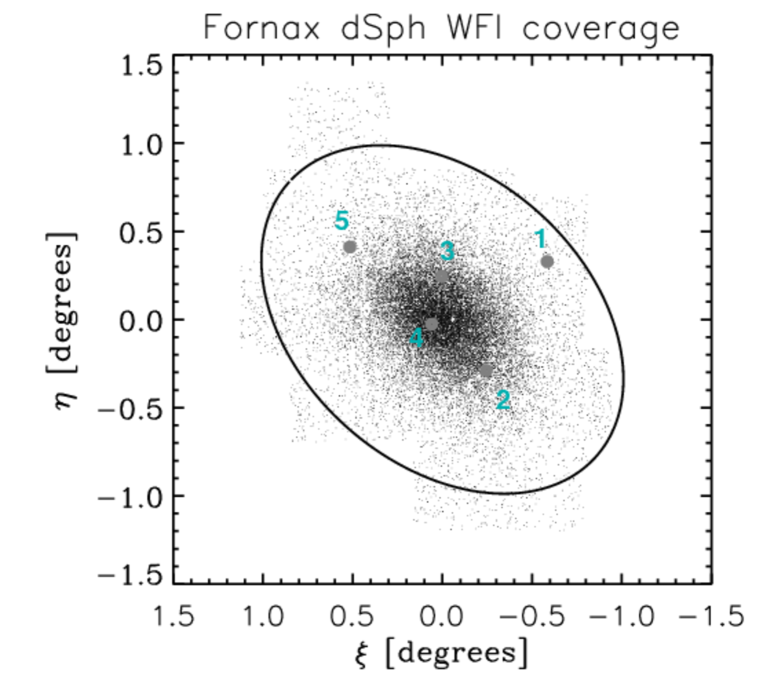
Figure 1: ESO/WFI coverage for Fornax dSph. The inner shell-like feature detected by Coleman et al. (2004) is located at $\xi\sim$0.12, $\eta\sim-$0.20 and elliptical radius of 0.33 deg. The circles indicate the location of Fornax globular clusters and the ellipse shows Fornax tidal radius (ellipse parameters derived in this work, see Table 1). The North is at the top, the East on the left-hand side. The physical scale at the distance of the Fornax dSph is 1 deg $=$ 2.4 kpc.

In this section we present the results of our wide field, ESO/WFI photometry of Fornax, out to its nominal tidal radius (see Fig.1), and going down to $V=$ 23 and $I=$ 22 (M${}_{\rm I}=$ 1.2).

3.1 The structure of Fornax

Previous studies have revealed the spatial structure of Fornax to be far from regular. Hodge (1961), using photographic plates, found that the ellipticity (defined as $e=1-b/a$, where $b$ and $a$ are respectively the semi-minor and major axes of the galaxy) increases with radius, from a value of 0.21 in the central regions to 0.36 in the outer parts. Irwin & Hatzidimitriou (1995) noticed that in the inner regions the isopleths showed departures from elliptical symmetry and that they were more closely spaced on the east side of the major axis than in the west, as already noticed by Hodge (1961). The asymmetry was found to be centred close to cluster 4 ($\xi\sim 0.05$, $\eta\sim-0.1$ in Fig. 1). The ellipticity was again found to increase with radius. Coleman et al. (2005), using only RGB stars, found that the position of the centre shifts 3^′ towards west within a radius of 20^′ and 4^′ towards south at all radii. For radii larger than 35^′ they find an opposite trend for the ellipticity, i.e. the outer contours become more circular.

Due to the variety of previous estimates, sometimes differing significantly from each other, we decided to re-derive the structural parameters of Fornax dSph. We divided the 2D spatial distribution of the stellar objects in our photometry (Fig. 1) into a grid with a “pixel” width of 0.02 deg and associated to each pixel the number of stars it contained. We then used the IRAF task ELLIPSE to derive the variation with radius of the central position, ellipticity and position angle (Fig. 2), by fitting ellipses at radii between 15^′ and 60^′ with a $\sim 5^{\prime}$ spacing. We find that the centre is at ($\alpha_{\rm J2000}$, $\delta_{\rm J2000}$) $=$ ($2^{h}39^{m}52^{s}$, $-34^{\circ}30^{\prime}49^{\prime\prime}$), west ($-1.5^{\prime}\pm 0.3^{\prime}$) and south ($-3.8^{\prime}\pm 0.2^{\prime}$) with respect to the values listed in Mateo (1998). The centre now appears to be located very close to cluster 4. With this new analysis the ellipticity, average value 0.30$\pm$0.01, does not show any trend with radius. The position angle (P.A.) appears to be larger in the inner 15^′ and then to become approximately constant with radius. A larger position angle for the inner region could be caused, for example, by the presence of cluster 4 or, more likely, by the presence of young stars with a markedly different distribution (see Sect. 3.3). In our subsequent analysis we adopt the average value of the P.A. to be 46.8${}^{\circ}\pm 1.6^{\circ}$, consistent with previous estimates. Our re-derived structural parameters are listed in Table 1. With the exception of the position of the centre of the galaxy, all the derived parameters are consistent with the values listed by Mateo (1998).

We also rederived the surface density profile for Fornax in bins of 3^′ out to a radius of 83^′ (see Fig. 3). The contamination by field star density, from a weighted average of the points beyond 68^′, is 0.78$\pm$0.02 stars arcmin^-2. From previous estimates of the tidal radius (e.g. Irwin & Hatzidimitriou 1995) we know that it is unlikely that our data extend out to a pure background region thus our determination of the Galactic contamination is of necessity an overestimate due to our limited spatial coverage. We compared this Galactic contamination subtracted profile to several surface brightness models using a least-square fit to the data. We used an empirical King profile (King 1962), an exponential profile, a Sersic profile (Sersic 1968) and a Plummer model (Plummer 1911).

The King model has been extensively used to describe the surface density profile of dSphs.

$$I_{\rm K}(R)=I_{\rm 0,K}\ \left(\frac{1}{\sqrt{1+\left(\frac{R}{r_{c}}\right)^{2}}}-\frac{1}{\sqrt{1+\left(\frac{r_{t}}{r_{c}}\right)^{2}}}\right)^{2}$$ (1)

It is defined by 3 parameters: a characteristic surface density, $I_{\rm 0,K}$, core radius, $r_{\rm c}$ and tidal radius, $r_{\rm t}$. The last parameter is defined as the distance, along the line connecting the galaxy centre and the centre of the host galaxy, where at the perigalacticon passage a star is pulled neither in nor out. This radius is set by the tidal field of the host galaxy. Thus, an excess of stars in the outer parts of dSphs with respect to King models have been interpreted as tidally stripped stars, assuming that the King profile is the correct representation of the data. Excess stars beyond the King tidal radius have been found in Fornax (e.g. Coleman et al. 2005) and in a number of other Local Group dSphs, e.g. Carina (Majewski et al. 2005), Draco (Wilkinson et al. 2004; Muñoz et al. 2005).

Another possibility to explain the excess of stars in the outer parts of dSphs is that the King model does not provide the best representation of the data at large radii. The Sersic profile is known to provide a good empirical formula to fit the projected light distribution of elliptical galaxies and the bulges of spiral galaxies (e.g. Caon et al. 1993; Caldwell 1999; Graham & Guzmán 2003; Trujillo et al. 2004):

$$I_{\rm S}(R)=I_{\rm 0,S}\ exp\left[-\left(\frac{R}{R_{\rm S}}\right)^{1/m}\right]$$ (2)

where $I_{\rm 0,S}$ is the central surface density, $R_{\rm S}$ is a scale radius and $m$ is the surface density profile shape parameter. The de Vaucouleurs law and exponential are recovered with $m=4$ and $m=1$, respectively; for $m<1$ the profile is steeper than an exponential; $m=1/2$ gives a Gaussian. The light profile of some dSphs in the Local Group are found to be best-fitted with $m<1$ (e.g. Caldwell 1999). Physical justifications for this law have been proposed (see for instance Graham & Guzmán 2003, and references therein), however none is widely accepted.

In our analysis King and Sersic profiles reproduce the data much better than a Plummer or an exponential profile. Our best fit is a Sersic profile with Sersic radius, $R_{\rm S}=$ 17.3$\pm$ 0.2 arcmin, and $m=$ 0.71, thus steeper than an exponential (Fig. 3).

For the best-fitting King model we find a core radius $r_{\rm c}=$ 17.5$\pm$0.2 arcmin and a tidal radius $r_{\rm t}=$ 69.4$\pm$0.4 arcmin. The core radius determined here is 4^′ larger than previous estimates whilst the tidal radius is in agreement with the value of 71$\pm$4 arcmin from IH95. The slightly smaller value we obtain for the tidal radius is likely due to our overestimated field star density.

Figure 3 shows that in our determination of the density profile there is an excess of stars with respect to the King profile (solid line) for radii larger than 1 deg. At this distance the Sersic profile (dashed) best follows the data. Both exponential and Plummer profiles (dotted and dash-dot) over-predict the surface density at $r<0.1$ deg and at radii larger than $\sim$ 0.8 deg, and under-predict it at intermediate distances. A summary of the best-fitting parameters is given in Table 2.

3.2 The Colour-Magnitude Diagram

It is well estabilished that the Fornax dSph has had a very complex star formation history (e.g. Stetson et al. 1998; Buonanno et al. 1999; Saviane et al. 2000). Stetson et al. (1998), in a photometric study covering a field of   1/3 deg² near the centre of Fornax, found that the majority of stars fall into three distinct stellar populations: an old one represented by HB and RR Lyrae stars; an intermediate age population of He-core-burning clump stars (Red Clump, RC); and a young population, indicated by the presence of main sequence stars. Fornax displays a broad RGB, classically interpreted as due to a large spread in metallicity.

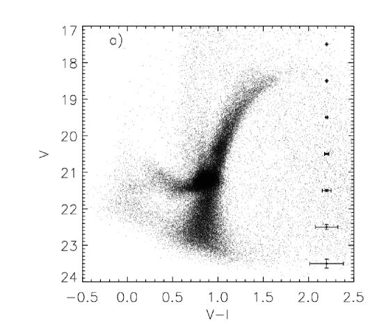
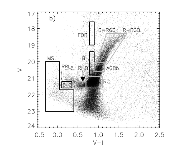
Figure 4: CMD for objects classified as stellar from our ESO/WFI imaging covering the whole extent of the Fornax dSph. The boxes in panel b) indicate the regions we used to select different stellar populations (MS: main sequence; BL: Blue Loop; FOR: foreground; BHB: Blue Horizontal Branch; RRLy: RRLyrae; RHB: Red Horizontal Branch; B-RGB: Blue-Red Giant Branch; R-RGB: Red-Red Giant Branch; AGBb: AGB bump; RC: Red Clump).

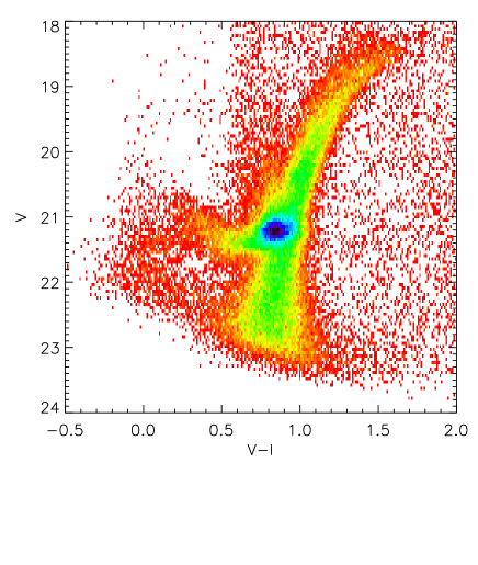
Figure 5: Here we show the Hess diagram for Fornax dSph CMD from ESO/WFI imaging, where the structures, and their relative intensity, in the different regions of the CMD are visible. Each cell is $\Delta(V-I)\times\Delta V=0.01\times 0.05$. A darker tone represents an higher density of stars; zero-density is set to white. This allows us to see the structure in the Red Clump and Red Horizontal Branch.

Figure 4a shows our WFI Colour-Magnitude diagram for Fornax within the tidal radius ($\sim 2^{\circ}\times 2^{\circ}$); it contains 73700 stars, including a quantity of foreground stars, which lie in a fairly constant density sheet redwards of $V-I=$ 0.6. We notice the following features (highlighted in Fig. 4b, and directly visible in the Hess diagram in Fig. 5):

3.2.1 Ancient stars ($>$ 10 Gyr):

These stars are to be found in:

• A red horizontal branch (RHB), extending from $V\sim$21.2 to $V\sim$21.6 and from $V-I\sim$0.5 to $V-I\sim$0.7. Hints of a blue horizontal branch (BHB) from $V\sim$21.2 to $V\sim$21.6 and from $V-I\sim$0.05 to $V-I\sim$0.35. Between the BHB and RHB we can see the instability strip where RR Lyrae variable stars are to be found.

• A broad Red Giant Branch (RGB) with distinct blue (B-RGB) and red (R-RGB) components. The RGB branch contain stars with ages $>$ 10 Gyr, as well as intermediate age stars (2-8 Gyr), as will be discussed in Sect.4.2. There is a hint of bifurcation below the tip of the RGB.

3.2.2 Intermediate age stars (2-8 Gyr):

These stars are to be found in:

• An “AGB bump”, from $V\sim$ 20.05 to $V\sim$ 20.6 and from $V-I\sim$0.9 to $V-I\sim$1.15. A similar feature was detected by Gallart (1998) in the LMC and called an “AGB bump”, and assumed to occur at the beginning of the AGB phase.

• A red clump (RC), that hosts the bulk of detected stars ($\sim 30$%) in our WFI CMD. It extends from $V\sim$ 20.9 to $V\sim$ 21.6 and from $V-I\sim$0.7 to $V-I\sim$1.1. From theoretical modelling of RC stars, Caputo et al. (1995) found that it is possible to estimate the age of the dominant stellar component from the extension in luminosity of the RC. They found that the larger the spread in luminosity the younger is the RC population. The predictions in Caputo et al. (1995) are made using models of metallicity Z=0.0001 and 0.0004, which is lower than the bulk of Fornax population (Z$\sim$ 0.002). Assuming a distance to Fornax of 138 kpc, an extinction in $V$ band of 0.062 (Schlegel et al. 1998) and a colour excess E($V-I$)$\simeq$0.026 the upper and lower $M_{\rm V}$ of the RC are 0.14 and 0.84. Using the above mentioned models, this translates into an age of 3-4 Gyr for the dominant stellar population, assuming no strong variation due to metallicity. We also derive the age of the dominant RC stellar population by overlaying to the observed CMD Padua isochrones (Girardi et al. 2000), which have a mass grid fine enough to resolve the red clump structure. Even though isochrones predictions for colour and magnitude of the red clump feature are valid for single stellar populations, they will provide a reasonably accurate estimate of the mean age of a composite stellar population such as Fornax. We find that the observed mean magnitude of the RC feature ($V=$ 21.2, see Fig. 5) is reproduced assuming a dominant stellar population of 2-4 Gyr old and metallicity Z in the range 0.001-0.004.

3.2.3 Young stars ($<$ 1 Gyr):

These stars are found in:

• A plume of young Blue Loop (BL) stars from $V\sim$ 19.4 to $V\sim$ 20.8 and from $V-I\sim$0.78 to $V-I\sim$ 0.9. Blue Loop stars are produced during the He-core burning phase for stars with mass $\gtrsim$ 2-3 $M_{\odot}$ and ages from few million years to 1 Gyr. The position (colour) of this feature is strongly dependent on metallicity (e.g. Girardi et al. 2000) .

• A main sequence extending from $V\sim$ 20 to $V\sim$ 23 at $V-I$$\sim 0$, showing that very recent star formation (less than 1 Gyr ago) has occurred in Fornax. The maximum luminosity of this feature indicates that there are stars as young as 200-300 Myr in Fornax.

3.3 The spatial distribution of different stellar populations

The spatial distribution of different stellar components in a galaxy gives an indication of how and where the star formation took place at different times and how long the gas was retained as a function of radius.

Previous studies of dSphs in the Local Group (e.g. Hurley-Keller et al. 1999; Majewski et al. 1999; Harbeck et al. 2001; Tolstoy et al. 2004) have shown that HB properties vary as a function of the distance from the centre in several dSphs: in general the RHB is more centrally concentrated than the BHB. This indicates the dominance of old and/or metal poor stars in the outer regions and younger and/or more metal rich stars in the inner regions.

Fornax contains both old (e.g. HB), intermediate (e.g. RC), and young stellar components (MS and Blue Loop stars). Previous photometric studies of individual stars, which have been limited to the central regions of Fornax dSph, have found indications that the intermediate age stars have a more concentrated distribution than the ancient stars (Stetson et al. 1998; Saviane et al. 2000). Stetson et al. (1998) found that the MS stars displayed a centrally concentrated asymmetric distribution, with a major axis tilted $\sim$ 30^∘ with respect to the main body of Fornax.

Our WFI data, covering the entire extent of Fornax, allow us to analyse the spatial distribution of the resolved stellar population of Fornax out to its nominal tidal radius. We plot a CMD for 3 different spatial samples, i.e. for stars found at elliptical radius $r<$ 0.4 deg, 0.4 deg $<r<$ 0.7 deg, and $r>$ 0.7 deg (Fig.6). Clear differences are visible between the inner and the outer regions: the main sequence and Blue Loop stars (young) are absent in the outer regions. The extent in $M_{\rm V}$ of the RC decreases with the distance to Fornax centre; this means that the age of the dominant stellar component in this feature is older in the outer parts (Caputo et al. 1995). We also notice that the BHB, which is almost hidden by the main sequence in the inner region, becomes more clearly visible the further out we go, because the MS disappears. Finally, we can see that the RGB changes: the red side, generally younger and more metal rich than the blue side, becomes less evident in the outer regions.

Below we analyse the spatial distribution of the different components, through their location in the field of view and the trend of the cumulative fraction with radius.

3.3.1 Ancient populations

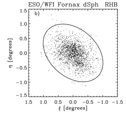
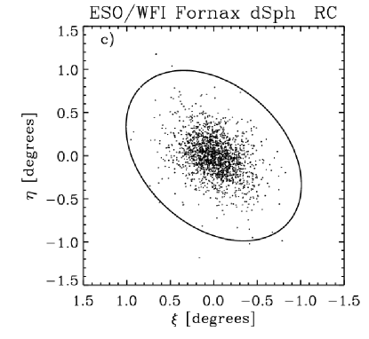
Figure 7: Spatial distribution of BHB, RHB and RC stars in the Fornax dSph as selected from the CMD shown in Fig. 4b. The RC stars show a more concentrated and less extended distribution than RHB and BHB stars. The number of RC stars has been normalised to the number of RHB stars.

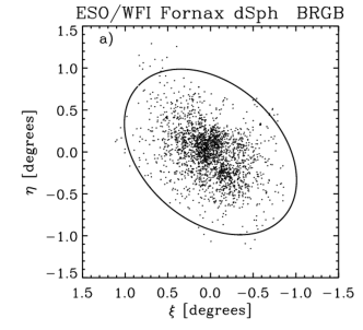
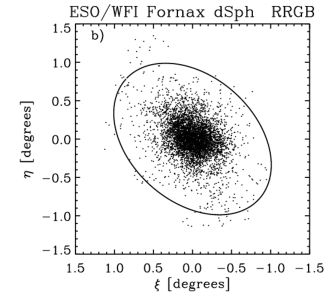
Figure 8: Spatial distribution of Blue RGB and Red RGB stars in the Fornax dSph (as selected from the CMD shown in Fig. 4b).

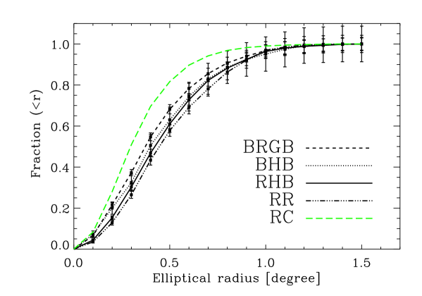
Figure 9: Surface number density (top) and fraction of stars within elliptical radius $r$ (bottom) of ancient stellar populations in the Fornax dSph (solid line: RHB stars; dotted line: BHB stars; dash-dot-dot line: RRLyrae stars; dashed line: B-RGB stars). The surface number density has been Galactic stellar contamination subtracted. Note that all the ancient stars, even if found at different stages of stellar evolution, display a similar spatial trend with radius. In the bottom panel we show for comparison the fraction of stars within elliptical radius $r$ for RC stars (long dashed line), representative of intermediate age stars: note the more extended and less concentrated spatial distribution of ancient stars with respect to intermediate age stars.

In Fornax the BHB stars overlap the MS in the inner regions, thus we reduce the selection box of BHB stars to V$-$I$\sim$0.15 - V$-$I$\sim$0.35. In Fig. 7a-b we plot the spatial distribution of the BHB and RHB components, and in Fig. 8a the location of B-RGB stars. Figure 9 shows the Galactic contamination subtracted density profile for the ancient populations (top) and the fraction of stars within a radius $r$, $f(<r)$, in bins of 0.1 deg (bottom). The ancient stellar components clearly all have the same distribution, the only exception being the trend at $r<$0.3 deg for the BHB population, which suffers from small number statistics. It is also likely that the BHB behaviour is altered by the presence in the selection box of MS stars (see Fig. 4b). A $\chi^{2}$ two-sample test applied to the percentage of stars within a radius $r$ out to the estimated Fornax tidal radius gives a probability of 99.99% that the ancient stellar populations are drawn from the same distribution.

Taking as reference the RHB cumulative distribution, we can see that 95% of the ancient population is found within $r\lesssim$ 0.9 deg. The dominant, intermediate age, stellar population in Fornax, i.e. RC stars, shows a distinctly different distribution, with 95% of its stars distributed within $r\lesssim$ 0.7 deg. Clearly, the ancient populations display a more extended spatial distribution then the intermediate age stars. The same $\chi^{2}$ test applied to the RHB and RC stars gives a low probability, 5%, that these two populations are drawn from the same parent population, confirming the fact that intermediate and ancient stars show very different spatial distributions.

There is evidence for small scale spatial substructure in part of the ancient stellar component of Fornax. In Fig. 8a (B-RGB) there is a clear overdensity of stars at $\xi\sim-0.15$ and $\eta\sim-0.25$ ($\alpha\sim 2^{h}39^{m}8^{s}$, $\delta\sim-34^{\circ}45^{{}^{\prime}}51^{``}$); this also appears to be present, though less pronounced, in the spatial distribution of RHB stars at similar position, however in contrast the distributions of BHB and RRLyrae stars appear to be smooth. We find the number of B-RGB within 4^′ of the above feature significantly larger (within 2$\sigma$) with respect to the number within 3 control fields, of the same dimensions and at the same elliptical radius; the overdensity of RHB is instead not statistically significant. A CMD centred on this overdensity shows a slightly bluer colour for the RGB in the over-density than in 3 control fields.

There is no evidence that the nearby cluster 2 ($\xi\sim-0.23$, $\eta\sim-0.30$ in Fig. 1) is related to this over-density, because the stars in the over-density do not match the cluster 2 CMD (e.g. Buonanno et al. 1998).

Similar overdensities in the stellar distribution have been found in previous works both in other dSphs as well as in Fornax dSph (e.g. Coleman et al. 2004).

3.3.2 Intermediate age populations

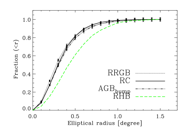
Figure 10: As in Fig. 9 but for intermediate age stellar populations (solid line: RC stars; dotted line: R-RGB stars; dash-dot-dot line: AGB bump stars). All the intermediate age populations display a similar spatial trend with radius. In the bottom panel we show for comparison the fraction of stars within elliptical radius $r$ for RHB stars (long dashed line), representative of ancient stars, as in Fig. 9: note the more extended and less concentrated spatial distribution of ancient stars with respect to intermediate age stars.

The spatial distribution of the intermediate age populations (2-8 Gyr old) is represented by RC, AGB bump and R-RGB stars distribution. Figure 7c shows the location on the field of view of the selected RC stars. As already mentioned, the RC stars form the dominant stellar population in Fornax. Thus, to allow a more meaningful comparison between the spatial distributions of intermediate age and ancient stars, we normalised the RC population to the number of stars present in the RHB. Visual comparison of these two distributions shows that RC stars have a less extended and more concentrated spatial distribution than RHB stars. The distribution of R-RGB stars (Fig. 8b) is similar to the RC stars, indicating a similar origin and thus similar age/metallicity properties for the stars found in the red part of the RGB in Fornax and in the RC. Figure 10 shows the Galactic contamination subtracted density profile (top) and the cumulative fraction (bottom) of RC, AGB bump and R-RGB: they clearly have the same spatial distribution; a $\chi^{2}$ test applied to the percentage of stars within a radius $r$ out to the estimated Fornax tidal radius gives a probability of 99.99% that the intermediate age stellar populations are drawn from the same distribution. Thus, it appears likely that all the stars with ages of 2-8 Gyr formed from the same gas distribution.

3.3.3 Young populations

We have already seen from the CMDs in Fig. 6 that young MS ($<$ 1 Gyr old) and BL stars are only present within $r<$ 0.4 deg, in the central region of Fornax. Figure 11 shows the spatial distribution of MS and Blue Loop stars (panel a,b). The main sequence stars are centrally concentrated and show a different, asymmetric distribution with respect to the older stars. They predominantly form a structure extended in the E-W direction, with a major axis tilted at $\sim 40^{\circ}$ with respect to the bulk of the stellar population (as already noted by Stetson et al. 1998). The overall spatial distribution of BL stars is also asymmetric, although not as pronounced as the MS. It is difficult to remove the effects of the foreground contamination (Fig. 11c) but it appears that the blue loop stars have a more relaxed distribution than the MS.

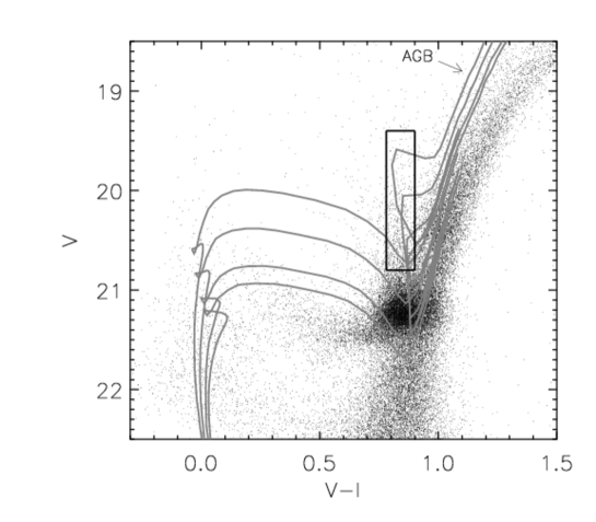
Figure 12: CMD for stars within 0.4 degree of the centre of the Fornax dSph; the box shows the selection region for the Blue Loop stars. The colours and magnitudes of the Blue Loop stars are consistent with theoretical Padua isochrones (Girardi et al. 2000) of metallicity Z=0.004 ([Fe/H]$\sim-$0.7) and age 0.4,0.5,0.6, 0.7 Gyr (from top to bottom). The stars forming the BL feature have mass in the range 2.3- 2.8 $M_{\odot}$ .

As mentioned in Sect. 3.2.3 the colour of the BL feature is strongly dependent on metallicity. Overlaying Padua stellar isochrones (Girardi et al. 2000) on the CMD (Fig. 12), we find that the Blue Loop stars are consistent with ages between 400 and 700 Myr and metallicity Z=0.004. Isochrones of lower metallicities (Z=0.001) predict the presence of a plume of Blue Loop giants much closer to the MS than observed, and the predicted average colour of the BL feature for higher metallicities (Z=0.008) is significantly redder than observed.

Figure 12 also shows that the Girardi et al. (2000) Padua isochrones suggest that the MS contains stars as young as 200-300 Myr, and as old as 1 Gyr, which is different with respect to the BL stars age range. Thus, to compare the spatial distribution of MS and BL stars, we must separate the MS stars in two groups, those predominantly younger and those older than 400 Myr. This is achieved by splitting the MS in colour: the “young” and “old” MS stars are approximately bluer and redder, respectively, than $V-I=$0. In this case we find that the spatial distribution of “old” MS stars is consistent with the BL spatial distribution, whilst “young” MS stars display a more asymmetric and centrally concentrated distribution. Thus, it seems that the “young” MS stars are found closer to the location where they were formed, whilst “old” MS and BL stars have diffused to larger radii. To estimate the diffusion time, we use the dynamical time (Binney & Tremaine 1987), which ranges between 350- 800 Myr, assuming a mass within the tidal radius between 10⁸-1.55$\times 10^{7}$ $M_{\odot}$ . This is consistent with the age of the “old” MS stars. Thus the elongated structure of the MS is formed predominantly by the younger MS stars, and is presumably the remaining signature of the collapsed gas from which the stars were formed.

3.3.4 A quantitative comparison between stellar populations

We have shown that the younger the stellar population the more concentrated and less extended is its spatial distribution over all the observed populations. We have also shown that stars in the same age range (but different stellar evolutionary phases) display very similar spatial distributions, and that the blue and red side of the RGB are linked to the ancient and intermediate age populations, respectively. A $\chi^{2}$ test is applied to the percentage of stars within a radius $r$ out to the estimated Fornax tidal radius for the several stellar components (Figs. 9, 10) gives a probability of 99.99% that RC, AGB and R-RGB stars are drawn from the same distribution, and again 99.99% for the different ancient stellar populations, whilst when comparing the distribution of an ancient population, e.g. RHB, to one of the intermediate age population, e.g. RC, we obtain a probability of 5% that they are drawn from the same spatial distribution. This shows that we can consider stars found at different stages of stellar evolution but with similar ages as belonging to the same population.

We derived density profiles, from which Galactic contamination has been subtracted, for these two components and compared them to the models used in Sec. 3.1.The best-fitting profile for the old population is given by the King model, that follows more closely the data beyond 1 deg with respect to the Sersic profile. However, the density profile of the intermediate age stars is better represented by a Sersic profile, since the King model declines too steeply. In both cases the exponential and Plummer models overpredict the density for $r\lesssim$ 0.2 deg and $r\gtrsim$ 0.9 deg, and underpredict it at intermediate radii. Independently from the adopted model, the results of the fit (see Table 2) show that intermediate age stars are more centrally concentrated and less extended than old stars.

The spatial distribution of different stellar populations is a powerful way to identify stellar populations of different ages in a dwarf galaxy.

3.4 Shells

The discovery of two shell-like features was recently reported in Fornax from photometric studies (Coleman et al. 2004, 2005). The first of these features was identified outside the core radius at $\alpha=2^{h}40^{m}28.5^{s}$ and $\delta=-34^{\circ}42^{\prime}33^{\prime\prime}$ (corresponding to $\xi\sim$0.12, $\eta\sim-$0.20 and elliptical radius of 0.33 deg in Fig. 1) as a small over-density of stars in data down to $I\sim$21 (Coleman et al. 2004). Adding deeper data from Stetson et al. (1998) to their sample the authors found the shell to be consistent with being dominated by young, 2 Gyr old, ZAMS stars. The authors proposed that this might be analogous to the shells found in elliptical galaxies and suggested that Fornax might have accreted a smaller gas-rich galaxy around 2 Gyr ago.

A second “shell” was found in the RGB distribution outside the tidal radius, around 1.3^∘ northwest from the centre (Coleman et al. 2005) and, similarly to the inner shell, located along the minor axis and elongated along the major axis.

Olszewski et al. (2006) carried out much deeper imaging of this over-density, down to $R\sim$ 26 and refined the age of the “feature” and suggested that the excess of stars in the shell might be the result of a burst of star formation which occurred 1.4 Gyr ago with a metallicity Z=0.004 ([Fe/H]$=-$0.7), favouring a scenario in which the gas from which these stars formed was pre-enriched within Fornax itself.

Our photometry covers the region of the inner shell, and we do not detect such a feature, but comparing our sample with the additional data-set from Stetson et al. (1998), we find signs of the shell when we include the stars we had discarded from our analysis because they were detected in $V$ but not in the $I$ band. This makes it clear that the feature is just at the detection limit of our data. We also note that the MS stars are asymmetrically distributed, and this could cause the presence of local overdensities with respect to other regions in Fornax, at the same elliptical radius, where young stars might be under-represented. Deeper photometry covering the entire region at $r<$0.4-0.5 deg would make it possible to resolve this issue.

4 Results: Spectroscopy

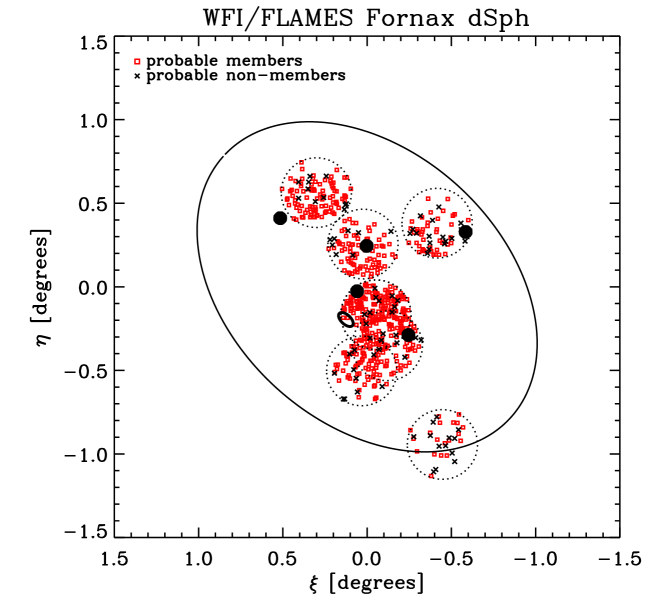
Figure 13: Location of the observed FLAMES fields and targets (with S/N per Å $>$ 10 and error in velocity $<$ 5 km s^-1 ) in the Fornax dSph (squares: probable members; crosses: probable non-members). The black filled circles show the location of Fornax globular clusters, the black small ellipse shows the location of the “shell-like” feature detected by Coleman et al. 2004, and the dashed circles indicate the observed FLAMES fields. The tidal radius is from this work.

Our VLT/FLAMES spectroscopic survey of individual stars in the Fornax dSph allows us to determine velocities and metallicities ([Fe/H]) from the CaT equivalent width for a subsample of RGB stars out to the nominal tidal radius of Fornax dSph (see Fig. 13).

The dependence of CaT equivalent width on metallicity has been empirically proven by extensive work in the literature (e.g. Armandroff & Zinn 1988; Olszewski et al. 1991; Armandroff & Da Costa 1991). Rutledge et al. (1997a) presented the largest compilation of CaT EW measurements for individual RGB stars in globular clusters, which Rutledge et al. (1997b) calibrated with high resolution metallicities, proving the CaT method to be reliable and accurate in the probed metallicity range, $-2.2<$[Fe/H]$<-0.6$.

We obtained metallicities from the CaT equivalent widths by using the relation derived by Rutledge et al. (1997b):

$${\rm[Fe/H]}=-2.66+0.42\,W^{\prime}$$ (3)

For deriving the reduced equivalenth width $W^{\prime}$ we used the equation below, as in Tolstoy et al. (2001):

$$W^{\prime}=(W_{\rm 8542}+W_{8662})+0.64(V-V_{\rm HB})$$ (4)

where $W_{\rm 8542}$ and $W_{8662}$ are the equivalenth width of the two strongest CaT lines, at $\lambda=8542.09$ Å and $\lambda=8662.14$ Å ; $V$ is the apparent $V$ magnitude of the star; and $V_{\rm HB}$ the mean magnitude of the horizontal branch. We checked this calibration against VLT/FLAMES HR measurements of an overlapping sample of 90 stars (Hill et al. 2006) to confirm our calibration and accuracy of CaT metallicity determination. Details will be provided in Battaglia et al. (2006b).

Since the Fornax dSph displays a very broad RGB (see Sect. 3.2 and Fig. 4) we chose our targets from a box around the RGB covering a wide colour range, to avoid biasing our sample in age or in metallicity. The spatial distribution of our targeted VLT/FLAMES is shown in Fig. 13, together with the position of Fornax globular clusters and the location of the shell-like feature (Coleman et al. 2004). The fields cover a wide range of radii. Since, as discussed in Sect. 3, the stellar population of different ages display different spatial distributions, our sample will contain predominantly intermediate age stars in the central fields, and ancient stars in the outermost fields. Previous studies, which were restricted to the central regions, were clearly biased towards the properties of the intermediate age population.

Figure 14 shows the velocity histogram of our VLT/FLAMES targets which met our S/N and velocity errors criteria (641 stars). To find the systemic velocity of Fornax we first selected the stars found within 4$\sigma$ of the velocity peak associated with Fornax. We used the value of $\sigma=$ 13 km s^-1 taken from the literature (e.g. Walker et al. 2005) as a first approximation. We calculated the mean velocity and the velocity dispersion from the 4$\sigma$ sample and then repeated the procedure selecting stars within 3$\sigma$ and finally the stars within 2.5 $\sigma$. We found a systemic velocity $V_{\rm sys}=53.1\pm$0.6 km s^-1 and a velocity dispersion $\sigma_{\rm los}=13.7\pm$0.4 km s^-1 (3$\sigma$), and $V_{\rm sys}=54.1\pm$0.5 km s^-1 , $\sigma_{\rm los}=11.4\pm$0.4 km s^-1 (2.5$\sigma$).

Because Fornax has a systemic velocity which strongly overlaps with the Galaxy, we tested to see if the large variation in velocity dispersion for different $\sigma$ cuts might be due to foreground contamination. We perform Monte Carlo simulations producing 10000 sets of 600 velocities about the mean velocity of Fornax Gaussianly distributed with a trial dispersion of 15 km s^-1 . The dispersions obtained cutting the artificial velocity set at 3 $\sigma$ and 2.5 $\sigma$ were consistent within 2 $\sigma$ in the 99.63% of the cases. We obtained very similar results when we fixed the dispersion at 12 km s^-1 , and/or convolved the simulated velocities with observational errors. This means that the differences in velocity dispersion we obtain with the $3\sigma$ and $2.5\sigma$ cuts for our data are most likely not due to the cuts themselves, but to the presence of Galactic contamination. A similar result is obtained by adding a Galactic component to the simulated velocities of Fornax, as a Gaussian with parameters determined from the Besançon model (Robin et al. 2003). The input velocity dispersion for the dSph velocity distribution is recovered with the $2.5\sigma$ cut, whilst the dispersion from the $3\sigma$ cut is overestimated. We thus adopt the 2.5$\sigma$ selection about the systemic velocity to limit the foreground contamination.

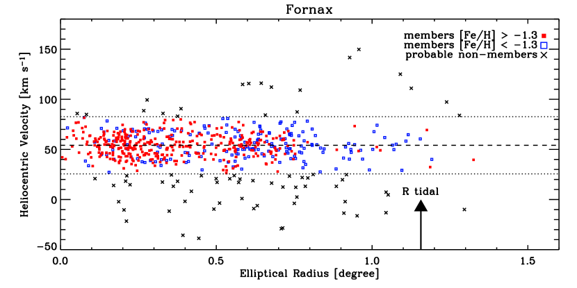
Figure 15: Heliocentric velocity with elliptical radius from VLT/FLAMES spectroscopic observations of individual RGB stars in the Fornax dSph. We plotted all the stars which satisfy our selection criteria (S/N per Å $>$ 10 and velocity error $<$ 5 km s^-1 ). The dashed line is the systemic velocity, $V_{\rm sys}=54.1$ km s^-1 , and the dotted lines encompass the 2.5$\sigma$ region of our kinematic selection. The squares show Fornax velocity members (filled: metal rich members, [Fe/H]$>-1.3$; open: metal poor members, [Fe/H]$>-1.3$), and the crosses foreground contamination.

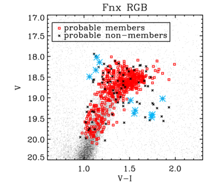
Figure 16: Location on the CMD of the observed FLAMES targets for Fornax dSph (squares: probable members; crosses: probable non-members). The boundaries of our target selection region closely follow the location of the targets. The asterisks indicates stars selected as velocity members falling in unusual position in the CMD; they are likely to be Galactic foreground contamination (see Fig. 17).

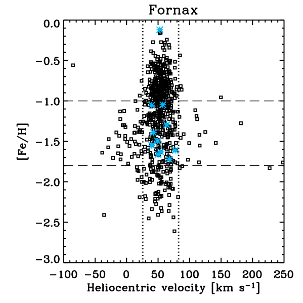
Figure 17: Metallicity versus heliocentric velocity for the observed FLAMES targets with S/N per Å  $>10$, and error in velocity $<$ 5 km s^-1 . The dotted lines show the region of our kinematic selection. Note that Galactic contaminants predominantly cluster between $-1.8<$[Fe/H]$<-1.0$ (horizontal lines). The asterisks show the Fornax velocity members present in unusual position in the CMD (see Fig. 16).

From our kinematic selection the number of probable Fornax members (with S/N per Å  $>$10 and error in velocity $<$ 5 km s^-1 ) is 562 (see Fig. 15). We list in Table 3 the relevant informations for the observed targets that passed our selection criteria. Note that probable members are also observed beyond the nominal tidal radius (derived in Sect. 3.1). In Fig. 16 we show the location on the CMD of probable velocity members and non-members. Because of the low heliocentric velocity of Fornax it is not always possible to firmly distinguish between members and non-members according to a pure kinematic selection: some members are present in a region of the CMD where none are expected. Visual inspection of these spectra shows that all but one are consistent with a RGB spectrum. However it is difficult to distinguish between dwarf and RGB stars in the spectral range covered by our data. The distribution of metallicity versus velocity (Fig. 17) shows that Fornax members are recognizable in this parameter space and the foreground stars (kinematic non-members) appear to cluster predominantly in the region between $-1.8<$ [Fe/H] $<-1$. The Fornax members off the RGB (asterisks in Fig. 16) are also identified in Fig. .17. All but one fall in the region between $-1.8<$ [Fe/H] $<-1$, thus the distribution of these stars in this parameter space again suggests that they are highly likely to be Galactic contamination. As the number of these objects is very small and removing or including them in our present analysis will not affect the conclusions, we decided to include them in the sample. A more strict membership selection will be carried out before analysing the detailed kinematics of Fornax (Battaglia et al. 2006a).

4.1 Chemo-dynamics

Several spectroscopic studies of individual stars in the Fornax dSph galaxy have shown that it is the most metal rich of the Milky Way dSph satellites (except for Sagittarius), with a peak metallicity at [Fe/H]$\sim-1.0$ and a large metallicity spread (Tolstoy et al. 2001; Pont et al. 2004). The extent of the metal poor and metal rich tail has changed depending mainly on the size and the spatial location of the observations. The most recent study, consisting of CaII triplet measurements of 117 RGB stars (Pont et al. 2004), showed that Fornax contains stars as metal poor as [Fe/H]$\sim-2.0$ and as metal rich as $-0.4$ with a peak at [Fe/H]$=-0.9$.

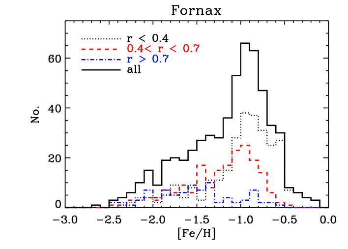
Figure 19: Histogram of metallicity measurements for individual RGB stars in the Fornax dSph (solid line: all velocity members; dotted line: velocity members within $r<$ 0.4 deg from the centre; dashed line: velocity members between 0.4$<r<$0.7 deg from the centre; dashed-dotted line: velocity members at $r>$0.7 deg from the centre).

Figure 18 shows the metallicity distribution with elliptical radius for the Fornax members kinematically selected from our VLT/FLAMES data. A variation of metallicity with elliptical radius is clearly visible: a metal poor population ($-2.8<$ [Fe/H] $<-1.2$) is seen throughout the galaxy; a more metal rich population ([Fe/H]${}_{\rm peak}\sim-$0.9) is present out to 0.7 deg from the centre; and an even more metal rich tail, extending out to [Fe/H]$=-$0.1, is present mainly in the inner 0.3-0.4 deg. This is quantified as an histogram in Fig. 19, where the sample is divided into 3 spatial bins (inner $r<$0.4, middle $0.4<r<0.7$, and outer $r>$0.7 ) and we can see that the metal poor component, centred at [Fe/H]$\sim-$1.7, is present in each bin and is thus spread throughout the galaxy; another component, centred at [Fe/H]$=-$1, with width at half peak of about 0.3, is present in the middle and inner regions; and only the innermost region contains the most metal rich component.

Such a large sample of velocity and metallicity measurements, covering a much larger area than previous studies, gives us the possibility to explore the relationship between the kinematics and metallicity in this galaxy. We divided the metallicity distribution into two parts: stars more metal rich (MR) and more metal poor (MP) than [Fe/H]$=-$1.3. This value of the metallicity was chosen to try and minimise the overlap between the two metallicity components. However a slightly different cut (e.g. [Fe/H]$-$1.2 or $-$1.4) does not significantly change the conclusions of our analysis.

Figure 20 shows the velocity distributions for the two metallicity components in 3 different spatial bins (inner $r<$ 0.4 deg, middle 0.4 $<r<$ 0.7 deg, outer $r>$ 0.7 deg). The metal poor population exhibits a larger velocity dispersion than the metal rich population (see Table 4); furthermore, in the first bin the velocity distribution of the metal poor stars is far from being Gaussian: it is flat or even double peaked (with peaks between 37-42 km s^-1 and 67-72 km s^-1 ). Changing the binning in the histogram leaves the main features of the velocity distribution unchanged. Figure 21 shows the cumulative function of the MP stars at $r<0.4$ deg compared to the cumulative distribution for a Gaussian with the same mean velocity and dispersion as the metal rich component in the same distance bin. The two cumulative functions are very different, and this also shows that the cumulative function of the MP stars is similar to what is expected for a uniform distribution, with two peaks at $\sim$ 40 km s^-1 and $\sim$ 70 km s^-1 .

An issue is if the velocity distribution of MP stars in the first bin is artificially biased by our choice of the metallicity cut, namely if by assigning metal poor stars to the metal rich component we could cause the small observed number of MP stars with velocity close to the systemic in the inner bin. This can be explored by changing the cut in metallicity, e.g. using [Fe/H] $<-1.6$ for the metal poor component, and [Fe/H] $>-1.1$ for the metal rich one. We find the same features for the MP distribution at $r<$ 0.4 deg as in the case with a metallicity division at [Fe/H]$=-1.3$, showing that the choice of a different metallicity cut does not alter our conclusions and accentuates the differences between the velocity distributions for metal rich and metal poor stars.

We tested to see if the differences in velocity distribution between the metal poor and the metal rich components are statistically significant: can the metal poor population in the inner bin be drawn from the metal rich and how significant would this be? A two-sided KS-test applied to the velocity distributions gives a probability of 0.7%, 0.4% and 16% that the MP stars in the first bin might be drawn from the same distribution as respectively: the MR stars in the inner bin; the MR stars in the middle bin; the MP stars in the middle bin. Thus the differences in the velocity distribution of MR and MP stars are unlikely to be an artifact of the observed number of stars, and instead point to significantly different kinematic behaviour of different metallicity components.

We also tested to see if the differences between the velocity distribution of MP stars in the inner and middle bins, reflected in the relatively low value of the K-S test, are due to the peculiarities of the velocity distribution of the MP stars at $r<$ 0.4 deg, or are intrinsic. Thus, we artificially “removed” the two velocity peaks by considering as the “expected” number of stars at the velocities of the peaks as the average of the number of stars in the adjacent bins. We then randomly removed the stars in “excess” from the velocity peaks (5.5$\pm$2.3 for the peak at $\sim$ 40 km s^-1 and 14$\pm$4 at $\sim$ 70 km s^-1 ). The velocity distribution of the remaining stars is compatible with a Gaussian distribution with velocity dispersion $\sigma=13.4\pm 1.74$ km s^-1 (probability of 99.85% from a KS-test). In this case MP stars in the inner and middle distance bins have a 93.7% probability to have been drawn from the same velocity distribution.

Thus Fornax dSph shows clear differences in the kinematics of its MR and MP component. Contrary to expectations, part of the metal poor component, arguably the oldest component, displays non-equilibrium kinematic behaviour at $r<$ 0.4 deg. A possible explanation for this is that Fornax recently captured external material which is disturbing the underlying distribution. Since we detect signs of disturbance only in the MP component, we argue that part of the object accreted by Fornax must have been dominated by stars more metal poor than [Fe/H]$<-1.3$.

4.2 Age determination

It is well known that the main uncertainty in deriving the absolute ages of stars in a CMD of a complex stellar population (ie. a galaxy) is that the position of a star changes depending degenerately upon both age and metallicity. We can break this degeneracy using metallicities derived from spectroscopy. In Fornax we can use our spectroscopic metallicities of 562 RGB stars to determine which isochrone set to use to determine the ages of these stars, and thus produce an age-metallicity relation for the galaxy over the age range covered by RGB stars ($>$1Gyr). The ages we determine in this way remain uncertain in absolute terms due to the limitations in the stellar models used to create the isochrones, but in relative terms the ages are accurate. Given the low systemic velocity of Fornax there will be foreground stars contaminating our samples.

We chose to use the Yonsei-Yale isochrones (Yi et al. 2001; Kim et al. 2002) because they cover the range of ages and metallicities we require in a uniform way, and they allow for a variation in [$\alpha$/Fe]. They also provide a useful interpolation programme which allows us to efficiently calculate the exact set of isochrones to compare with each spectroscopic metallicity. These isochrones did have the problem that they did not always extend up to the tip of the RGB for young metal rich stars, but comparison with the Padua isochrones (Girardi et al. 2000) of the same metallicity suggested that we could extrapolate these Y-Y isochrones to the tip of the RGB which allowed us to determine ages of the young metal rich stars in our sample.

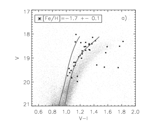
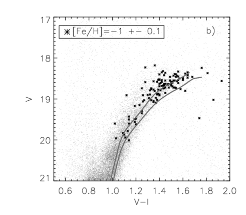
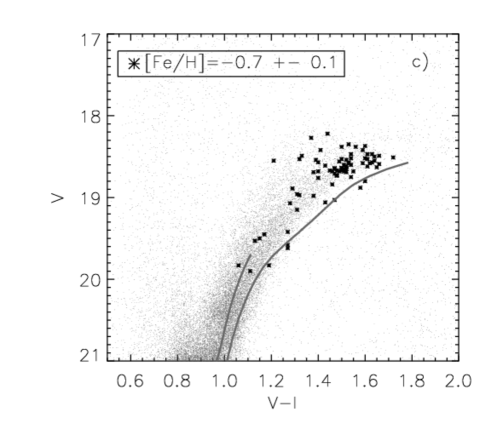
Figure 22: The comparison between measured metallicities and colours of Fornax stars (asterisks) with the theoretical isochrones (lines) for the metallicity of the stars. a) Stars with [Fe/H]$=-1.7\pm$0.1 and two YY isochrones of [Fe/H]$=-1.7$ and age 2 and 13 Gyr (from left to right). b) Stars with [Fe/H]$=-1\pm 0.1$ and two YY isochrones of [Fe/H]$=-1$ and age 2 and 5 Gyr (from left to right). c) Stars with [Fe/H]$=-0.7\pm$0.1 and two YY isochrones of [Fe/H]$=-0.7$ and age 1 and 2 Gyr (from left to right).

In Fig. 22a we plot the CMD of the 39 stars in our spectroscopic sample with [Fe/H]$=-1.7\pm 0.1$ and over-plot the Y-Y isochrones of the same metallicity for two different ages: the majority of metal poor stars fall on the blue side of the RGB and are consistent with old ages ($>$10Gyr old), and thus can be associated with the ancient component from the photometric analysis in Sect. 3. The stars found outside the range of the isochrones to the red ($V-I\gtrsim$ 1.4) may be Galactic contamination. There are also several quite blue stars (at $V-I\sim$ 1.1; $V\sim$ 18.3) which are consistent with having young ages (2 Gyr), and these are most likely to be foreground contamination. The more metal rich stars for which we have spectroscopy, with [Fe/H]$=-1\pm 0.1$ (119 stars), are shown in Fig. 22b. They are generally consistent with young, 2-5Gyr old, isochrones and match the dominant intermediate age component found in the photometric analysis. Fornax members at higher metallicity ([Fe/H]$=-0.7\pm 0.1$) are better represented by ages of 1.5 -2 Gyr (Fig. 22c).

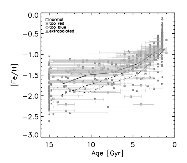
Figure 23: Ages and errorbars derived from isochrones fitting of the VLT/FLAMES spectroscopic sample of RGB stars in Fornax dSph. The lines shows the average value of [Fe/H] as a function of age assuming [$\alpha$/Fe]$=0$ (solid), [$\alpha$/Fe]$=0.3$ (dotted), and [$\alpha$/Fe] decreasing with [Fe/H] (dashed). The stars plotted as asterisks and diamonds were excluded from the analysis because they fell outside the age range of the isochrones for the considered metallicity.

In Fig. 23 we show the age-metallicity relation obtained for Fornax from fitting Y-Y isochrones to our entire spectroscopic sample. We used [$\alpha$/Fe]$=0$, in agreement with the average value from preliminary HR measurements of RGB stars in the centre of the Fornax dSph (Letarte et al. 2006b). We derived the errors in the age determination from the errors in magnitude and colour of the photometry, and assuming a metallicity error of 0.1 dex for each star. This figure contains 466 stars (out of the total sample of 562 stars), among which 103 were young stars which were too bright for the young isochrones (but fainter than the tip of the RGB); 97 stars fell completely outside the age range of the isochrones and therefore had to be excluded.

If we change the [$\alpha$/Fe] assumed, and repeat our age determination for [$\alpha$/Fe]$=$ 0.3; and for a variation in $\alpha$ with [Fe/H] ([$\alpha$/Fe]$=0.2$ for [Fe/H] $<-1.7$ and decreasing to [$\alpha$/Fe]$=0$ between [Fe/H] $=-1.7\&-1.0$ and then remaining constant), as found in HR studies of the central region of Fornax (Letarte et al. 2006b) we obtain slightly different results as shown by the relations plotted in Fig.  23. The different trend is enhanced by the fact that previously excluded groups of low metallicity stars when using [$\alpha$/Fe]$>0$ isochrones could now be included. Thus the $\alpha$-element abundance of a star has an impact on deriving accurate ages, and it would clearly be desirable to be able to correct for this effect for each star. Unfortunately [$\alpha$/Fe] determination requires HR spectroscopy and for the large sample here this is a daunting task. However we can make use of the HR study of the central region and use the general trends found there. HR studies (Letarte et al. 2006b) find that [$\alpha$/Fe]$<0$ for [Fe/H]$\gtrsim-1.0$, however as there are no currently available sets of isochrones for [$\alpha$/Fe]$<0$, it is not clear how this will affect our age estimates. Assuming the interpolation between [$\alpha$/Fe] = 0.3 and 0. continues to $-$0.3 this would go in the direction of reconciling the discrepancies between the observations and the isochrones at high metallicities.

5 Discussion

5.1 Age & Metallicity Gradients

One of the main results of our imaging and spectroscopic survey of the Fornax dwarf spheroidal galaxy is the presence of a population gradient. The stellar population shows a clear variation in age and metallicity as a function of radius (e.g. Figs. 6, 14 and 19). We can associate most of the more metal poor component with an ancient population ($>10$Gyr), and most of the more metal rich component with an intermediate age population (2-8 Gyr) with overlapping metallicity distributions.

Population gradients have been detected in several other dwarf spheroidal galaxies in the Local Group from imaging (e.g., Harbeck et al. 2001), and spectroscopy (e.g., Tolstoy et al. 2004). This must point to some common process in the formation of stars in these small systems, as this variation most likely reflects the original spatial distribution of gas from which the different stellar populations were formed. It is unlikely that the spatial distribution of one stellar component can have changed significantly with respect to another over time. Although weak encounters could diffuse an older component, it is unlikely to be an important effect because the relaxation time (Binney & Tremaine 1987) of Fornax is $>1.5\times 10^{10}$ years, i.e. longer than the age of the ancient population. Therefore, the present spatial distribution of stars of different ages gives us an indication of how the gas from which they were formed was distributed, and requires an explanation for how gas has apparently been progressively “removed” from the outer regions, and more recently, apparently, completely from the system.

Star formation is likely to have a dramatic impact on the interstellar medium of these small galaxies. It is possible that gas is frequently blown away as the result of supernovae type II explosions of massive stars (e.g. Mac Low & Ferrara 1999; Mori et al. 2002). This expelled gas should be able to fall back onto the galaxy, if the galaxy has a large enough potential, and on its return the gas will sink deeper into the central regions, where further generations of star formation can occur, with potentially different spatial, kinematic, metallicity and age characteristics. This next generation stellar population will likely be a more centrally concentrated, younger, more metal rich component. In this case we should expect a direct correlation between the mass of the galaxy and the fraction of gas retained by the system, as the deeper potential well of the most massive dSphs is more capable of retaining more of the original gas (e.g., Ferrara & Tolstoy 2000). Consistent with this picture, Fornax differs from the less massive Sculptor dSph in having a much more extended star formation history.

However this correlation is not a straight forward prediction of the properties of all the dwarf galaxies in the Local Group. This is because it is not only the mass of galaxies that determines their ability to retain an interstellar medium; dSph typically live in a fairly active environment with competing effects of the tidal field of our much larger Milky Way and several fairly large interacting companions (e.g., the Magellanic Clouds), and the debris left around by these interactions (e.g., the Magellanic Stream). N-body simulations indicate that tidal stripping combined with ram pressure stripping is a feasible combination to explain the lack of gas at the present time in dSphs (Mayer 2005). The importance of these effects depends strongly on the orbital parameters of the satellite, the apocenter-to-pericenter ratio, and the time at which the satellite enters the Milky Way potential. Whilst the satellite is orbiting the Galaxy, part of its gas may be ionized by the Milky Way corona, perhaps in combination with the cosmic UV background. The gas can be then removed over time, with varying degrees of efficiency, if the apocenter-to-pericenter ratio is large enough.

Recent proper motion measurements for Fornax suggest a pericentric distance of the order of the present Galactocentric distance (Piatek et al. 2002; Dinescu et al. 2004), and an almost circular orbit with an orbital period of $\sim$ 4-5 Gyr (Dinescu et al. 2004). Even though proper motion measurements are rather uncertain, this would suggest that we can exclude strong interaction with the Milky Way. Thus, as suggested by Mayer (2005), an object like Fornax may not be completely stripped of its gas, but would be able to retain it in its central regions and thus maintain an extended star formation history.

N-body models that predict dIrr to be the progenitors of dSphs, transformed into spheroids by tidal stirring from the Milky Way (Mayer et al. 2001a, b), predict an increase in the star formation activity of a satellite after pericentric passage. The pericentric passage can also provoke the formation of a bar that funnels gas into the central region, making the gas distribution more centrally concentrated. These models are highly dependent upon the starting conditions for the satellite. It is found that an apocentre-to-pericentre ratio of $\sim$ 5 and a pericentre distance of $\sim$ 50 kpc would be required to transform a dIrr into a dSph. Fornax has never been specifically modeled, however, as it is now thought to be close to its pericentre and the previous passage probably occurred around 4-5 Gyr ago, this would correspond well to the time frame of the last period of intense star formation. This scenario could explain both the variation in the spatial distribution of the Fornax stellar population and the large fraction of intermediate age stars. Specific simulations, emulating the orbital parameters of Fornax, are required for a more detailed comparison between these observations and N-body simulations.

5.2 Peculiar Kinematics

In addition to the different spatial distribution of ancient, intermediate age and young stars, we also find a different kinematic behaviour of metal rich and metal poor stars. This behaviour appears similar to what is seen, for example, in our Milky Way. The stellar bulge of our Galaxy is much less extended and kinematically colder than the stellar halo. This distinction may merely reflect the different spatial distribution required by a star moving with a larger velocity to reach larger distances or it may be telling us something more fundamental about the different conditions of the formation of these two different components. To test this we can use the Jeans equation to derive the line of sight velocity dispersion predicted for stars following the different density profiles of old and intermediate age stars (Binney & Tremaine 1987). This calculation shows that it is difficult to interpret the observed differences in velocity dispersion of MR and MP stars as being only due to their different spatial distribution (Battaglia et al. 2006a), and the same result is found in N-body simulations (e.g Kawata et al. 2006). In a future paper we will present detailed kinematic modelling of these distinct stellar populations, taking into account the possibility of different orbital properties for the two populations (Battaglia et al. 2006a).

Another aspect that deserves further investigation is the apparently non-equilibrium kinematics of the metal poor, presumably the oldest, stellar population in the center of Fornax. A possible interpretation of this is that we are seeing a remnant of accreted material. Given the presence of 5 globular clusters in Fornax, it would not be surprising for this to be a disrupted globular cluster. In this case we would expect the metallicity distribution of the stars forming the velocity feature to be extremely narrow, however the metallicity of the stars in the double peak ranges from $-2\lesssim$[Fe/H]$\lesssim-1.4$, showing a much larger spread than can be accounted for by a globular cluster.

An alternative explanation, as proposed by Coleman et al. (2004, 2005), is that Fornax accreted a smaller galaxy at some point in the recent past. These authors propose the accretion of a gas-rich dwarf $\sim$ 2 Gyr ago. In this case the MP stars with unrelaxed kinematics could be the remnant of the disrupted old stellar component of this accreted galaxy, and the asymmetric spatial distribution of the young stars (BL and MS) could be a result of the gas which subsequently formed stars as a consequence of the accretion process. Measuring the metallicities of the young stars in Fornax could help to answer this question by determining whether or not they are consistent with the bulk of the older stellar population in Fornax. Unfortunately we do not have spectroscopic metallicities of these stars, but the indications from the colour of the Blue Loops in the CMD (see section 3.3.3) suggest that these stars have a metallicity of [Fe/H]$\sim-0.85\pm 0.15$, consistent with the mean of the youngest RGB stars (age $>$1-2 Gyr) in our VLT/FLAMES sample. However, our FLAMES sample also contains a significant number of stars with higher metallicity, up to [Fe/H]$\sim-0.1$. Assuming we can directly compare metallicities derived with these two different methods, this could be an indication that Fornax has recently ($<$1-2 Gyr ago) been polluted with external gas of lower metallicity than the gas in Fornax at that time. This would also explain the peculiar kinematics of the MP stars in the centre of Fornax. However, this conclusion requires further confirmation, such as high resolution follow-up of the metal rich RGB stars in the central region (Letarte et al. 2006b), spectroscopic analysis of the Blue Loop and/or main sequence stars, and detailed dynamical modelling.

6 Summary

We have presented results from accurate ESO/WFI photometry of resolved stars in the Fornax dSph galaxy covering the entire extent out to its nominal tidal radius, and also velocity and metallicity measurements from our VLT/FLAMES spectroscopy of 562 RGB stars also out to the nominal tidal radius.

Using our ESO/WFI photometry we re-derive basic structural parameters of Fornax such as central position, ellipticity and position angle. In common with previous imaging studies we show that the Fornax dwarf spheroidal galaxy contains 3 stellar components: an ancient component, with ages between 10-15 Gyr old, which is spatially extended; an intermediate age component, with ages 2-8 Gyr old, that contains the bulk of the stellar population ($\sim$ 40%), which is more centrally concentrated and less extended with respect to the older component; a young population, with stars younger than $\sim$ 1 Gyr old. The youngest component ($<$1 Gyr old) is the most centrally concentrated and is completely absent beyond a radius of 0.4 deg from the centre, and it shows an asymmetric, disc-like (or bar-like) distribution. Within this component, the 200-300 Myr old stars show the most asymmetric and centrally concentrated distribution. The colour of the plume formed in the CMD by Blue Loop stars indicates that this young population has a metallicity [Fe/H] between $-0.7$ and $-1.0$. Spatial analysis shows that substructures might be present in the ancient stellar population represented by the B-RGB.

The VLT/FLAMES spectroscopy in the CaT wavelength region for a sample of 562 Fornax RGB velocity members shows that the mean metallicity of the stellar population changes with radius with the central regions more metal rich than the outer regions. No stars more metal poor than [Fe/H]$\lesssim-2.7$ are found anywhere in the galaxy, but we can distinguish a metal poor component, with a mean of [Fe/H]$\sim-1.7$ and extending from $-2.5\lesssim$[Fe/H]$\lesssim-1$, that is found throughout the galaxy; a more metal rich component, with a mean of [Fe/H]$\sim-1$ and extending from $-1.5\lesssim$[Fe/H]$\lesssim-0.5$, present mainly within 0.7 deg from the centre and is thus more spatially concentrated than the metal poor stars; a metal rich tail, [Fe/H]$\lesssim-0.1$, is found at radii less than 0.4 deg from the centre. “Metal rich” and “metal poor” populations (stars with [Fe/H]$>-1.3$ and $<-1.3$, respectively) show different kinematics: metal rich stars have a colder velocity dispersion than metal poor stars, and these differences are not dependent on the metallicity cut. The metal poor component shows signs of non-equilibrium kinematics in the inner regions ($r<0.4$ deg), arguably due to the accretion of external material. A more complete modelling of chemo-dynamics of Fornax is the subject of a future paper (Battaglia et al. 2006a).

[x]lccccc Table of Fornax ESO/WFI observations. The seeing is the average stellar FWHM from the final image.
Name Filter UT of observation airmass exptime seeing (arcsec)
continued.
Name Filter UT of observation airmass exptime seeing (arcsec)
FNX-1 V 07-Jan-2005 02:13 1.1 3x300s 0.87
I 1.1 3x300s 0.89
FNX-2 V 07-Jan-2005 02:55 1.2 3x300s 0.90
I 1.2 3x300s 0.80
FNX-3 V 07-Jan-2005 03:39 1.3 3x300s 0.93
I 1.3 3x300s 0.93
FNX-4 V 07-Jan-2005 04:22 1.5 3x300s 1.13
I 1.6 3x300s 0.87
FNX-13 V 08-Jan-2005 02:19 1.1 3x300s 0.75
I 1.1 3x300s 1.19
FNX-5 V 08-Jan-2005 02:55 1.2 3x300s 0.82
I 1.2 3x300s 1.12
FNX-6 V 08-Jan-2005 03:26 1.3 3x300s 1.03
I 1.3 3x300s 1.00

FNX-8 V 01-Feb-2005 01:54 1.3 3x300s 0.98
I 1.3 3x300s 0.94
FNX-9 V 01-Feb-2005 02:18 1.4 3x300s 1.09
I 1.5 3x300s 0.97
FNX-14 V 01-Feb-2005 02:54 1.6 3x300s 1.01
I 1.7 3x300s 0.93
FNX-16 V 02-Feb-2005 01:35 1.2 3x300s 1.09
I 1.3 3x300s 1.21
FNX-7 V 01-Feb-2005 01:16 1.2 3x300s 1.02
I 1.2 3x300s 0.97
FNX-21 V 03-Feb-2005 02:10 1.4 3x300s 1.02
I 1.5 3x300s 1.09

SA98 V 06-Jan-2005 05:08 1.2 10s,30s 0.92,0.95
I 05:19 1.2 10s,30s 0.93,0.94
SA95 V 07-Jan-2005 01:32 1.2 10s,30s 1.06,1.03
I 01:44 1.2 10s,30s 1.06,0.80
RU-149 V 07-Jan-2005 05:02 1.2 5s,30s 0.89,0.95
I 05:12 1.2 10s,30s 1.66,1.16
SA95 I 09-Jan-2005 02:48 1.2 10s,30s 1.16,1.26
RU-149 V 31-Jan-2005 00:46 1.0 5s,30s 3.55,3.61
I 01:00 1.0 10s,30s 2.70,2.56
SA98 V 01-Feb-2005 00:30 1.4 10s,30s 0.98,0.93
I 00:42 1.3 10s,30s 1.14,1.24
SA95 V 02-Feb-2005 00:44 1.2 10s,30s 1.24,1.22
I 00:58 1.2 10s,30s 1.05,1.02
SA101 V 02-Feb-2005 08:33 1.5 10s,30s 0.94,1.15
I 08:41 1.5 10s,30s 1.30,1.22
PG1323-086V 02-Feb-2005 09:10 1.1 5s,30s 0.86,0.91
I 09:22 1.1 10s,30s 1.20,1.07
SA95 V 03-Feb-2005 01:37 1.3 10s,30s 0.95,0.87
I 01:48 1.3 10s,30s 0.91,0.80
SA107 V 03-Feb-2005 09:17 1.4 10s,30s 0.79,0.88
I 09:28 1.3 10s,30s 0.69,0.74
SA98 V 04-Feb-2005 01:02 1.2 10s,30s 1.16,1.23
I 01:13 1.2 10s,30s 0.63,0.74

Table 1: Table of Fornax parameters. 1. This work. 2. Mateo et al. (1998). The position angle is defined as the angle between North and the major-axis of the galaxy measured counter-clockwise; the ellipticity is $e=1-b/a$.

$\alpha_{\rm 2000}$	$2^{h}39^{m}52^{s}$	1
$\delta_{\rm 2000}$	$-34^{\circ}30^{\prime}49^{\prime\prime}$	1
Position angle	$46.8^{\circ}\pm 1.6^{\circ}$	1
Ellipticity	$0.30\pm 0.01$	1
$L_{V}$	$1.55\times 10^{7}L_{\odot}$	2
Distance	$138\pm 8$ kpc	2
$V_{\rm h}$	$54.1\pm 0.5$ km s-1	1
${\rm[Fe/H]}_{\rm mean}$	$-1.15$	1

Table 2: Parameters of best-fitting King model (core radius, $r_{\rm c}$, tidal radius, $r_{\rm t}$), Sersic model (Sersic radius, $R_{\rm S}$, shape parameter, $m$), exponential model (scale radius, $r_{\rm s}$) and Plummer model (scale radius, $b$) for all stellar populations, intermediate age and old stellar components in Fornax dSph. For each model we also compute the half-number radius, $r_{\rm h}$; for the Plummer model this coincides with $b$. The errors in the parameters are formal errors from the fitting procedure.

	King			Sersic			Exponential		Plummer
	$r_{\rm c}[^{\prime}]$	$r_{\rm t}[^{\prime}]$	$r_{\rm K,h}[^{\prime}]$	$R_{\rm S}[^{\prime}]$	$m$	$r_{\rm S,h}[^{\prime}]$	$r_{\rm s}[^{\prime}]$	$r_{\rm Ex,h}[^{\prime}]$	$b[^{\prime}]$
All	17.6$\pm$0.2	69.1$\pm$0.4	19.1	17.3$\pm$0.2	0.71 $\pm$ 0.01	18.6	11.0$\pm$0.1	18.5	19.6$\pm$0.1
Intermediate	15.7$\pm$0.2	68.5$\pm$0.4	18.1	16.7$\pm$0.2	0.69 $\pm$ 0.01	17.5	10.0$\pm$0.1	16.7	17.1$\pm$0.1
Old	26.8$\pm$1.1	77.2$\pm$1.6	23.7	24.6$\pm$0.8	0.62 $\pm$ 0.02	23.5	13.7$\pm$0.2	23.0	24.6$\pm$0.4

Table 3: Data for the observed VLT/FLAMES targets in Fornax dSph. Column (1) ID; (2) $\alpha_{\rm J2000}$; (3) $\delta_{\rm J2000}$; (4) $V$ magnitude; (5) $\sigma_{V}$; (6) $I$ magnitude; (7) $\sigma_{I}$; (8) signal-to-noise ratio per Å ; (9) [Fe/H]; (10) $\sigma_{\rm[Fe/H]}$; (11) membership ID (Y= kinematic member; N= kinematic non-member). The errors in metallicity are based on S/N computations and adjusted to agree with repeated measurements.

ID

$\alpha_{\rm J2000}$

$\delta_{\rm J2000}$

$V$

$\sigma_{V}$

$I$

$\sigma_{I}$

S/N per Å

[Fe/H]

$\sigma_{\rm[Fe/H]}$

Member

Table 4: Number of stars, weighted mean heliocentric velocity, and line of sight velocity dispersion for Fornax members (all mem), metal rich (MR) and metal poor (MP) stars at every elliptical radius (all $r$), and in 3 distance bins ($r<0.4$, $0.4<r<0.7$, $r>0.7$ deg).

		all $r$		$r<0.4^{\circ}$		$0.4^{\circ}<r<0.7^{\circ}$		$r>0.7^{\circ}$
	all mem	MR	MP	MR	MP	MR	MP	MR	MP
number	562	377	185	232	53	122	68	23	64
$<V>$	54.1$\pm$ 0.5	53.9$\pm$0.6	54.5$\pm$1.0	53.3$\pm$ 0.8	57.7$\pm$ 1.9	54.5$\pm$ 0.9	53.1$\pm$ 1.5	54.8$\pm$ 1.9	53.0$\pm$ 1.7
$\sigma$	11.4$\pm$ 0.4	10.6$\pm$0.4	13.0$\pm$0.7	11.3$\pm$ 0.5	13.6$\pm$ 1.4	9.9$\pm$ 0.7	12.3$\pm$ 1.1	8.6$\pm$ 1.4	13.1$\pm$ 1.2

Figure 2: The variation with radius of the central position ($x$ and $y$ coordinate, a) and b) respectively), c) ellipticity and d) position angle for the entire stellar population of Fornax, from ESO/WFI imaging data. The variation of the central position is with respect to the value listed in Mateo (1998). We find that the centre is at $\alpha=2^{h}39^{m}52^{s}$ and $\delta=-34^{\circ}30^{\prime}49^{\prime\prime}$, west ($-1.5^{\prime}\pm 0.3^{\prime}$) and south ($-3.8^{\prime}\pm 0.2^{\prime}$) with respect to the values listed in Mateo (1998).

Figure 3: The surface density profile for Fornax dSph galaxy with overlaid best-fitting King, Sersic, exponential and Plummer models (solid, dashed, dotted, dash-dot lines, respectively). The Galactic stellar contamination, 0.78$\pm$0.02 stars arcmin^-2 calculated from a weighted average of the points beyond 1.13 deg (68^′), has been subtracted from each point. The error bars are obtained by summing in quadrature the errors from Poisson statistics and the error in Galactic stellar contamination. Our best fit to the data is a Sersic profile with Sersic radius, $R_{\rm S}=17.3\pm 0.2$ arcmin and $m=$ 0.71. The best-fitting parameters for the different models are summarized in Table 2.

Figure 6: ESO/WFI CMDs for the Fornax dSph at radii $r<$ 0.4 (a), 0.4 $<r<$ 0.7 (b), $r>$ 0.7 deg (c). We have normalized the number of stars in the 3 panels to allow a more meaningful comparison. Note the change in stellar population as function of radius: the young population (main sequence and Blue Loop stars) is absent beyond $r>0.4$ deg, whilst the ancient population becomes more dominant, as can be seen for example from the more visible BHB at $r>0.4$ deg, the bluer average colour of the RGB, and the less extended RC in $V$ magnitude.

Figure 11: Spatial distribution of main sequence (a) and Blue Loop (b) stars in the Fornax dSph (as selected from the CMD shown in Fig. 4b) and c) the foreground contamination in the Blue Loop distribution as from a CMD-selected sample of foreground stars to match the Blue Loop contamination density. Note the asymmetric distribution of MS stars in a), elongated in the E-W direction and tilted by $\sim 40^{\circ}$ with respect to the main body of Fornax dSph. The inner shell-like feature detected by Coleman et al. (2004) is located at $\xi\sim$0.12, $\eta\sim-$0.20 and elliptical radius of 0.33. This is also the position of one of the two fields observed by Olszewski et al. (2006).

Figure 14: Histogram of velocities for the observed VLT/FLAMES targets in the Fornax dSph which passed our S/N and velocity error criteria (641 stars).

Figure 18: Metallicity distribution with elliptical radius for the Fornax dSph. Note the trend of decreasing metallicity with radius and the absence of very metal poor stars (dotted line indicates [Fe/H]$\lesssim-2.8$).

Figure 20: Velocity histograms for 3 different distance bins for metal rich (dashed) and metal poor (dotted) stars in the Fornax dSph. The “metal rich” stars display a colder kinematics than the “metal poor” stars (see Table 3). Note the flat/double-peaked velocity distribution of MP stars in the inner bin.

Figure 21: The squares with errorbars show the cumulative velocity distribution for MP stars ([Fe/H]$<-1.3$) in the inner distance bin in the Fornax dSph (see Fig. 19). The dotted line is the cumulative distribution of a Gaussian with mean velocity and dispersion as measured for MR stars in the inner distance bin and the same number of stars as in the MP component within $r<$ 0.4 deg (solid line with errorbars). A KS-test gives a probability of 0.7% for MP and MR stars in the inner bin to be drawn from the same distribution.