Errors in kinematic distances and our image of the Milky Way Galaxy.

Abstract

Errors in the kinematic distances, under the assumption of circular gas orbits, were estimated by performing synthetic observations of a model disk galaxy. It was found that the error is $<0.5\mbox{\,kpc}$ for most of the disk when the measured rotation curve was used, but larger if the real rotation curve is applied. In both cases, the error is significantly larger at the positions of the spiral arms. The error structure is such that, when kinematic distances are used to develope a picture of the large scale density distribution, the most significant features of the numerical model are significantly distorted or absent, while spurious structure appears. By considering the full velocity field in the calculation of the kinematic distances, most of the original density structures can be recovered.

1. INTRODUCTION

Since the classic work by Oort et al. (1958), there have been many attempts to use the kinematic properties of the diffuse gas to determine the large scale spiral structure of the Milky Way. Very early in the study of the Galaxy, it was determined that the orbits of the disk components of the Galaxy were not very different from circular, with an orbital frequency that decreases monotonically as a function of galactocentric radius. These facts allow the use of the kinematic distance method as a first approximation to map the gaseous component of the galactic disk. Two of the main strengths of this method (that it can be used for a very large fraction of the Galaxy and that it can be applied to the gaseous component of disk, which is notoriously difficult to obtain a distance to) make it particularly useful for this goal. Nevertheless, it was soon realized that the deviations from circular orbits, however small in absolute value, might have a strong impact on how we see the Galaxy.

One of the first difficulties of the kinematic distance method appeared in the determination of the rotation curve, namely, in the fact that the circular rotation velocity measured for positive galactic longitudes (northern Galaxy) did not match the one measured for negative longitudes (southern Galaxy). The simplest way to reconcile these observed rotation laws is to take their average, assuming that the differences generated by non-axisymmetric structure will cancel out. Kerr (1962) showed that this approximation leads to large north-south asymmetries that, given their heliocentric nature, seemed unlikely. It became clear that the complex kinematic structure revealed in the diffuse gas surveys, like the presence of gas at forbidden velocities, or the oscillations in the rotation curve, was itself a consequence of the spiral structure that was being sought. Given the importance of the rotation curve for the understanding of the galactic dynamics, in addition of the determination of kinematic distances, a different approach to measuring the rotation curve was needed.

A frequently used method to obtain the galactic rotation curve involves measuring the full velocity field of discreet sources that might share the motion of the diffuse gas (young objects like H II regions, for example), and then averaging the so obtained azimuthal velocities. This approach has lead to models of the rotation curve (Brand & Blitz, 1993; Maciel & Lago, 2005) that might more closely trace the real mass distribution of the Galaxy, but introduce new sources of error when used to obtain kinematic distances. Nevertheless, generally accepted models of the spiral structure (Georgelin & Georgelin, 1976; Taylor & Cordes, 1993) have been obtained using this assumption. (For a nice review of the early work, see Kerr, 1969)

Another approach involves the modelling of the non-circular motions of the gas, instead of forcing the assumption of circular orbits. In a recent paper, Foster & MacWilliams (2006) used an analytic approach for the velocity field of the outer Galaxy. In this work, a numerical model of the galactic disk, with full MHD, is used to further explore the effects of non-circular motions in the image one would obtain of the Galaxy when we rely on the kinematic method for distances. An observer is imagined inside the numerical model, which is assumed similar to the Milky Way, and the analysis that this observer would perform is reproduced. In §2, a brief description of the numerical simulation is presented; in §3 the selection of the observer’s position is described, and how the measurement of the rotation curve was emulated; §4 presents an analysis of the errors in the kinematic distances and how they affect the image the observer generates of his/her home galaxy; finally, §5 summarizes the results.

2. THE SIMULATION

The numerical model used here is described elsewhere (Martos et al., 2004a, b; Yáñez, 2005), and only an overview is presented here.

The initial setup consisted of a gaseous disk with an exponential density profile in the radial direction, with a scale length of $4\mbox{\,kpc}$. The density at the position of the Sun (at $8\mbox{\,kpc}$ from the galactic center) was taken to be $1.11\mbox{\,cm}^{-3}$. The equation of state for the gas was isothermal with $T=10^{4}\,{}^{\circ}\mbox{K}$. This disk was threaded by an azimuthal magnetic field, with strength given by the relation,

$$p_{B}=p_{M}\frac{n}{n+n_{c}},$$ (1)

where $p_{B}$ is the magnetic pressure, $n$ is the gas density, $p_{M}=1.43\times 10^{-12}\mbox{\,dyn}\mbox{\,cm}^{-2}$, and $n_{c}=0.04\mbox{\,cm}^{-3}$. Equation (1) yields $B=5.89\,\mu\mbox{G}$ for $r=R_{\odot}$. This intensity, and the magnetic field geometry, were set only as initial conditions, and were allowed to evolve in time according to the ideal MHD equations.

The gas initially follows circular orbits, with a velocity given by the equilibrium between the background gravitational potential, the thermal and magnetic pressures, and the magnetic tension:

$$\frac{v_{\phi}^{2}}{r}=\frac{1}{\rho}\frac{\partial(p_{T}+p_{B})}{\partial r}+\frac{\partial\Phi}{\partial r}+\frac{2p_{B}}{\rho},$$ (2)

where $v_{\phi}$ is the azimuthal velocity, $\rho=m_{\mathit{eff}}n$ is the gas mass density, $m_{\mathit{eff}}=1.27m_{H}$ is the mean particle mass, $p_{T}$ is the thermal pressure, and $\Phi$ is the gravitational potential described by Dehnen & Binney (1998, model 2).

The equilibrium was then perturbed by the two-armed spiral potential described in Pichardo et al. (2003). The simulation was performed in the perturbation reference frame, which rotates with an angular speed $\Omega_{P}=20\mbox{\,km s}^{-1}\mbox{\,kpc}^{-1}$ (Martos et al., 2004a, b). It is worth mentioning that the perturbing potential was calculated as a superposition of oblate spheroidals, and so it does not have the usual sinusoidal profile. Also, the parameters that describe the perturbation (total mass in the arms, pitch angle, pattern speed, etc.) were constrained by those authors so that the pattern is self-consistent in the stellar orbits sense.

The MHD equations were solved using a version of the ZEUS code (Stone & Norman, 1992a, b), a finite difference, time explicit, operator split, eulerian code for ideal magnetohydrodynamics. The numerical domain consisted in a two-dimensional grid in cylindrical geometry, with $500^{2}$ points. The numerical domain extended from $1\mbox{\,kpc}$ through $15\mbox{\,kpc}$ in radius, and spanned a full circle in azimuthal angle. The boundary conditions were reflecting in the radial direction.

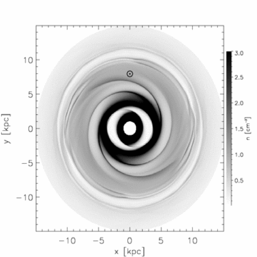
Figure 1.— Density distribution of the simulation after $1\mbox{\,Gyr}$ of evolution. The grayscale shows the gas density in units of $\mbox{\,cm}^{-3}$. It is noticeable that, although the perturbation has only two arms, the gas response shows four arms. The Sun symbol shows the position chosen for the imaginary observer.

Figure 1 shows the simulation after $1\mbox{\,Gyr}$ of evolution. The most important characteristics of the simulation at this stage are: 1) although the perturbation consists of two spiral arms, the gas forms four arms (two pairs with pitch angles of $9^{\mbox{\small o}}$ and $13^{\mbox{\small o}}$ each, as opposed to the perturbation with a pitch angle of $15.5^{\mbox{\small o}}$); 2) a high density ring is formed at $r\approx 4\mbox{\,kpc}$; and, 3) a low density ring is formed near corotation, at $r\approx 11\mbox{\,kpc}$. Again, details of the simulation and the physical phenomena related to these structures are discussed elsewhere. The corotation low density ring was found (using a different background potential) by Martos & Yáñez (private communication). A study of the neccesary conditions for the formation of such ring, its physics and consequences for our Galaxy is presented in Martos (2006, in preparation).

Gómez & Cox (2004a, b) also performed large scale simulations of the Galaxy. Since their numerical model was three-dimensional, they were able to study some phenomena (like the vertical motions associated to the hydraulic jump behavior of the gas near the spiral arms) that could have an impact in the dynamics of the gas near the midplane. Nevertheless, the focus of their model was to study those phenomena, and an emulation of the Milky Way Galaxy was not a priority. Specifically, their three-dimensional numerical grid, a necessity in their work, restricted the spatial resolution achivable in the midplane. This, together with the low value for $\Omega_{P}$ used, did not allow the formation of four spiral arms as a response to a two-arm spiral potential (in order to obtain four gaseous arms, their model included a four-arm potential). In the present work, the model was restricted to the galactic plane so that sufficient resolution can be reached.

Figure 2.— Column density, in arbitrary units, vs. galactic longitude in the simulation. By moving the imaginary observer around a circle of radius $R_{\odot}=8\mbox{\,kpc}$, the local maxima can be matched to the observed directions tangent to the spiral arms (thick vertical lines). The dashed area at $|l|<7^{\mbox{\small o}}$ shows the simulation inner radial boundary.

3. THE SYNTHETIC OBSERVATIONS

Local maxima in column density ($N$) vs. galactic longitude ($l$) plots for the diffuse gas are usually interpreted as the directions at which the line-of-sight is tangent to spiral arms. The $N$ vs. $l$ distribution an imaginary observer would see if placed inside this model galaxy is presented in Figure 2. By moving the observer around the solar circle, at $8\mbox{\,kpc}$ in the numerical model, the number and positions of the local maxima can be fitted to the observed values for the diffuse gas. In this work, the chosen directions were those tangent to the locus of the spiral arms proposed by Taylor & Cordes (1993), namely, $l=-76.5^{\mbox{\small o}},-51.6^{\mbox{\small o}},-32.4^{\mbox{\small o}},32.7^{\mbox{\small o}}$ and $47.1^{\mbox{\small o}}$. It was found that by choosing the position shown in Figure 1 for the imaginary observer all but one of the column density local maxima in the model fall within $3^{\mbox{\small o}}$ of these quoted directions. If the tangent directions quoted by Drimmel & Spergel (2001) are adopted, namely $l\approx-80^{\mbox{\small o}},\pm 50^{\mbox{\small o}}$ and $\pm 30^{\mbox{\small o}}$, all but one of the tangent directions yield an even better fit. (The difference between the ill-fitting tangent in the model, at $l\approx-72^{\mbox{\small o}}$, and the quoted direction is in fact smaller than the width of the feature observed in $240\,\mu\mbox{m}$. See, for example, Drimmel 2000 and Drimmel & Spergel 2001.)

3.1. The rotation curve

Once a position for the observer is chosen, the next step toward calculating the kinematic distances is to adopt a rotation curve for the simulated galaxy. For the inner galaxy ($r<R_{\odot}$), the standard procedure consists in searching for the terminal velocity of the gas, i.e., the maximum line-of-sight component of the velocity (minimum, for negative longitudes). If one assumes that the gas orbits are circular, the terminal velocity arises from the point at which the line-of-sight is tangent to the orbit, and so, the galactocentric radius of the emitting gas is known. Under this assumption, the circular rotation curve for the galaxy is given by:

$$v_{c}(r)=v_{t}(l)+v_{\odot}\sin(l),$$ (3)

where $v_{c}$ is the circular velocity, $v_{t}(l)$ is the terminal velocity for a given galactic longitude, $v_{\odot}$ is the velocity at the solar circle, and $r=R_{\odot}\sin(l)$ is the galactocentric radius of the tangent point.

At this point, a choice between two options for the value of the circular velocity at the solar circle has to be made. One option is to take the circular velocity consistent with the background gravitational potential ($v_{\odot}=220\mbox{\,km s}^{-1}$). This option has the disadvantage that the gas in the evolved simulation will stream by the observer [although this is not necessarily wrong, since the presence of gas at forbidden velocities in the $l-v$ diagram is well known (Linblad, 1967; Blitz & Spergel, 1991)]. Nevertheless, it was decided in this work to take a second option, which is to take the value for $v_{\odot}$ ($=225\mbox{\,km s}^{-1}$) given by the azimuthal velocity of the gas in the evolved simulation at the position assigned to the imaginary observer, since this choice would more closely mimic the procedure used to determine the Local Standard of Rest from galactic sources (Binney & Merrifield, 1998). There will still be streaming gas, but this will happen in the radial direction only. Such radially streaming gas has been reported by Brand & Blitz (1993).

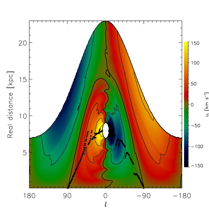
Figure 3.— Line-of-sight component of the velocity field as a function of galactic longitude and (real) distance to the observer, with contours every $50\mbox{\,km s}^{-1}$ (the thicker contour marks the $u_{r}=0\mbox{\,km s}^{-1}$ level). The dotted line shows the locus of the tangent points, while the circles show the positions at which the terminal velocity is reached.

Figure 3 shows the line-of-sight component of the velocity field. The Figure also shows the actual positions at which the terminal velocity is reached for a given $l$. Although the distance between those terminal-velocity points and the tangent points is typically small, the non-circular motions and spiral shocks generate kpc-scale deviations and discontinuities in the terminal-velocity locus. Since those deviations happen at the positions of the spiral arms, they will generate larger errors at the vicinity of the arms, and will strongly affect the observer’s view of the spiral structure of the model galaxy.

For the outer galaxy ($r>R_{\odot}$), the usual procedure to determine the rotation curve involves looking for sources with independently known distance and measuring their line-of-sight velocity (Brand & Blitz, 1993, for example). This procedure was simulated by assuming that the observer finds such a source at each point of the numerical grid outside the solar circle. It is assumed that the distances to such sources are less reliable the farther they are from the observer. So, the circular velocity for the outer galaxy was taken to be,

$$v_{c}(r)=\frac{r}{R_{\odot}}\left(\sum\limits_{\phi}\frac{w_{\phi}v_{los}}{\sin(l)}+v_{\odot}\right),$$ (4)

where the weights $w_{\phi}$ decrease linearly with the distance to the observer, and the summation is performed, at a given radius, over the azimuthal points excluding those within $7^{\mbox{\small o}}$ of the galactic center and anti-center directions.

Figure 4.— a) The rotation curve given by the background potential (solid line), compared with the measured rotation curve. For the inner galaxy, both the rotation measured for positive (dotted line) and negative longitudes (dashed line) are presented. The rotation curve corresponding to the outer galaxy is also shown (dashed-dotted line). b) The rotation curve given by the background potential (solid line), compared with the average of the north and south rotation curves (dotted line) and the mean azimuthal velocity of the gas in the simulation (dashed line). Notice that both the mean velocity and the mean rotation curve are above the background rotation curve for most of the radial domain.

Figure 4(a) shows the so obtained rotation curves, together with the rotation consistent with the background gravitational potential. The northern rotation curve is lower than the southern rotation at $\sim 3.5\mbox{\,kpc}<r<\sim 5.5\mbox{\,kpc}$, while the opposite is true up to $r=R_{\odot}$. This behavior is similar to the rotation curves reported by Blitz & Spergel (1991), when scaled for $R_{\odot}=8\mbox{\,kpc}$.

In order to try to recuperate the true (background) rotation, that should more closely trace the large scale mass distribution, the average both northern and southern rotation curves was taken. The result is compared with the background rotation in Figure 4(b). Although the result is smoother and closer to the rotation consistent with the background potential, it is still systematically higher (in agreement with the results reported by Sinha, 1978). Another approach is to take the full velocity field and average the azimuthal velocity of the gas (Brand & Blitz, 1993). The result, also shown in Figure 4(b), is much closer to the background rotation, but it is still systematically larger.

4. ERRORS IN THE KINEMATIC DISTANCE

After adopting a rotation curve, and assuming that the gas follows circular orbits, the errors in the measured kinematic distances can be estimated by comparing the measured with the real distance in the simulation.

In order to resolve the distance ambiguity for the inner galaxy, the usual procedure is to bracket the distance close enough as to place the object of interest on either side of the tangent point by looking at the galactic lattitude extension of the source (Fish et al., 2003), or using observed intermediate absorption features (Watson et al., 2003; Sewilo et al., 2004). For this investigation, I decided to cheat: I looked up on which side of the tangent point the gas parcel fell on, and chose the measured distance accordingly.

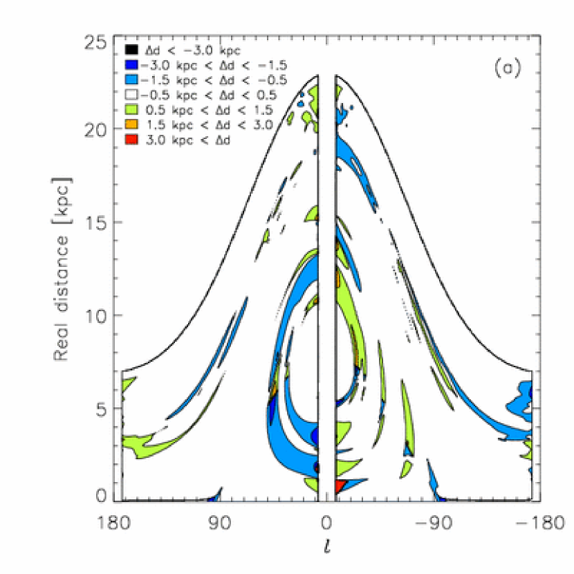
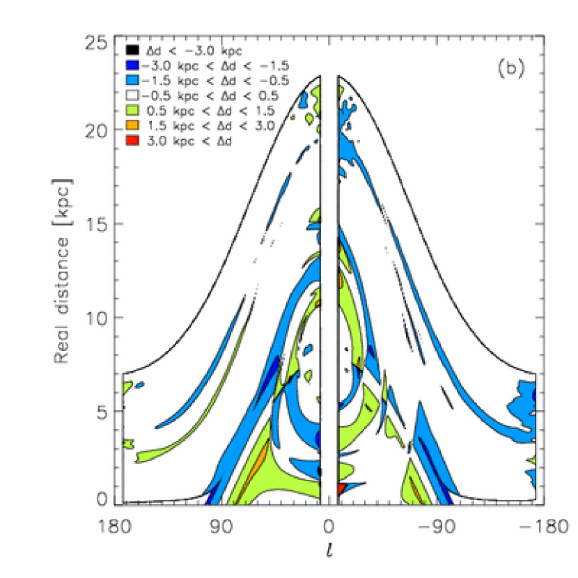
Figure 5.— Error in the measured kinematic distance ($\Delta d$) obtained under the assumption of circular orbits following (a) the measured rotation curve, and (b) the rotation given by the background potential. Sections of $7^{\mbox{\small o}}$ around the galactic longitudes $l=0^{\mbox{\small o}}$ and $180^{\mbox{\small o}}$ were excluded. Although the error in most of the galactic disk is of the order of $0.5\mbox{\,kpc}$, it is significantly larger at the positions of the spiral arms. The sharp edges at the position of the tangent points are a consequence of the fact that the terminal velocities do not happen at those points. The errors in measured kinematic distances are larger when the real (background) rotation curve is used.

Figure 5(a) shows the error in measured distance with respect to the real distance in the model. Recalling Figure 4, the observer would determine different rotation curves for the northern and southern sides of the galactic center. Accordingly, in determining the kinematic distance for Figure 5(a), the rotation curve used was that of the corresponding side of the galactic center. It is noticeable that although the errors are of the order of $0.5\mbox{\,kpc}$ in most of the galactic disk, they are significantly larger at the positions of the spiral arms (as hinted by Gómez & Cox, 2004b). This fact has a special impact in studies of the spiral structure of the Galaxy that rely on kinematic distances, since it distorts the image the observer would generate (see §4.1).

There is another significant feature in Figure 5. Although the terminal velocity does not really arises from the tangent point, the circular orbits assumption assigns gas observed near terminal velocity to that point. This fact generates a feature in the errors that corresponds to the locus of the tangent points. Again, the error is significant at the position of the spiral arms and would generate large errors in the determination of distances to objects that trace the spiral structure.

The assumptions of circular orbits and different rotation curves for positive and negative longitudes are, of course, inconsistent. One solution is to fit a single rotation curve to both sides of the Galaxy. In order to test this method, the average of both rotation curves was taken and the equivalent of Figure 5(a) was calculated. The result was that the magnitude of the error in the kinematic distances was approximately the same, but the area with error $>0.5\mbox{\,kpc}$ spanned a larger fraction of the disk.

Suppose now that the imaginary observer somehow manages to obtain the large scale distribution of stellar mass in the model galaxy. This would allow the derivation of the real rotation curve from the background axisymmetric potential. If the observer now uses that real rotation to determine kinematic distances, even larger distance errors would be obtained, specially for the inner galaxy, as shown in Figure 5(b). This counter-intuitive fact arises because, at this point of the simulation, the gas has already adopted orbits that are not only influenced by the background potential, but also the large scale magnetic field (likely different from the field in the initial conditions) and the torques and resonances generated by the spiral perturbation. Although the real rotation curve is consistent with the most important determinant of the gas rotation velocity (the background mass distribution), it does not include other influences in that velocity, while the “wrong” rotation curve determined from gaseous terminal velocities more closely reflects the real motion of the gas (recall Fig. 4, where the measured rotation curve is systematically above the true rotation).

Although intrinsically inconsistent, the two different measured rotation curves were used in the remaining of this investigation since that procedure leads to smaller distance errors. The results presented in the following section are even more notorious if the average or the real rotation curves are used.

4.1. The Galaxy Distorted.

Consider now that the imaginary observer tries to study the spiral structure of the galaxy he/she lives in. The procedure would consist of translating the longitude-velocity data obtained from a diffuse gas survey, for example, into a spatial distribution using the kinematic distances that result from the assumption of circular orbits that follow the measured rotation curve. The resulting map is shown in Figure 6. Notice that the features described for Figure 1 (namely the four spiral arms, the $4\mbox{\,kpc}$ high density ring, and the corotation low density ring) all but disappear, while new fictitious features, like the structure in the outer Galaxy, are formed as a consequence of the oscillations in the outer rotation curve. Also significant in this Figure are the regions where little or no gas is assigned by the mapping, namely the bands near the corotation circle and the quasi-triangular regions near the tangent point locus. (This nearly empty regions are significantly larger when the background or the mean rotation curves were used to determine the distance to the observed gas parcel.)

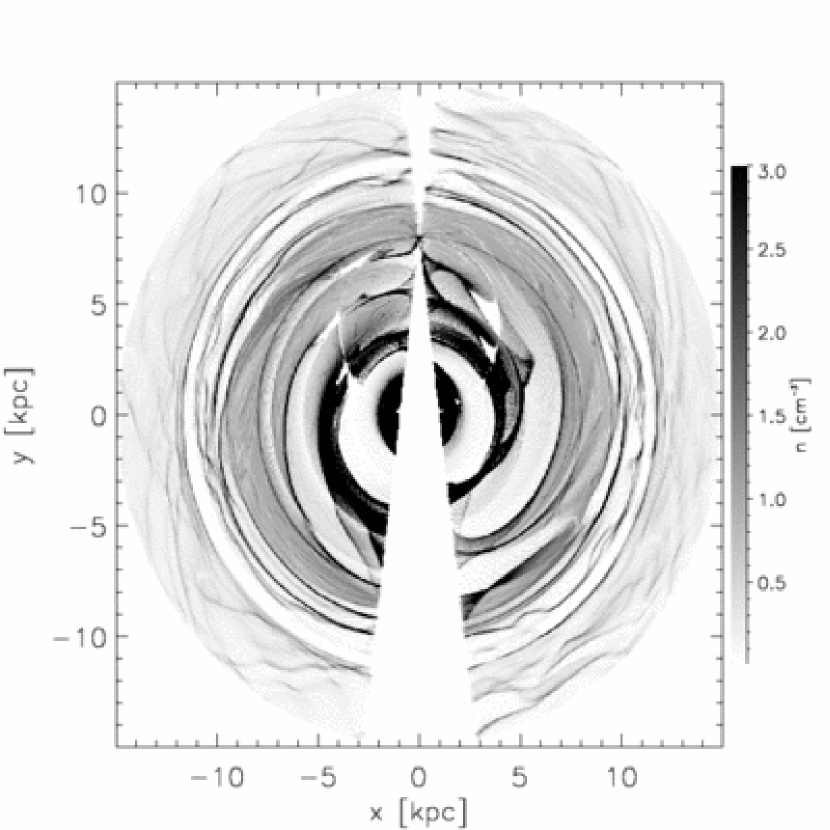
Figure 6.— Re-mapping of the gas distribution resulting from the kinematic distances using the measured rotation curves in Figure 4(a) and assuming circular gas orbits. Notice the regions near the tangent points and the corotation circle, where little or no gas is mapped to.

The imaginary observer would likely conclude that his/her home galaxy has 2 ill-defined spiral arms. If a logarithmic spiral model were forced, an $\sim 11^{\mbox{\small o}}$ pitch angle and a density contrast much stronger than that in the numerical model would be found.

Another possibility for determining the distance to a gas parcel consists in comparing the line-of-sight velocity of the parcel with the predicted velocity obtained from some model for the galactic structure. For the numerical model described in §2, given a galactic longitude, Figure 3 is searched for the required velocity, and the corresponding distance is read out. Although the same procedure to solve the ambiguity with respect to the tangent point was used, the non-circular motions introduce new distance ambiguities for certain longitude-velocity values (up to 11, although 3 is a more typical number). When these ambiguities appear, they happen close to each other, making their resolution difficult. So, when reconstructing the map of the galaxy, the gas density was equally split among these positions.

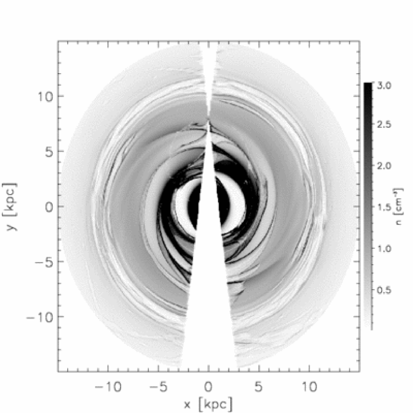
Figure 7.— Same as Figure 6, but using the full velocity field to recover the density distribution. Most of the characteristics of Figure 1 are recovered, although some spurious structure appears due to the new distance ambiguities introduced by the non-circular motions.

The result is shown in Figure 7. The new distance ambiguities still introduce spurious structure, like the splitting of the spiral arms. Nevertheless, the number and position of the arms, the structure around the corotation radius and the lack of features in the outer galaxy are recovered. The imaginary observer would likely conclude that his/her home galaxy has 4 arms with $9^{\mbox{\small o}}$ and $12.5^{\mbox{\small o}}$ pitch angles, although he/she would also find non-existing bridges and spurs. On the other hand, it should be considered that the imaginary observer does not see thermal nor turbulent line broadening. When these are considered, some of the new ambiguities will be swallowed into a distance range, effectively dissapearing. Therefore, some of the spurious structures will blend with real structures. So, the observer might get an image of the model galaxy closer to reality than Figure 7 suggests.

5. SUMMARY AND DISCUSSION

The effect of the circular orbits assumption on our idea of the large scale structure of the Galaxy was explored. Since these errors might be quite large at the position of the spiral arms, the study of the spiral structure of the Galaxy and objects associated with it is particularly affected. By simulating the way an imaginary observer inside the model galaxy might try to infer the structure of the gaseous disk, it was found that the circular orbits assumption destroys the spiral structure and creates spurious features in the measured distribution.

The method of kinematic distances is a powerful one since it allows measurement of distances to diffuse sources and it is easily applicable to a large fraction of the galactic disk. Even if the measured rotation curve includes deviations that do not reflect the true large scale mass distribution, Figure 5(a) shows that the errors in the distance are, in fact not very large for most of the galactic disk; in fact, the distance errors that arise from using the true rotation curve are larger. In both cases, however, the errors are quite large at the positions of the spiral arms. If we want to use this distance method for objects associated with the spiral structure, we need to consider non-circular motions (as has been succesfully shown by Foster & MacWilliams, 2006 for a set of H II regions and SNR).

One possibility to achieve this is to try to determine the full velocity field of the galactic disk. But direct measure of distances to the diffuse gas component is quite difficult (therefore the strength of the kinematic distance method). So, we need to use discreet objects and assume that they share their velocity with the diffuse component (Brand & Blitz, 1993, for example; Minn & Greenberg, 1973, see also discussion in). Yet another difficulty arises when tangential velocities and distances are required beyond the solar neighborhood.

Another approach at determining the full velocity field is to model it. Recently, Foster & MacWilliams (2006) used an analytical model of the density and velocity fields of the diffuse gas, with parameters for the model fitted to H I observations of the outer Galaxy. Despite the fact that their density and velocity models are not consistent in the hydrodynamics sense, and that the model do not include the dynamical effects of magnetic fields, they were able to add features of the Galaxy that are currently difficult to incorporate to numerical models, like the disk’s warp or the rolling motions associated with the spiral arms. Further numerical studies should allow the development of a more realistic analytical model.

Instead of an analytic model, a numerical model was used in the present work to obtain density and velocity fields. Since the focus is in large scale velocity structures, an eulerian code provides a good approach. Also, since the galactic magnetic field has been proved to be an important component of the total ISM pressure (Boulares & Cox, 1990), its effect in the gas dynamics is likely to be important; therefore, a full MHD simulation was required. The large scale forcing is also trascendant; since the azimuthal shape of the spiral perturbation appears to have an influence on the gaseous response (Franco et al., 2002), the usual sinusoidal perturbation was deemed too simplistic and a self-consistent model for the perturbing arms was chosen. At the present time, the galactic warp and the vertical motions associated with the spiral arms (Gómez & Cox, 2004a, b) could not be considered at the necessary resolution.

In this work, it has been shown that it is possible to recover most of the gaseous structure of the galactic disk using kinematic distances, as long as the full velocity field is considered. Nevertheless, applying these results to the Milky Way is a whole new issue, since obtaining the full velocity field is not trivial. For the procedure used here, how close the numerical simulation is to the real Galaxy remains the weak point of this approach. The computation cost of a realistic enough simulation is still too high to allow a parameter fitting analysis. So, the remaining question is if the velocity field that results from the simulation yields a determination of the distance to a given object, or only an estimation of the distance error. The answer to that question is left to the reader’s criterion.

References

- Binney & Merrifield (1998) Binney, J. & Merrifield, M. 1998, Galactic Astronomy (Princeton: Princeton Univ. Press)
- Blitz & Spergel (1991) Blitz, L. & Spergel, D. N. 1991, ApJ, 370, 205
- Boulares & Cox (1990) Boulares, A. & Cox, D. P. 1990, ApJ, 365, 544
- Brand & Blitz (1993) Brand, J. & Blitz, L. 1993, A&A, 275, 67
- Dehnen & Binney (1998) Dehnen, W. & Binney, J. 1998, MNRAS, 294, 429
- Drimmel (2000) Drimmel, R. 2000, A&A, 358, L13
- Drimmel & Spergel (2001) Dimmel, R. & Spergel, D. N. 2001, ApJ, 556, 181
- Fish et al. (2003) Fish, V. L., Reid, M. J., Wilner, D. J. & Churchwell, E. 2003, ApJ, 587, 701
- Foster & MacWilliams (2006) Foster, T. & MacWilliams, J. 2006, ApJ, 644, 214
- Franco et al. (2002) Franco, J., Martos, M., Pichardo, B. & Jongsoo, K. 2002, ASP Conf. Ser. 275, Disks of Galaxies: Kinematics, Dynamics and Perturbations, ed. E. Athanassoula, A. Bosma & R. Mujica (San Francisco: ASP) 343
- Georgelin & Georgelin (1976) Georgelin, Y. M. & Georgelin, Y. P. 1976, A&A, 49, 57
- Gómez & Cox (2004a) Gómez, G. C. & Cox, D. P. 2004a, ApJ, 615, 744
- Gómez & Cox (2004b) — 2004b, ApJ, 615, 758
- Kerr (1962) Kerr, F. J. 1962, MNRAS, 123, 327
- Kerr (1969) — 1969, ARA&A, 7, 39
- Linblad (1967) Linblad, P. O. 1967, Bull. Astron. Inst. Neth., 19, 34
- Maciel & Lago (2005) Maciel, W. J. & Lago, L. G. 2005, RevMexAA, 41, 383
- Martos et al. (2004a) Martos, M., Hernández, X., Yáñez, M., Moreno, E., Pichardo, B. 2004a, MNRAS, 350, L47
- Martos et al. (2004b) Martos, M., Yáñez, M., Hernández, X., Moreno, E., Pichardo, B. 2004b, JKAS, 37, 199
- Minn & Greenberg (1973) Minn, Y. K. & Greenberg, J. M. 1973, A&A, 24, 393
- Oort et al. (1958) Oort, J. H., Kerr, F. J. & Westerhout, G. 1958, MNRAS, 118, 379
- Pichardo et al. (2003) Pichardo, B., Martos, M., Moreno, E. & Espresate, J. 2003, ApJ, 582, 230
- Sewilo et al. (2004) Sewilo, M., Watson, C., Araya, E., Churchwell, E., Hofner, P. & Kurtz, S. 2004, ApJS, 154, 553
- Sinha (1978) Sinha, R. P. 1978, A&A, 69, 227
- Stone & Norman (1992a) Stone, J. M. & Norman, M. L. 1992a, ApJS, 80, 753
- Stone & Norman (1992b) — 1992b, ApJS, 80, 791
- Taylor & Cordes (1993) Taylor, J. H. & Cordes, J. M. 1993, ApJ, 411, 674
- Watson et al. (2003) Watson, C., Araya, E., Sewilo, M., Churchwell, E., Hofner, P. & Kurtz, S. 2003, ApJ, 587, 714
- Yáñez (2005) Yáñez, M. A. 2005 Ph.D. thesis, U.N.A.M.