Structure of Magnetic Tower Jets in Stratified Atmospheres

Abstract

Based on a new approach on modeling the magnetically dominated outflows from AGNs (Li et al. 2006), we study the propagation of magnetic tower jets in gravitationally stratified atmospheres (such as a galaxy cluster environment) in large scales ($>$ tens of kpc) by performing three-dimensional magnetohydrodynamic (MHD) simulations. We present the detailed analysis of the MHD waves, the cylindrical radial force balance, and the collimation of magnetic tower jets. As magnetic energy is injected into a small central volume over a finite amount of time, the magnetic fields expand down the background density gradient, forming a collimated jet and an expanded “lobe” due to the gradually decreasing background density and pressure. Both the jet and lobes are magnetically dominated. In addition, the injection and expansion produce a hydrodynamic shock wave that is moving ahead of and enclosing the magnetic tower jet. This shock can eventually break the hydrostatic equilibrium in the ambient medium and cause a global gravitational contraction. This contraction produces a strong compression at the head of the magnetic tower front and helps to collimate radially to produce a slender-shaped jet. At the outer edge of the jet, the magnetic pressure is balanced by the background (modified) gas pressure, without any significant contribution from the hoop stress. On the other hand, along the central axis of the jet, hoop stress is the dominant force in shaping the central collimation of the poloidal current. The system, which possesses a highly wound helical magnetic configuration, never quite reaches a force-free equilibrium state though the evolution becomes much slower at late stages. The simulations were performed without any initial perturbations so the overall structures of the jet remain mostly axisymmetric.

1. INTRODUCTION

A number of astronomical systems have been discovered to eject tightly collimated and hyper-sonic plasma beams and large amounts of magnetic fields into the interstellar, intracluster and intergalactic medium from the central objects during their initial/final (often violent) stages. Magnetohydrodynamic (MHD) mechanisms are frequently invoked to model the launching, acceleration and collimation of jets from Young Stellar Objects (YSOs), X-ray binaries (XRBs), Active Galactic Nuclei (AGNs), Microquasars, and Quasars (QSOs) (see, e.g., Meier, Koide, & Uchida, 2001, and references therein).

Theory of magnetically driven outflows in the electromagnetic regime has been proposed by Blandford (1976) and Lovelace (1976) and subsequently applied to rotating black holes (Blandford & Znajek, 1977) and to magnetized accretion disks (Blandford & Payne, 1982). By definition, these outflows initially are dominated by electromagnetic forces close to the central engine. In these and subsequent models of magnetically driven outflows (jets/winds), the plasma velocity passes successively through the hydrodynamic (HD) sonic, slow-magnetosonic, Alfvénic, and fast-magnetosonic critical surfaces.

The first attempt to investigate the nonlinear (time-dependent) behavior of magnetically driven outflows from accretion disks was performed by Uchida & Shibata (1985). The differential rotation in the system (central star/black hole and the accretion disk) creates a magnetic coil that simultaneously expels and pinches some of the infalling material. The buildup of the azimuthal (toroidal) field component in the accretion disk is released along the poloidal field lines as large-amplitude torsional Alfvén waves (“sweeping magnetic twist”). After their pioneering work, a number of numerical simulations to study the MHD jets have been done (see, e.g., Ferrari, 1998, and references therein). An underlying large-scale poloidal field for producing the magnetically driven jets is almost universally assumed in many theoretical/numerical models. However, the origin and existence of such a galactic magnetic field are still poorly understood.

In contrast with the large-scale field models, Lynden-Bell (Lynden-Bell & Boily, 1994; Lynden-Bell, 1996, 2003, 2006) examined the expansion of the local force-free magnetic loops anchored to the star and the accretion disk by using the semi-analytic approach. Twisted magnetic fluxes due to the disk rotation make the magnetic loops unstable and splay out at a semi-angle 60° from the rotational axis of the disk. Global magnetostatic solutions of magnetic towers with external thermal pressure were also computed by Li et al. (2001) using the Grad-Shafranov equation in axisymmetry (see also, Lovelace et al., 2002; Lovelace & Romanova, 2003; Uzdensky & MacFadyen, 2006). Full MHD numerical simulations of magnetic towers have been performed in two-dimension (axisymmetric) (Romanova et al., 1998; Turner, Bodenheimer, & Różyczka, 1999; Ustyugova et al., 2000; Kudoh, Matsumoto & Shibata, 2002; Kato, Hayashi, & Matsumoto, 2004) and three-dimension (Kato, Mineshige, & Shibata, 2004). Magnetic towers are also observed in the laboratory experiments (Hsu & Bellan, 2002; Lebedev et al., 2005).

This paper describes the nonlinear dynamics of propagating magnetic tower jets in large scales ($>$ tens of kpc) based on three-dimensional MHD simulations. We follow closely the approach described in Li et al. (2006; hereafter Paper I). Different from Paper I, which studied the dynamics of magnetic field evolution in a uniform background medium, we present results on the injection and the subsequent expansion of magnetic fields in a stably stratified background medium that is described by an iso-thermal King model (King, 1962). Since the simulated magnetic structures traverse several scale heights of the background medium, we regard that our simulations can be compared with the radio sources inside the galaxy cluster core regions. Due to limited numerical dynamic range, however, the injection region (see Paper I) assumed in this paper will be large (a few kpc). Our goal here is to provide the detailed analysis of the magnetic tower jets, in terms of its MHD wave structures, its cylindrical radial force balance, and collimation. The paper is organized as follows: In §2, we outline the model and numerical methods. In §3, we describe the simulation results. Discussions and conclusions are given in §4 and §5.

2. MODEL ASSUMPTIONS AND NUMERICAL METHODS

The basic model assumptions and numerical treatments we adopt here are essentially the same as those in Paper I. Magnetic fluxes and energy are injected into a characteristic central volume over a finite duration. The injected fluxes are not force-free so that Lorentz forces cause them to expand, interacting with the background medium. For the sake of completeness, we show the basic equations and other essential numerical setup here again, and refer readers to Paper I for more details.

2.1. Basic Equations

We solve the nonlinear system of time-dependent ideal MHD equations numerically in a 3-D Cartesian coordinate system ($x,\,y,\,z$):

$$\frac{\partial\rho}{\partial t}+\nabla\cdot(\rho\mbox{\bf V}) = \dot{\rho}_{\rm inj}$$ (1)

$$\frac{\partial(\rho{\bf V})}{\partial t}+\nabla\cdot\left(\rho{\bf VV}+p+B^{2}/2-{\bf BB}\right) = -\rho\nabla\psi$$ (2)

$$\frac{\partial E}{\partial t}+\nabla\cdot\left[\left(E+p+B^{2}/2\right){\bf v}-{\bf B}({\bf v}\cdot{\bf B})\right] = -\rho{\bm{V}}\cdot\nabla\psi$$ (3)

$$+ \dot{E}_{\rm inj}$$

$$\frac{\partial{\bf B}}{\partial t}-\nabla\times({\bf V}\times{\bf B}) = {\dot{\bf B}}_{\rm inj},$$ (4)

Here $\rho$, $p$, ${\bm{V}}$, ${\bm{B}}$, and $E$ denote the mass density, hydrodynamic (gas) pressure, fluid velocity, magnetic field, and total energy, respectively. The total energy $E$ is defined as $E=p/(\gamma-1)+\rho V^{2}/2+B^{2}/2$, where $\gamma$ is the ratio of the specific heats (a value of $5/3$ is used). The Newtonian gravity is $-\nabla\psi$. Quantities $\dot{\rho}_{\rm inj}$, $\dot{{\bm{B}}}_{\rm inj}$, and $\dot{E}_{\rm inj}$ represent the time-dependent injections of mass, magnetic flux, and energy, whose expressions are given in Paper I.

We normalize physical quantities with the unit length scale $R_{0}$, density $\rho_{0}$, velocity $V_{0}$ in the system, and other quantities derived from their combinations, e.g., time as $R_{0}/V_{0}$, etc. These normalizing factors are summarized in Table 1. Hereafter, we will use the normalized variables throughout the paper. Note that a factor of $4\pi$ has been absorbed into the scaling for both the magnetic field ${{\bm{B}}}$ and the corresponding current density ${{\bm{J}}}$. To put our normalized physical quantities in an astrophysical context, we use the parameters derived from the X-ray observations of the Perseus cluster as an example (Churazov et al., 2003). These values are also given in Table 1.

The system of dimensionless equations is integrated in time by using an upwind scheme (Li & Li, 2003). Computations were performed on the parallel Linux clusters at LANL.

2.2. Initial and Boundary Conditions

One key difference from Paper I is that we now introduce a non-uniform background medium. An iso-thermal model (King, 1962) has been adopted to model a gravitationally stratified ambient medium. This is applicable, for example, to modeling the magnetic towers from AGNs in galaxy clusters.

The initial distributions of the background density $\rho$ and gas pressure $p$ are assumed to be

$$\rho=p=\left[1+\left(\frac{R}{R_{\rm c}}\right)^{2}\right]^{-\kappa},$$ (5)

where $R=(x^{2}+y^{2}+z^{2})^{1/2}$ is the spherical radius and $R_{\rm c}$ the cluster core radius. (In the following discussion, both “transverse” and “radial” have the same meaning, referring to the cylindrical radial direction.) The parameter $\kappa$ controls the gradient of the ambient medium. Furthermore, we assume that the ambient gas is initially in a hydrostatic equilibrium under a fixed (in time and space) yet distributed gravitational field $-\nabla\psi(R)$ (such as that generated by a dark matter potential). From the initial equilibrium, we get

$$-\nabla\psi=\frac{\nabla p|_{t=0}}{\rho|_{t=0}}=-\frac{2\kappa R}{R_{\rm c}^{2}}\left[1+\left(\frac{R}{R_{\rm c}^{2}}\right)^{2}\right]^{-1}.$$ (6)

In the present paper, we choose $R_{\rm c}=4.0$ and $\kappa=1.0$. The initial sound speed in the system is constant, $C_{\rm s}|_{t=0}={\gamma}^{1/2}\approx 1.29$, throughout the computational domain. An important time scale is the sound crossing time $\tau(\equiv R/C_{\rm s})\approx 0.78$, normalized with $\tau_{\rm s0}(\equiv R_{0}/C_{\rm s0})\approx 10.0$ Myrs. Therefore, a unit time scale $t=1$ corresponds to $12.8$ Myrs.

The total computational domain is taken to be $|x|\leq 16$, $|y|\leq 16$, and $|z|\leq 16$ corresponding to a $(80\ {\rm kpc})^{3}$ box in the actual length scales. The numbers of grid points in the simulations reported here are $N_{x}\times N_{y}\times N_{z}=240\times 240\times 240$, where the grid points are assigned uniformly in the $x$, $y$, and $z$ directions. A cell $\Delta x\ (=\Delta y=\Delta z\sim 0.13)$ corresponds to $\sim 0.65\ {\rm kpc}$. We use the outflow boundary conditions at all outer boundaries. Note that for most of the simulation duration, the waves and magnetic fields stay within the simulation box, and all magnetic fields are self-sustained by their internal currents.

2.3. Injections of Magnetic Flux, Mass, and Energy

The injections of magnetic flux, mass and its associated energies are the same as those described in Paper I. The ratio between the toroidal to poloidal fluxes of the injected fields is characterized by a parameter $\alpha=15$, which corresponds to $\sim 6$ times more toroidal flux than poloidal flux. The magnetic field injection rate is described by $\gamma_{b}$ and is set to be $\gamma_{b}=3$. The mass is injected at a rate of $\gamma_{\rho}=0.1$ over a central volume with a characteristic radius $r_{\rho}=0.5$. Magnetic fields and mass are continuously injected for $t_{\rm inj}=3.1$, after which the injection is turned off. These parameters correspond to an magnetic energy injection rate of $\sim 10^{43}$ ergs/s, a mass injection rate of $\sim 0.046M_{\odot}$/yr, and an injection time $\sim 40$ Myrs.

In summary, we have set up an initial stratified cluster medium which is in a hydrostatic equilibrium. The magnetic flux and the mass are steadily injected in a central small volume with a radius of 1. Since these magnetic fields are not in a force-free equilibrium, they will evolve, forming a magnetic tower and interacting with the ambient medium.

3. RESULTS

In this section we examine the nonlinear evolution and the properties of magnetic tower jets in the gravitationally stratified atmosphere.

3.1. Overview of Formation and Propagation of a Magnetic Tower Jet

Before considering our numerical results in detail, it is instructive to give a brief overview of the time development of the magnetic tower jet system. We achieve this by presenting the selected physical quantities using two-dimensional $x-z$ slices at $y=0$. The distributions of density at various times $(t=2.5,\,5.0,\,7.5,\,{\rm and}\,10.0)$ are shown in Fig. 1. At the final stage ($t=10.0$), we see the formation of a quasi-axisymmetric (around the jet axis) magnetic tower jet with low density cavities (a factor of $\sim 30$ smaller than the peak density). Inside these cavities, the Alfvén speed is large $V_{\rm A}\gtrsim 5.0$, while plasma $\beta$ is small ($\beta=2p/B^{2}\lesssim 0.1$). However, the temperature $T$ ($\propto C_{\rm s}^{2}$) becomes large $T\gtrsim 2.5$ ($\sim$ twice the initial constant value); that is, the hotter gas is confined in the low-$\beta$ magnetic tower. The jet possesses a slender hourglass-shaped structure with a radially confined “body” for $|z|\leq 3$, which is likely due to the background pressure profile having a core radius $R_{c}=4$. As the magnetic tower moves into an increasingly lower pressure background, the expanded “lobes” are formed. A quasi-spherical hydrodynamic (HD) shock wave front moves ahead of the magnetic tower.

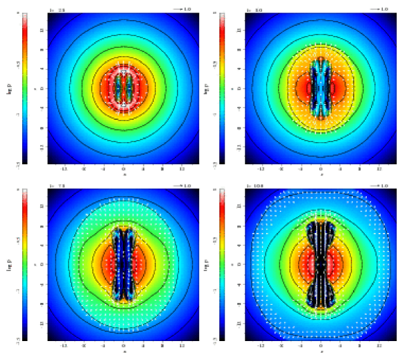
Figure 1.— The density evolution caused by a magnetic tower jet propagating through a stratified background. Color images and contours of the density distribution (logarithmic scale) are shown along with the poloidal velocity field (arrows) in the $x-z$ plane. Density cavities are formed due to the magnetic field expansion. Times are given at the upper left in each of the four panels. The length of the arrow at the upper right in each panel shows the unit velocity.

A snapshot of the gas pressure change ratio $\Delta p/p_{\rm i}=p/p_{\rm i}-1$ (where $p_{\rm i}$ represents $p|_{t=0}$) at $t=10.0$ is shown in Fig. 2. Positive $\Delta p$ can be seen at both the post-shock region of the propagating HD shock wave and just ahead of the magnetic tower ($|z|\sim 8-10$). The distribution of $\Delta p$ forms a “U”-shaped bow-shock-like structure around the head of the magnetic tower. This structure, however, does not appear until $t\sim 7.5$. This is apparently caused by the local compression between the head of the magnetic tower and the reverse MHD slow-mode wave (see discussions in the next section). The gas pressure inside the magnetic tower becomes small ($|\Delta p/p_{\rm i}|\lesssim 0.5$) due to the magnetic flux expansion. Note that the light-blue region between the HD shock and the magnetic tower shows a small pressure decrease ($\Delta p/p_{\rm i}\approx-0.1$). In later sections, we will discuss the origin of this depression and what role it plays in the dynamics of magnetic tower jets.

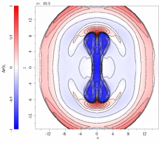
Figure 2.— The change of the gas pressure $\Delta p/p_{\rm i}~{}(\Delta p=p-p_{\rm i})$ ($p_{\rm i}$ represents $p|_{t=0}$) at $t=10.0$ in the $x-z$ plane.

The magnetic tower jet has a well-ordered helical magnetic configuration. The 3-D view of the selected magnetic lines of force, as illustrated in Fig. 3, indicates that a tightly wound central helix goes up along the central axis and a loosely wound helix comes back at the outer edge of the magnetic tower jet. The magnetic pitch $B_{\phi}/\sqrt{B_{r}^{2}+B_{z}^{2}}$ has a broad distribution with a maximum of $\sim 15$. Figure 4 shows a snapshot of the axial current density $J_{z}$ at $t=10.0$. Clearly, the axial current flow displays a closed circulating current system in which it flows along the central axis (the “forward” current ${\bm{J}}^{\rm F}$) and returns on the conically shaped path that is on the outside (the “return” current ${\bm{J}}^{\rm R}$). It is well known that an axial current-carrying cylindrical plasma column with a helical magnetic field is subject to current-driven instabilities, such as sausage ($m=0$), kink ($m=1$), and the other higher order $m$ modes ($m$ is the azimuthal mode number). We however do not see any visible evolution of the non-axisymmetric features in this magnetic tower jet.

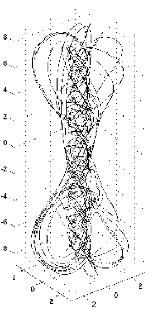
Figure 3.— Three-dimensional configuration view of the selected magnetic lines at $t=10.0$.

From this overview, we see that the magnetic tower jet can propagate through the stratified background medium while keeping well-ordered structures throughout the time evolution. The magnetic fields push away the background gas, forming magnetically dominated, low-density cavities. This action also drives a HD shock wave which is ahead of and eventually separated from the magnetic structures. The magnetic tower has a slender ”body” from the confinement of the background pressure and an expanded “lobe” when the fields expand into a background with the decreasing pressure.

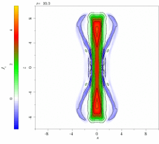
Figure 4.— Distribution of the axial current density $J_{z}$ at $t=10.0$ in the $x-z$ plane. It shows a closed circulating current system, in which the current flows along the central ($z$) column ($J_{z}>0$) and returns along the conically shaped shell on the outside ($J_{z}<0$).

We will now turn to the discussions on the detailed properties of the tower jet, including the HD shock wave and its impact in the axial ($z$) and radial ($x$) directions in §3.2 and 3.3. The radial force balance of the jet is examined in §3.4.

3.2. Structure of a Magnetic Tower Jet in the Axial ($z$) Direction

Figure 5 displays several physical quantities along a line with $(x,y)=(1,0)$ in the axial direction at $t=0.75$. Several features can be identified. First, the HD shock wave front can be seen around $z\sim 13.5$ in the profiles of $\rho$ (top panel), $V_{z}$, and $C_{\rm s}$ (bottom panel). $C_{\rm s}$ is higher than the initial background value $1.29$ in the post-shock region due to shock heating and becomes smaller than $1.29$ at $z\sim 10.7$ due to axial expansion. $V_{z}$ has the similar behavior as $C_{\rm s}$.

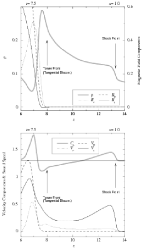
Figure 5.— Axial profiles of physical quantities, parallel to the $z$-axis with $(x,\,y)=(1,\,0)$ at $t=7.5$. Top: Density $\rho$ and magnetic field components $(B_{r},\,B_{\phi},\,B_{z})$. Bottom: Sound speed $C_{\rm s}$ and velocity components $(V_{r},\,V_{\phi},\,V_{z})$. The positions of the expanding hydrodynamic shock wave front and the magnetic tower front, which is identified as a tangential discontinuity, are shown in both panels. A horizontal solid line in the bottom panel denotes the initial sound speed (constant throughout the computational domain).

Second, a magnetic tower front (“tower front” in the following discussions) is located at $z\sim 8.0$, beyond which the magnetic field goes to zero, as seen in the top panel. This indicates that the gas within the magnetic tower jet is separated from the non-magnetized ambient gas beyond the tower front. We regard this front as a tangential discontinuity as the magnetic fields are tangential to the front without the normal component. This is consistent with the fact that the radial and azimuthal field components ($B_{r}$ and $B_{\phi}$) are dominant near the tower front ($z\lesssim 8.0$) but the axial field component $B_{z}$ becomes dominant only for $z<6.0$. The density and pressure show smooth transition through this front though the gradients of $\rho$ and $C_{\rm s}$ are slightly changed there.

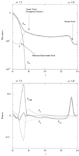
Figure 6.— Similar to Fig. 5. Top: Shown are the gas pressure $p$ (dashed line), magnetic pressure (solid line) $p_{\rm m}$, and total pressure $p_{\rm tot}\,(=p+p_{\rm m})$ (light gray thick solid line). Bottom: Shown are the forces in the axial ($z$) direction: the Lorentz force $F_{{\bm{J}}\times{\bm{B}}}=-\partial/\partial z\left[(B_{r}^{2}+B_{\phi}^{2})/2\right]$, (solid line), gas pressure gradient force $F_{p}=-\partial p/\partial z$ (dashed line), gravitational force $F_{\rm g}=-\rho\partial\psi/\partial R\times|z|/R$ (dotted line), and total force $F_{\rm tot}\,(=F_{{\bm{J}}\times{\bm{B}}}+F_{p}+F_{\rm g})$ (light gray thick solid line). The position of the reverse slow-mode MHD wave front is also shown in the top panel.

Third, there is another MHD wave front at $z\sim 7.0$ where $B_{r}$, $C_{\rm s}$, and every velocity component have their local maxima ($\rho$ instead has its local minimum), as seen in both panels. To better understand the nature of this MHD wave front, we plot the axial profiles of pressures and various forces along the line $(x,y)=(1,0)$ at $t=7.5$ in Fig. 6. The total pressure $p_{\rm tot}$ consists of only the gas pressure $p$ beyond the tower front ($z\gtrsim 8.0$) but is dominated by the magnetic pressure $p_{\rm m}$ behind the MHD wave front ($z\lesssim 7.0$), as seen in the top panel. A transition occurs around $7.0\lesssim z\lesssim 8.0$, where an increase in $p$ is accompanied by a decrease in $p_{\rm m}$. We therefore identify this as a reverse slow-mode compressional MHD wave front. In magnetic towers, the transition region between gas and magnetic pressures can be identified as a reverse slow wave front in the context of MHD wave structures. It does not depend on the resolution and parameters. So, the reverse slow mode wave (sometimes, it can be steepen into a shock) will always be there. In addition, in Fig. 7, we show several snapshots of $V_{z}$ and $p$ during $t=7.5\sim 10.0$ (along the same offset axial path with Figs. 5 and 6). The axial flow is decelerated by the gravitational force in the post-shock region beyond the tower front as seen in the top panel. On the other hand, the narrow region between the tower front and the reverse slow-mode wave front is accelerated by the magnetic pressure gradient (the “magnetic piston” effect). Note that the reverse slow-mode MHD compressional wave could eventually steepen into the reverse slow-mode MHD shock wave via this nonlinear evolution. Consequently, in the frame co-moving with the reverse slow-mode shock, a strong compression occurs behind the shock wave front and causes a local heating, as seen in the bottom panel and also Fig. 2. This heating could have interesting implications for the enhancement of radiation from radio to X-rays at the terminal part of Fanaroff-Riley type II AGN jets, such as lobes and hot spots, which are generally interpreted as heating caused by the jet terminal shock wave (Blandford & Rees, 1974; Scheuer, 1974).

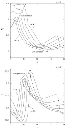
Figure 7.— Similar to Fig. 5, but with selected snapshots during $t=7.5\sim 10.0$ (each time-interval is equal to 0.5). Top: The axial velocity $V_{z}$. Bottom: The gas pressure $p$.

Fourth, the HD shock wave breaks the initial background hydrostatic equilibrium. The passage of the shock wave heats the gas and alters its pressure gradient. As shown in the bottom panel of Fig. 6, the gas pressure gradient force $F_{\rm p}$ stays uupositive at the shock front (which pushes the shock forward), but the total (gravity plus pressure gradient) force $F_{\rm tot}$ becomes negative behind the shock, implying a deceleration of the gas in the axial direction in the post-shock region. This is consistent with Fig. 7.

3.3. Deformation of the Jet “Body” in the Radial Direction

We next examine the structure and dynamics of the magnetic tower jet along the radial direction in the equatorial plane with $(y,z)=(0,0)$. Figure 8 shows the radial profiles of physical quantities along the $x$-axis at $t=6.0$. The boundary of the magnetic tower jet (“tower edge” in the following discussions) is located at $x\sim 3.0$ where $F_{{\bm{J}}\times{\bm{B}}}$ becomes zero. Two distinct peaks of $C_{\rm s}$ and $V_{x}$ around $x\sim$ 7.8 and 9.5 are visible in the top panel. The first front ($x\sim 9.5$) is the propagating HD shock wave front as we showed in the previous section. The second front ($x\sim 7.8$) also indicates another expanding HD shock wave front generated by a bounce when the magnetic flux pinches in the radial direction caused by the “hoop stress”. This secondary shock front appears only in the radial direction (see also Fig. 5). $C_{\rm s}$ decreases gradually towards the jet axis in the post-shock region of the secondary shock and becomes smaller than its initial value $1.29$ at $x\sim 5.7$. We can confirm that these shock fronts are purely powered by the gas pressure gradients $F_{p}$, as seen in the bottom panel (twin peaks of $F_{\rm p}$ are shifted a bit behind that of $C_{\rm s}$ in the top panel).

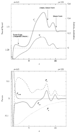
Figure 8.— Radial profiles of physical quantities along the $x$-axis in the equatorial plane with $(y,\,z)=(0,\,0)$ at $t=6.0$. Top: The sound speed $C_{\rm s}$ (light gray thick solid line) and the radial velocity $V_{x}$ (solid line). Bottom: The forces in the radial ($x$) direction: the Lorentz force $F_{{\bm{J}}\times{\bm{B}}}=-\partial/\partial r\left[(B_{\phi}^{2}+B_{z}^{2})/2\right]-B_{\phi}^{2}/r$ (solid line), gas pressure gradient force $F_{p}=-\partial p/\partial r$ (dashed line), gravitational force $F_{\rm g}=-\rho\partial\psi/\partial R\times|x|/R$ (dotted line), and total force $F_{\rm tot}\,(=F_{{\bm{J}}\times{\bm{B}}}+F_{p}+F_{\rm g})$ (light gray thick solid line). The positions of two expanding hydrodynamic shock wave fronts and the edge of the magnetic tower (tangential discontinuity) are shown in the top panel. A horizontal solid line in the top panel denotes the initial sound speed (constant throughout the computational domain) and a horizontal dashed line in the top panel represents a level “0” for the transverse velocity.

Part of the region between the secondary HD shock front and the tower edge has $F_{\rm tot}$ being negative (the bottom panel), meaning that the gas is undergoing gravitational contraction. This is indicated by $V_{x}<0$ in the top panel for $x<5.1$. This behavior is similar to what we have discussed earlier, i.e., the HD shock waves break the background hydrostatic equilibrium, causing a global contraction. Note that this contraction is occurring along the whole jet “body”, e.g., for $|z|\lesssim 4.0$ when $t=7.5$.

The bottom panel also helps to address the question on what forces are confining the magnetic fields in the equatorial plane. Since the total magnetic field $F_{{\bm{J}}\times{\bm{B}}}$ stays positive, this means that the inward hoop stress is not strong enough to confine the magnetic fields. Instead, at the tower edge, it is the background gravity that counters the combined effects of magnetic field pressure and a positive pressure gradient (pushing outward). A bit further into the tower edge (at $x\sim 2.1$), however, the pressure force changes from outwardly directed to inwardly directed. Then, both the pressure gradient and the gravitational forces act to counter the outward ${{\bm{J}}\times{\bm{B}}}$ force. This behavior, which is mostly caused by the magnetic tower expanding in a background gravitational field, is different from the usual MHD models for jets where the inwardly directed hoop stress is balanced by the outwardly directed magnetic pressure gradient (Blandford & Payne, 1982).

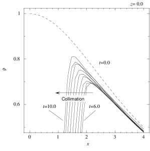
Figure 9.— The radial profiles of density $\rho$ in the equatorial plane with selected snapshots during $t=6.0\sim 10.0$ (each time-interval is equal to 0.5). The initial profile ($t=0.0$) is also shown (dashed line).

To investigate the radius evolution of the magnetic tower jet, we show the radial profile of density at the equatorial plane from $t=6.0$ to $10.0$ in Fig. 9. It shows that the radius has an approximately constant contraction speed for $t=6.5\sim 9.5$. The time scale for contraction is $\tau_{\rm contr}\sim 6$, which is about 7.5 times longer than the local sound-crossing time scale.

3.4. Force Balance in the Radial Direction

We now discuss the jet properties along the radial direction away from the equatorial plane. Figure 10 shows the radial profiles of physical quantities along the $x$-axis with $(y,z)=(0,4)$ at $t=7.5$. The tower edge is now located at $x\sim 3.0$. The plasma $\beta$ in the core of the tower is $\beta\lesssim 0.1$. The top panel shows that the central total pressure (which is dominated by the magnetic pressure) is much bigger than the background “confining” pressure. This illustrates the original suggestion by Lynden-Bell (Lynden-Bell, 1996, 2003) that the hoop stress of the toroidal field component $B_{\phi}$ can act as a pressure amplifier in the central region of the magnetic tower: the pinch effect amplifies $p_{m}$ near the axis of the tower. At the tower edge, however, a finite (albeit small) gas pressure is required (see also Li et al., 2001).

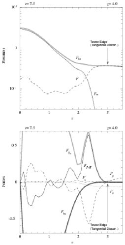
Figure 10.— The radial profiles of physical quantities along the $x$-axis with $(y,\,z)=(0,\,4)$ at $t=7.5$. Top: Similar to the top panel in Fig. 6. Bottom: Similar to the bottom panel in Fig. 8, but with the centrifugal force $F_{\rm c}=\rho V_{\phi}^{2}/r$ (dash-dotted line) and the Lorentz force $F_{{\bm{J}}\times{\bm{B}}}$, which can be separated into the magnetic pressure gradient force $-\partial/\partial r\left[(B_{\phi}^{2}+B_{z}^{2})/2\right]$ (light gray thick solid line) and the hoop stress (magnetic tension force) $-B_{\phi}^{2}/r$ (dark gray thick solid line). The position of the magnetic tower edge (tangential discontinuity) is shown in both panels.

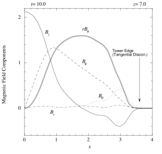
Figure 11.— The radial profiles of the magnetic field components $(B_{r},\,B_{\phi},\,B_{z})$, the poloidal magnetic field $B_{\rm p}=\sqrt{B_{r}^{2}+B_{z}^{2}}$, and the quantity $rB_{\phi}$ along the $x$-axis with $(y,\,z)=(0,\,7)$ at $t=10.0$. The position of the magnetic tower edge (tangential discontinuity) is shown.

The bottom panel shows the detailed distributions of forces along the radial direction. They show that:

• (Region: $x\gtrsim 3.0$) Beyond the tower edge, the gravitational force $F_{\rm g}$ is slightly stronger than the outwardly directed gas pressure gradient force $F_{p}$, indicating that this edge is subject to the gravitational contraction, as discussed in the previous section.

• (Region: $2.0\lesssim x\lesssim 3.0$) Interior to the tower edge, the Lorentz force $F_{{\bm{J}}\times{\bm{B}}}$ is dominated by the outwardly directed magnetic pressure gradient force $F_{p_{m}}$, and it is also larger than the inwardly directed $F_{p}$, indicating that the outer shell of the magnetic shell should be expanding at the relatively higher $z$, in contrast to the equatorial region ($z=0$) where the tower radius is contracting. The hoop stress $F_{\rm hp}$ plays a minor role in the force balance around this region. Note that ${\bm{J}}^{\rm R}$ flows inside this region.

• (Region: $x\lesssim 2.0$) Inside the jet “body”, Contributions from both $F_{p_{m}}$ and $F_{\rm hp}$ become comparable and nearly cancel each other. The residual $F_{{\bm{J}}\times{\bm{B}}}$ is balanced by $F_{p}$ everywhere in this region. $F_{\rm hp}$ becomes dominant in the Lorentz force at the core part. Note that ${\bm{J}}^{\rm F}$ flows within $x\lesssim 1.0$.

In addition, both the $F_{\rm g}$ and the centrifugal force $F_{\rm c}$ play a minor role in terms of the force balance inside the magnetic tower jet. Thus, the interior of the magnetic tower is magnetically dominated but not exactly force-free, i.e., $-\nabla p+{\bm{J}}\times{\bm{B}}\simeq 0~{}~{}$. This small but finite pressure gradient force could potentially provide some stabilizing effects on the traditionally kink-unstable twisted magnetic configurations. The detailed examinations of stability properties in magnetic tower jets will be discussed in a forthcoming paper.

4. DISCUSSIONS

On scales of $\sim$ tens of kpc to hundreds of kpc, the background density and pressure profiles have a strong influence on the overall morphology of the magnetic tower jet. Most notably, the transverse size of the magnetic tower grows as the jet propagates into a decreasing pressure environment, showing a similar morphology with the jet/lobe configuration of radio galaxies.

The radial size of the lobe $r_{\rm lobe}$ can be estimated from the following consideration: Figure 11 shows the radial profiles of magnetic field components parallel to the $x$-axis with $z=7.0$ at $t=10.0$. Together with Fig. 4, we see that both the poloidal field and especially the poloidal current $I_{z}$ maintain well collimated around the central axis even at the late stage of the evolution. This implies that the toroidal magnetic fields in the lobe region are distributed roughly as $B_{\phi}\sim I_{z}/r$. This is consistent with the results shown in Fig. 11 where $rB_{\phi}$ have a plateau from $x\approx 1-2.5$. As indicated in Fig. 10, we see that the magnetic pressure and the background pressure try to balance each other at the tower edge. Thus, we expect that

$$\frac{B_{\rm P}^{2}+B_{\phi}^{2}}{8\pi}\sim p_{\rm e}~{},$$ (7)

where $p_{\rm e}$ is the external gas pressure at the tower edge. When the lobe experiences sufficient expansion, we expect the poloidal field strength to drop much faster than $1/r_{\rm lobe}$. So we have

$$\frac{B_{\phi}^{2}}{8\pi}\sim\frac{(I_{z}/r_{\rm lobe})^{2}}{8\pi}\sim p_{\rm e}~{},$$ (8)

which gives

$$r_{\rm lobe}\sim I_{z}~{}p_{e}^{-1/2}~{}~{}.$$ (9)

This is generally consistent with our numerical result shown in Fig. 1 though it is difficult to make a firm quantitative determination since the lobes have not expanded sufficiently.

To make direct comparison between our simulations and observations, further analysis is clearly needed. Note that for the magnetic tower model, the Alfvén surface is located at the outer edge of the magnetic tower and flow within the magnetic tower is always sub-Alfvénic. This is quite different from the hydromagnetic models where the MHD flow is accelerated and has passed through several critical velocity surfaces, including the Alfvén surface.

5. CONCLUSION

By performing 3-D MHD simulations we have investigated in detail the nonlinear dynamics of magnetic tower jets, which propagate through the stably stratified background that is initially in hydrostatic equilibrium. Our simulations, based on the approach developed in Li et al. (2006), confirm a number of the global characteristics developed in Lynden-Bell (1996, 2003) and Li et al. (2001). The results presented here give additional details for a dynamically evolving jet in a stratified background. The magnetic tower is made of helical magnetic fields, with poloidal flux and poloidal current concentrated around the central axis. The “returning” portion of the poloidal flux and current is distributed on the outer shell of the magnetic tower. Together they form a self-contained system with magnetic fields and associated currents, being confined by the ambient pressure and gravity. The overall morphology exhibits a confined magnetic jet “body” with an expanded “lobe”. The confinement of the “body” comes jointly from the external pressure and the gravity. The formation of the lobe is due to the expansion of magnetic fields in a decreasing background pressure.

A hydrodynamic shock wave initiated by the injection of magnetic energy/flux propagates ahead of the magnetic tower and can break the hydrostatic equilibrium of the ambient medium, causing a global gravitational contraction. As a result, a strong compression occurs in the axial direction between the magnetic tower front and the reverse slow-mode MHD shock wave front that follows. Furthermore, the magnetic tower jets are deformed radially into a slender-shaped body due to the inward-directed flow of the ambient (non-magnetized) gas.

The lobe is magnetically dominated and is likely filled with the toroidal magnetic fields generated by the central poloidal current. At the edge of the magnetic tower jet, the outward-directed magnetic pressure gradient force is balanced by the inward-directed gas pressure gradient force, so the radial width of the magnetic tower can be determined jointly by the magnitude of the poloidal current and the magnitude of the external gas pressure. The highly wound helical magnetic field in the magnetic tower never reaches the force-free equilibrium precisely, but obtains radial force-balance, including the gas pressure gradient inside the magnetic tower.

The stability of the magnetic tower jets will be considered in our forthcoming papers.

Table 1Units of Physical Quantities for Normalization.

Physical Quantities	Description	Normalization Units	Typical Values
$R\,(=\sqrt{x^{2}+y^{2}+z^{2}})$	Length	$R_{0}$	5 Kpc
${{\bm{V}}}$	Velocity field	$C_{\rm s0}$	$4.6\times 10^{7}$ cm/s
$t$	Time	$R_{\rm 0}/C_{\rm s0}$	$1.0\times 10^{7}$ yrs
$\rho$	Density	$\rho_{0}$	$5.0\times 10^{-27}$ g/cm3
$p$	Pressure	$\rho_{0}C_{\rm s0}^{2}$	$1.4\times 10^{-11}$ dyn/cm2
${{\bm{B}}}$	Magnetic field	$\sqrt{4\pi\rho_{0}C^{2}_{\rm s0}}$	17.1 $\mu$G

Note. — The initial value of the density $\rho_{0}$ and sound speed $C_{\rm s0}$ at the origin $(x,\,y,\,z)=(0,\,0,\,0)$ are chosen to be the typical density and velocity in the system. The initial dimensionless density $\rho^{\prime}$ and pressure $p^{\prime}$ at the origin are set to unity. We therefore have the initial dimensionless sound speed $C_{\rm s}^{\prime}=\gamma^{1/2}\approx 1.29$. A characteristic time scale, the initial sound crossing time $\tau_{\rm s0}=R_{0}/C_{\rm s0}=10.0$ Myrs, which corresponds to the dimensionless time scale $\tau\approx 0.78$.

References

- Blandford & Rees (1974) Blandford, R. D., & Rees, M. J. 1974, MNRAS, 169, 395
- Blandford (1976) Blandford, R. D. 1976, MNRAS, 199, 883
- Blandford & Znajek (1977) Blandford, R. D., & Znajek, R. L. 1977, MNRAS, 179, 433
- Blandford & Payne (1982) Blandford, R. D., & Payne, D. G. 1982, MNRAS, 199, 883
- Churazov et al. (2003) Churazov, E., Forman, W., Jones, C., & Böhringer, H. 2003, ApJ, 590, 225
- Ferrari (1998) Ferrari, A. 1998, ARA&A, 36, 539
- Hsu & Bellan (2002) Hsu, S. C., & Bellan, P. M. 2002, MNRAS, 334, 257
- Kato, Hayashi, & Matsumoto (2004) Kato, Y., Hayashi, M. R., & Matsumoto, R. 2004, ApJ, 600, 338
- Kato, Mineshige, & Shibata (2004) Kato, Y., Mineshige, S., & Shibata, K. 2004, ApJ, 605, 307
- King (1962) King, I. 1962, AJ, 67, 471
- Kudoh, Matsumoto & Shibata (2002) Kudoh, T., Matsumoto, R., & Shibata, K. 2002, PASJ, 54, 26
- Lebedev et al. (2005) Lebedev, S. V. et al. 2005, MNRAS, 361, 97
- Li et al. (2001) Li, H., Lovelace, R. V. E., Finn, J. M., & Colgate, S. A. 2001, ApJ, 561, 915
- Li et al. (2006) Li, H., Lapenta, G., Finn, J. M., Li, S., & Colgate, S. A. 2006, ApJ in press (astro-ph/0604469)
- Li & Li (2003) Li, S., & Li, H. 2003, Technical Report, LA-UR-03-8935, Los Alamos National Laboratory
- Lovelace (1976) Lovelace, R. V. E. 1976, Nature, 262, 649
- Lovelace et al. (2002) Lovelace, R. V. E., Li, H., Koldoba, A. V., Ustyugova, G. V., & Romanova, M. M. 2002, ApJ, 572, 445
- Lovelace & Romanova (2003) Lovelace, R. V. E., & Romanova, M. M. 2003, ApJ, 596, L159
- Lynden-Bell (1996) Lynden-Bell, D. 1996, MNRAS, 279, 389
- Lynden-Bell (2003) Lynden-Bell, D. 2003, MNRAS, 341, 1360
- Lynden-Bell (2006) Lynden-Bell, D. 2006, MNRAS in press (astro-ph/0604424)
- Lynden-Bell & Boily (1994) Lynden-Bell, D., & Boily, C. 1994, MNRAS, 267, 146
- Meier, Koide, & Uchida (2001) Meier, D. L., Koide, S., & Uchida, Y. 2001, Science, 291, 84
- Romanova et al. (1998) Romanova, M. M., Ustyugova, G. V., Koldoba, A. V., Chechetkin, V. M., & Lovelace, R. V. E. 1998, ApJ, 500, 703
- Scheuer (1974) Scheuer, P. A. G. 1974, MNRAS, 166, 513
- Turner, Bodenheimer, & Różyczka (1999) Turner, N. J., Bodenheimer, P., & Różyczka M. 1999, ApJ, 524, 12
- Uchida & Shibata (1985) Uchida, Y., & Shibata, K. 1985, PASJ, 37, 515
- Ustyugova et al. (2000) Ustyugova, G. V., Lovelace, R. V. E., Romanova, M. M., Li, H., Colgate, S. A. (2000), ApJ, 541, L21
- Uzdensky & MacFadyen (2006) Uzdensky, D. A., & MacFadyen, A. I. 2006, preprint (astro-ph/0602419)