INTEGRAL observations of the cosmic X-ray background in the 5-100 keV range via occultation by the Earth

Abstract

Aims. We study the spectrum of the cosmic X-ray background (CXB) in energy range $\sim$5-100 keV.

Methods. Early in 2006 the INTEGRAL observatory performed a series of four 30ksec observations with the Earth disk crossing the field of view of the instruments. The modulation of the aperture flux due to occultation of extragalactic objects by the Earth disk was used to obtain the spectrum of the Cosmic X-ray Background(CXB). Various sources of contamination were evaluated, including compact sources, Galactic Ridge emission, CXB reflection by the Earth atmosphere, cosmic ray induced emission by the Earth atmosphere and the Earth auroral emission.

Results. The spectrum of the cosmic X-ray background in the energy band 5-100 keV is obtained. The shape of the spectrum is consistent with that obtained previously by the HEAO-1 observatory, while the normalization is $\sim$10% higher. This difference in normalization can (at least partly) be traced to the different assumptions on the absolute flux from the Crab Nebulae. The increase relative to the earlier adopted value of the absolute flux of the CXB near the energy of maximum luminosity (20-50 keV) has direct implications for the energy release of supermassive black holes in the Universe and their growth at the epoch of the CXB origin.

1 Introduction

It is well established (e.g. Giacconi et al. 2001) that the bulk of the CXB emission below $\sim$5 keV is provided by the numerous active galactic nuclei (AGN) - accreting supermassive black holes, which span large range of redshifts from 0 up to 6. At these low energies X-ray mirror telescopes can directly resolve and count discrete sources. The resolved fraction drops from $\approx$80% at 2-6 keV to 50-70% at 6-10 keV (see Brandt & Hasinger, 2005 for review).

At energies above 10 keV the efficiency of X-ray mirrors declines and at present it is impossible to resolve more than few percent of the CXB emission in this regime. It is believed that AGN still dominate CXB at higher energies (at least up to hundreds of keV), although the extrapolation of the low energy data is complicated by the presence of several distinct populations of AGN with different spectra and intrinsic absorption column densities (Sy I, Sy II and quasars, blazars, etc., see e.g. Setti & Woltjer 1989; Comastri et al. 1995; Zdziarski 1996). At the same time the peak of the CXB luminosity is around 30 keV and accurate measurements of the CXB flux at high energies (even if we can not resolve individual objects) are important to understand the energy release in the Universe and the contribution of various types of objects to it.

Such measurements are complicated because instruments working in the energy range from tens to hundreds keV are often dominated by the internal detector background, caused by the interactions of charged particles with the detector material. To decompose the total background into particle-induced background and the CXB contribution one needs either a very good model of the internal detector background or two observations having different relative contributions of these two components. The latter approach was behind the INTEGRAL observations of the Earth which uses the Earth disk as a natural screen to modulate the CXB flux coming on to the detectors.

A similar approach has already been used for the same purpose in the analysis of early space X-ray experiments. In particular the HEAO-1 observatory used a movable 5 cm thick CsI crystal to partly block the instrument field of view and to modulate the CXB signal (Kinzer et al. 1997, Gruber et al. 1999). Here we report the results of the first INTEGRAL observations of the Earth performed in 2006. During these observations the Earth was drifting through the field of view of the INTEGRAL instruments producing a modulation of the flux with an amplitude of the order of 200 mCrab at 30 keV.

The structure of the paper is as follows. In Section 2 we present the details of the Earth observations with INTEGRAL in 2006. In Section 3 we introduce various components contributing to the light curves recorded by the different instruments. In Section 4 we describe the CXB spectrum derived from the INTEGRAL data. The last section summarizes our findings.

2 Observations

INTEGRAL (The International Gamma-Ray Astrophysics Laboratory; Winkler et al. 2003) is an ESA scientific mission dedicated to fine spectroscopy and imaging of celestial $\gamma$-ray sources in the energy range 15 keV to 10 MeV.

The primary imaging instrument onboard INTEGRAL is IBIS (Ubertini et al. 2003) – a coded-mask aperture telescope with the CdTe-based detector ISGRI (Lebrun et al. 2003). It has a high sensitivity in the $20-200$ keV range and has a spatial resolution of better than 10^′.

The best energy resolution (from $\sim$1.5 to 2.2 keV for energies in the 50-1000 keV range) is provided by the SPI telescope - a coded mask germanium spectrometer consisting of 19 individual Ge detectors(Vedrenne et al., 2003, Attie et al., 2003).

In addition INTEGRAL provides simultaneous monitoring of sources in the X-ray (3–35 keV; JEM-X, see Lund et al. 2003) and optical (V-band, 550 nm; OMC, see Mas-Hesse et al., 2003) energy ranges.

The observations used in the analysis were made in January-February 2006 in four separate periods (Table 1). Each observation lasted about 30 ksec.

Table 1: The list of Earth observations by INTEGRAL. The pointing direction corresponds to the beginning of the observation and is drifting slowly (by $\sim$10’ during each observation). Each observation lasted about 30 ksec.

Revolution	Start Date (UT)	Pointing
		$\alpha,\delta$, deg, J2000
401	2006-01-24	252.0  -60.8
404	2006-02-02	251.4  -61.3
405	2006-02-05	251.1  -61.1
406	2006-02-08	250.9  -60.9

2.1 Observing strategy

The standard observing mode of INTEGRAL requires the Earth limb to be at least 15^∘away from the main axis. This separation is required for the observatory star tracker to operate in a normal way and provide information needed for 3-axis stabilization of the spacecraft. These 15 degrees approximately correspond to the radius of the SPI and IBIS field of views (at zero sensitivity). In particular, SPI has a hexagonal field of view (see Fig.1) with a side to side angular size at zero sensitivity of 30.5^∘. The IBIS field of view is a rectangle having 29^∘on side at zero sensitivity. JEM-X has the smallest field of view with a 13.2^∘diameter at zero response. A special operational procedure was developed by the INTEGRAL Science Operations Centre (ISOC) and the INTEGRAL Mission Operations Centre (MOC), in consultation with the instruments teams, in order to on one hand allow the Earth to be within the FoVs of the instruments and on the other hand to ensure a safe mode of operations. The aim was to maximize the solid angle within the FoVs subtended by the Earth and to have sufficiently long observations.

All observations were performed during the rising part of the 3 days satellite orbit, a few hours after the perigee passage. The Earth center (as seen from the satellite) is making a certain track on the celestial sphere. As a first step (with the star tracker on) the main axis of the satellite was pointed towards the position where the Earth would be $\sim$6 hours after perigee exit. The satellite was then in a controlled 3-axis stabilization while the Earth was drifting towards this point. When the Earth limb came within 15^∘from the main axis the star tracker was switched off. Once the Earth crossed the INTEGRAL FoV and the distance between the satellite axis and the Earth limb became larger than 15^∘   the star tracker was switched back-on restoring the controlled 3-axis stabilization. During the period when the star tracker was off the satellite was passively drifting. The total amplitude of the drift was about 10’ and interpolation of the satellite attitude information before and after the drift allows reconstruction of the satellite orientation at any moment with an accuracy better than 10”. The distance from the Earth during this period varied from $\sim$40,000 to $\sim$100,000 km. When the Earth center was close to the main axis of the satellite the angular size of the Earth (radius) was $\sim$5.4^∘, corresponding to a subtended solid angle of $\sim$90 sq.deg. As is further discussed in section 3 (see also Fig.6 and 7) the modulation of the CXB flux by the Earth disk is the main source of the flux variations observed by JEM-X, IBIS and SPI.

Schematically this mode of observations is illustrated in Fig.1. The FoVs of JEM-X, IBIS and SPI are shown with a circle, box and hexagon respectively superposed on to the RXTE 3-20 keV sky map (Revnivtsev et al., 2004). Compact sources in this map show up as dark patches, while the Galactic Ridge emission is visible as a grey strip along the Galactic plane. The Earth position is schematically shown for 4 successive instants, separated by $\sim$ 8.1, 9.3 and 10.8 ksec respectively. The day and night sides of the Earth are indicated by the lighter and darker shades of grey respectively.

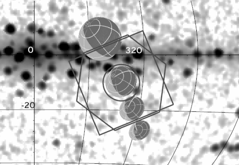
Figure 1: Illustration of the INTEGRAL Earth observing mode. Zero sensitivity FoVs of JEM-X, IBIS and SPI are shown with a circle, box and hexagon respectively superposed on to the RXTE 3-20 keV slew map. In this map many compact sources and extended X-ray emission associated with the Galactic Ridge are visible. In the course of the observation the pointing direction of the telescopes remains the same, while the Earth crosses the instruments FoVs. Day side of the Earth is shown by lighter shade of gray. The linear sizes of the fully coded FoVs are roughly twice smaller. In the course of the observation the Earth moves from positive to negative latitudes. The distance from the Earth increases rapidly during this part of the 3-day INTEGRAL orbit and the angular size of the Earth disk decreases.

2.2 “Background” field

Ideally one would like to observe the Earth modulated CXB signal having an “empty” (extragalactic) field as a background. However due to the requirement of observing the Earth at the beginning of a revolution and the properties of the INTEGRAL orbit the pointing direction of the satellite was set to $l\sim 327$, $b\sim-10$, i.e. rather close to the Galactic plane (Fig.1). As a result the recorded variations of the count rates were not only due to the CXB modulation but also due to occultation of compact sources and the Galactic Ridge emission by the Earth disk. This is further discussed in section 3.7).

The same field has been observed by INTEGRAL multiple times during the regular observational program. Fig.2 shows the 17-60 keV image averaged over multiple observations during several years of INTEGRAL operations (left) and the much less deep image obtained by averaging 4 observations during the Earth observations (right). The list of sources detected with S/N $>4.5\sigma$ during the Earth observation is given in Table 2. One of the sources - IGR J17062-6143 - was found during the Earth observations. The source is apparently a transient, since it is not present in the images averaged over all previous observations. The last column in the table indicates whether the source was obscured by the Earth disk in the course of observations. Further discussion on the contamination of the CXB signal by compact sources is given in section 3.7.

Table 2: The list of compact sources detected during the Earth observations with INTEGRAL. The flux in the 17-60 keV band is quoted. In this band 1 mCrab corresponds to $\sim 1.4\leavevmode\nobreak\ 10^{-11}\leavevmode\nobreak\ {\rm ergs\leavevmode\nobreak\ cm^{-2}\leavevmode\nobreak\ s^{-1}}.$ The new source IGR J17062-6143 was discovered during the Earth observations with INTEGRAL.

Source	Flux,mCrab	S/N	Occult.
GX339-4	$30.9\pm 1.4$	21.6	N
4U1626-67	$12.0\pm 0.7$	16.3	Y
SWIFT J1626.6-5156	$13.9\pm 1.0$	14.3	Y
4U 1538-522	$17.8\pm 1.3$	13.5	Y
IGR J16318-4848	$20.9\pm 1.6$	13.0	Y
4U 1636-536	$6.7\pm 0.8$	8.5	Y
PSR 1509-58	$7.2\pm 1.2$	6.1	N
IGR J17062-6143∗	$3.4\pm 0.6$	5.8	Y
GX 340+0	$60.2\pm 10.4$	5.8	Y
NGC 6300	$3.3\pm 0.6$	5.4	Y
XTE J1701-462	$15.5\pm 3.3$	4.7	N

• ^∗ - newly detected source

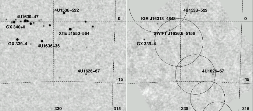
Figure 2: “Background” field: map built using the data averaged over several years (left) and actual image during Earth observations (right). The circles shows the Earth disk during several consecutive moments of time. Darker shades of grey correspond to higher S/N ratio.

2.3 JEM-X

Initial reduction of JEM-X data was done using the standard INTEGRAL Off-line Science Analysis software version 5.1 (OSA-5.1) distributed by the INTEGRAL Science Data Centre. We use the event lists to which, an arrival time, energy gain and position gain corrections have been applied (the so called COR level data in the OSA-5.1 notations). Using these lists the light curves and spectra for the whole detector (i.e. ignoring position information) have been generated. To convert the detector count rates into photon rates we used the Crab nebula observations in revolution number 300, when the Crab was in the center of JEM-X FoV (see more discussion on the cross calibration in Sect. 3.8). For the Earth observations the effective area was calculated over the part of the disk within JEM-X FoV, taking into account position dependent vignetting. In the subsequent analysis we used only the data from JEM-X unit 1 which has a more accurate calibration than unit 2.

Each of the Earth observations started immediately after switching on the spacecraft instruments at the Earth radiation belts exit. The first 4 ksec of each observation were discarded because of the strong variations of the JEM-X gain usually accompanying the instrument turn-on.

Light curves of the JEM-X detector during two observations (revolutions 401 and 406) can be well described in terms of our CXB-modulation model. In other two observations (revolutions 404 and 405) an additional component is clearly present in the detector light curve, which can be interpreted as due to auroral emission from the Earth (see section 3.6). The examples of JEM-X light curves (with and without evidence for auroral emission) are shown in Fig.3. For the CXB analysis we used only the JEM-X data obtained during revolutions 401 and 406 where the contribution from the auroral emission is small (see section 3.6).

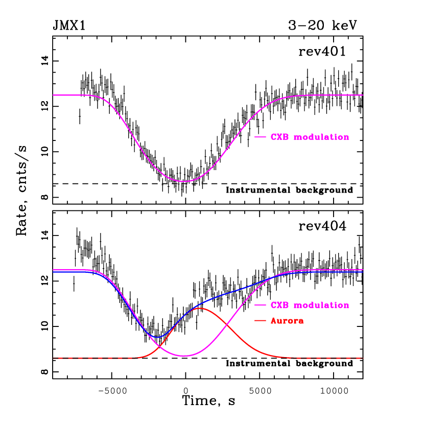
Figure 3: Count rates collected by JEM-X1 detector in the 3-20 energy band during two sets of Earth observations carried out on Jan. 24-25 and Feb. 2-3, 2006 (revolutions 401 and 404 respectively). Solid thick lines show the contribution of CXB flux modulation and the Earth Auroral emission. The auroral model assumes that the emission comes from the circular region with a radius of order of $0.1\times R_{E}$ around the Earth North magnetic pole. Such model is probably too simple to rely upon and the revolutions 404 and 405 (showing clear signs of auroral emission) have been removed from the analysis. Short dashed line shows the instrumental background level. Zero time in these plots corresponds to maximum coverage of the JEM-X FoV by the Earth disk.

2.4 IBIS

For the IBIS/ISGRI data the energies of the events were calculated using the standard conversion tables available in the OSA 5.1 distribution. The secular evolution of the detector gain was corrected using the position of fluorescent line of tungsten at $\sim$60 keV in the detector background spectrum. The count rate for the whole detector in 1 keV wide channels was used for subsequent analysis.

2.5 SPI

SPI spectra in 0.5 keV wide energy bins were accumulated for 200 second intervals from standard energy-calibrated events. Over this time interval, the sky as occulted by the Earth can be assumed to be constant. The light curves measured by each of the 17 detectors of SPI were used (independently) in the subsequent analysis.

2.6 OMC

As explained in Sect. 2.1, the star trackers of the spacecraft were switched off when the Earth limb was at less than 15^∘from the main axis, so that the satellite was passively drifting during the occultation. The Optical Monitoring Camera (OMC) was configured to obtain several reference images of the stellar background before and after the Earth occultation, which could be used as a backup to recover the attitude of the spacecraft if there were any technical problem. OMC obtained a sequence of 13 images of $512\times 512$ pixels (corresponding to 2.5^∘$\times$ 2.5^∘), with integration time of 10 s. The drift measured on the OMC images during the first observation (revolution 401) was $\Delta Y_{sc}=-5.5^{\prime}$ and $\Delta Z_{sc}=+10.9^{\prime}$, totalling 12.2’ in a period of time $\Delta T=06h\leavevmode\nobreak\ 48m\leavevmode\nobreak\ 33s$. $Y_{sc}$ and $Z_{sc}$ are the spacecraft reference axes. This drift is fully consistent with the interpolation of the spacecraft attitude control system data, used to determine the pointing direction. The diffuse light originated by the illuminated fraction of the Earth was detectable by OMC already 1 hour before entering the Earth limb (when the OMC axis was at around 18^∘from the Earth centre). Although the integration time was reduced to 1 s when the Earth was within the OMC field of view, the diffuse light was bright enough to completely saturate the OMC CCD.

3 Methods and analysis

An obvious signature of the Earth obscuration of the CXB in the INTEGRAL data is the characteristic depression in the observed light curves (e.g. Fig.3). This depression to the first approximation reflects variations of the angular size of the Earth as seen by each of the instruments. Unfortunately there are several other variable components contributing to the light curves, which complicate the extraction of the CXB signal. We now discuss all these components and argue that their contribution can be suppressed by filtering the data or can be explicitly taken into account.

3.1 Model components

The total flux $F(E,t)$ measured by the INTEGRAL detectors at a given time $t$ and given energy $E$ can be separated into several components: internal detector background $B(E)$, flux from bright galactic X-ray sources $\sum_{i}F_{S,i}(E,t)$, collective flux from weak unresolved galactic sources (Galactic Ridge) $F_{\rm Ridge}(E,t)$, CXB emission $F_{\rm CXB}(E,t)$, Earth atmospheric emission induced by cosmic ray particles $F_{\rm Atm}(E,t)$, the Earth auroral and day side emission $F_{\rm Aur}(E,t)$, the emission (CXB and galactic sources) reflected by the Earth atmosphere $F_{\rm Refl}(E,t)$. The contributions of these components have to be evaluated with account for the Earth modulation and the effective area of the detectors. Each of the components leaves a specific signature in the detector light curve.

Accordingly we can simply write that the flux is the sum of the above mentioned components:

$$F(E,t)=B(E)+\sum_{i}F_{S,i}(E,t)+F_{\rm Ridge}(E,t)+$$

$$F_{\rm Aur}(E,t)+F_{\rm Atm}(E,t)+F_{\rm CXB}(E,t)+F_{\rm Refl}(E,t).$$ (1)

Here and below we use the notion $F(E)$ for the count rates (in $\rm cnts\leavevmode\nobreak\ s^{-1}\leavevmode\nobreak\ keV^{-1}$) measured by each of the detectors in a given energy bin and $S(E)$ for true spectra (in $\rm phot\leavevmode\nobreak\ s^{-1}\leavevmode\nobreak\ cm^{-2}\leavevmode\nobreak\ keV^{-1}$). The conversion from $S(E)$ to $F(E)$ is the convolution with the effective area, vignetting term, solid angle (for diffuse sources) and the energy response matrix of each detector. For brevity we do not explicitly write the convolution in the subsequent expressions.

3.2 CXB model

The canonical broad band CXB spectrum in the energy range of interest is based on the HEAO-1 data. The following analytic approximation was suggested by Gruber et al. (1999):

$$S^{G99}_{CXB}(E)=\left\{\begin{array}[]{ll}7.877\leavevmode\nobreak\ E^{-0.29}\leavevmode\nobreak\ e^{-E/41.13}&3<E<60\leavevmode\nobreak\ {\rm keV}\\ &\\ 0.0259\leavevmode\nobreak\ (E/60)^{-5.5}+&\\ 0.504\leavevmode\nobreak\ (E/60)^{-1.58}+&E>60\leavevmode\nobreak\ {\rm keV}\\ 0.0288\leavevmode\nobreak\ (E/60)^{-1.05}&\end{array}\right.$$ (7)

Here $S^{G99}_{\rm CXB}(E)$ is in units of ${\rm keV/keV\leavevmode\nobreak\ cm^{-2}\leavevmode\nobreak\ s^{-1}\leavevmode\nobreak\ sr^{-1}}$. Below we use notation $S_{\rm CXB}(E)$ for the (unknown) CXB spectrum to distinguish it from $S^{G99}_{\rm CXB}(E)$ spectrum given by eq.7.

The obscuration of the CXB by the Earth disk produces the depression in the recorded flux with an amplitude set by the surface brightness of the CXB and the solid angle $\Omega(t)$ subtended by the Earth $S_{CXB}(E)\Omega(t)$.

3.3 CXB reflection by the Earth’s atmosphere

The outer layers of the Earth’s atmosphere reflect part of the incident X-ray spectrum via Compton scattering. The picture is very similar to the well studied case of the reflection from a star surface (e.g. Basko, Sunyaev & Titarchuk, 1974) or an accretion disk (e.g. George & Fabian, 1991) except for the different chemical composition of the reflecting medium. The spectrum reflected by the Earth’s atmosphere was calculated (Churazov et al., 2006) using a Monte-Carlo method for a realistic chemical composition of the atmosphere and taking into account all relevant physical processes (photoabsorption, Compton scattering and Rayleigh scattering on the electrons bound in the molecules and atoms). The reflection is most significant near $\sim$60 keV and declines towards lower or higher energies (see Fig.4).

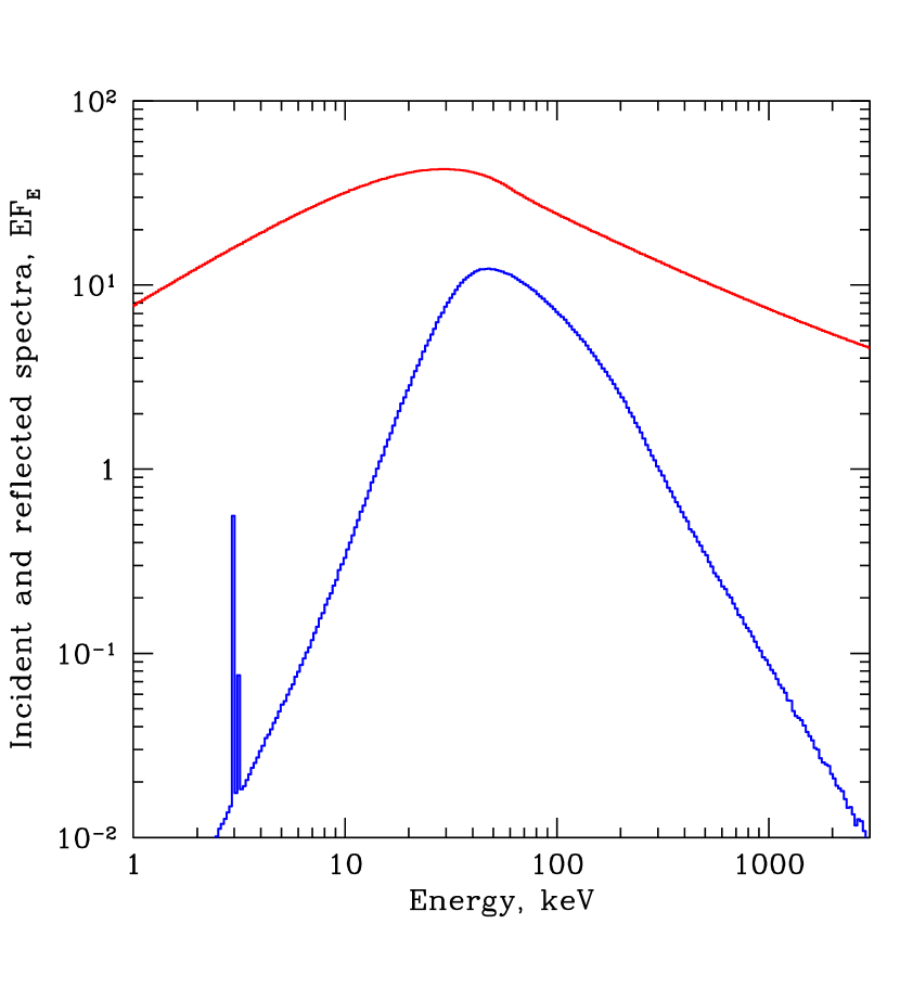
Figure 4: The CXB spectrum and the spectrum reflected by the Earth atmosphere (Churazov et al., 2006). The reflected spectrum was integrated over all angles. The features in the reflected spectrum near 3 keV are the fluorescent lines of argon. The approximation of the albedo given in eq. 8 neglects the flourescent lines.

The ratio of the reflected and incident spectra (energy dependent albedo $A(E)$) was evaluated for the CXB spectrum shape measured by HEAO-1 (eq.7) and approximated by the following expression (eq.6 of Churazov et al. 2006):

$$A(E)=\frac{1.22}{\left(\frac{E}{28.5}\right)^{-2.54}+\left(\frac{E}{51.3}\right)^{1.57}-0.37}\times$$

$$\frac{2.93+\left(\frac{E}{3.08}\right)^{4}}{1+\left(\frac{E}{3.08}\right)^{4}}\times$$

$$\frac{0.123+\left(\frac{E}{91.83}\right)^{3.44}}{1+\left(\frac{E}{91.83}\right)^{3.44}}$$ (8)

For an observer located at some distance $D$ from the Earth the flux integrated over the full Earth disk will then be:

$$F_{\rm Albedo}(E)=S_{CXB}(E)A(E)\Omega(t),$$ (9)

Strictly speaking the factorization of the reflected spectrum into the product of the incident spectrum and the energy dependent albedo is valid only if $A(E)$ was calculated for a spectrum having the same spectral shape as $S_{CXB}(E)$. In practice the albedo is not strongly sensitive to the assumed shape of the incident spectrum (see Churazov et al., 2006 for details). Much of our results (see below) were obtained assuming that $S_{\rm CXB}=\beta\leavevmode\nobreak\ S^{G99}_{\rm CXB}(E)$ which makes the expression (9) exact. Here $\beta$ is the normalization constant, independent of energy. The angular dependence of the emerging spectra is not important as long as the full Earth disk is used (see Churazov et al., 2006). In particular the result does not depend on the distance $D$ from the Earth. If however only a part of the disk is seen or if the effective area of the telescope varies substantially across the Earth disk, then the albedo is no longer described by a universal function and has to be calculated taking into account the angular dependence of the emerging radiation. For IBIS and SPI instruments with wide FoVs this simple approximation may fail only for the very beginning (few ksec) or the very end of each observation when only fraction of the disk is seen (Fig.1). As is discussed further in section 3.7 the data during first 5 ksec of each observation have been discarded anyway. At the end of each observation the effect is small, since the Earth has much smaller angular size and vignetting near the zero sensitivity FoV edge further suppresses the signal. JEM-X has narrower FoV, but the contribution of the reflection is small in the JEM-X energy range. Thus the modulation of the CXB flux by the Earth (depression in the light curve) observed by the instruments can be written as:

$$F_{\rm CXB}(E,t)=S_{\rm CXB}(E)[1-A(E)]\Omega(t).$$ (10)

Since the outer layers of the Earth atmosphere may be opaque at low energies and transparent at high energies the apparent angular “size” of the Earth $\Omega$ (see eq.10) does depend on energy. For instance at 1 keV the optical depth reaches unity for a line of sight having an impact parameter of $\sim R_{e}+$ 120 km, where $R_{e}$ is the Earth radius. For comparison at 1 MeV the corresponding impact parameter is $\sim R_{e}+$ 70 km. This effect limits the accuracy of the above approximation - eq.10 - to $\sim$1-2%.

3.4 Earth X-ray albedo due to Galactic sources

The Earth atmosphere will also reflect X-rays from the Galactic sources. Since the pointing direction is in the general direction of the Galactic Center, most of the Galactic bright sources are located “behind” the Earth and their reflected emission does not contribute to the flux measured by INTEGRAL. One can therefore expect that the Crab nebula, located at the Galaxy anti-center will be the dominant source of the contamination. An easy estimate of this contamination can be done simply by calculating the total incident flux of the CXB and Crab emission coming on to a side of the Earth towards the observer. If we assume that the intensity of the CXB at the energy of $\sim$ 30 keV is $\sim 1.8$ mCrab per square degree, and we integrate over all incidence angles, we obtain an estimate of the total incident CXB flux per 1 ${\rm cm^{2}}$ of the atmosphere of $\sim$ 19 Crab. Thus for one hemisphere the ratio of total incident CXB and Crab fluxes is $\frac{19\times 2\pi R_{e}^{2}}{\pi R_{e}^{2}}\sim 40:1$. The maximal value of the albedo is of the order of 35%. Therefore the contribution of the Crab emission reflected by the Earth atmosphere can be roughly estimated to be at the level of $35\%/40\sim$1% relative to the CXB signal. In the subsequent analysis we neglect this component.

3.5 Earth atmospheric emission

Due to the bombardment by cosmic rays, the Earth’s atmosphere is a powerful source of hard X-ray and gamma-ray emission. Although experimental and theoretical studies of this phenomenon have a long history starting in the 1960s, there remains a significant uncertainty with regard to the emergent spectrum of the atmospheric emission, in particular in the energy range of interest to us – between 10 and 200 keV. On the other hand, the hadronic and electromagnetic processes responsible for the production of atmospheric emission, although complicated, are well understood. Similarly, the incident spectrum of cosmic rays has been recently measured with high precision. This implies that with the power of modern computers, the spectrum and flux of atmospheric X-ray emission should be predictable by simulations to a reasonable accuracy. We performed such a numerical modeling using the toolkit Geant 4. A detailed report on our analysis and results is presented elsewhere (Sazonov et al. 2006). Here we briefly summarize the main outcome of our simulations.

We found that at the energies of interest to us, most of the emerging X-ray photons have almost no memory of their origin, i.e. they were produced (mainly by bremsstrahlung and positron–electron annihilation) with relatively high energy at a significant atmospheric depth (several grams or tens of grams of air per sq. cm from the top of the atmosphere) and escaped into free space after multiple Compton down-scatterings.

This process is similar to the formation of supernova hard X-ray spectrum resulting from down Comptonization of ⁵⁶Co gamma ray lines in an optically thick envelope. Such a spectrum was observed from SN1987A (Sunyaev et al. 1987)

As a result, the emergent spectrum (see Fig.5) is barely sensitive to the energy of the parent cosmic ray particle (in the relevant range from a fraction of 1 GeV to a few hundred GeV) or to the type of the incident particles (e.g. proton, alpha-particle, electron). In the energy range 25–300 keV the emergent spectrum is well fitted with the following formula (Sazonov et al., 2006):

$$S_{ATM}(E)=\frac{C}{(E/44)^{-5}+(E/44)^{1.4}}$$ (11)

The photon spectrum peaks around 44 keV. At energies below the maximum the spectrum shows a rapid decline (as $E^{-5}$) due to photoabsorption. Since the emission is already very low at 25 keV, we did not try to approximate the spectrum below this energy (where the shape is noticeably different). Above $\sim 300$ keV the spectrum starts to be dominated by the comptonization continuum associated with the prominent 511 keV annihilation line and the approximation given by equation (11) again breaks down.

The work of Sazonov et al. (2006) also predicts the normalization $C$ of the atmospheric emission spectrum as function of the solar modulation parameter and the rigidity cut-off associated with the Earth’s magnetic field. The cut-off is calculated in the shifted dipole approximation, with Stoermer’s formula. For the specific conditions of the INTEGRAL observations, the predicted brightness of the atmospheric emission is 31.7 ${\rm keV^{2}\leavevmode\nobreak\ cm^{-2}\leavevmode\nobreak\ s^{-1}\leavevmode\nobreak\ keV^{-1}\leavevmode\nobreak\ sr^{-1}}$. This value was obtained by averaging the brightness of the atmosphere over the Earth disk and adopting the solar modulation parameter $\phi=$0.45 GeV, corresponding to the dates of the observations (see Sazonov et al. 2006 for details). This value will be compared with that inferred from our fitting procedure of the measured spectrum in Section 4.

Figure 5: Examples of simulated spectra (solid lines) of atmospheric emission produced by cosmic protons of given energy: $E_{p}=$ 1, 10 and 100 GeV. It can be seen that in the photon energy range 25-300 keV the shape of the emergent spectrum is almost invariant and well fitted with eq.11 (the dashed lines).

3.6 Earth Auroral and day-side emission

As mentioned above not all JEM-X observations can be well described by a simple model of the CXB signal modulated by the Earth. In the revolutions 404 (see Fig.3, bottom panel) and 405 the light curves clearly deviate from the prediction of the pure CXB modulation model. The excess in the light curve appeared when a large part of the field of view was covered by the Earth disk. This suggests that there is an additional source of the X-ray emission in the direction of the Earth. The most plausible explanation of this excess is the Earth auroral emission. We then added to our CXB-modulation model an additional component, assuming that the emission comes from the circular region with a radius of order of $0.1\times R_{E}$ around the Earth North magnetic pole. This two-component model provides a reasonable description of the data (see Fig.3), thus broadly supporting the auroral origin of the emission. However the observed light curve in revolution 404 (Fig.3, bottom panel) suggests that a more complicated model of auroral emission is needed. We therefore decided to limit the analysis of the JEM-X data to revolutions 401 and 406 which are not affected by the auroral emission.

During our observations the Earth disk was predominantly dark (see Fig.1). The emission from the dark side (induced by the cosmic rays bombardment) is discussed in section 3.5). The day side of the Earth is a source of additional X-ray emission due to the reflection of Solar flares and non-flaring corona (e.g. Itoh et al. 2002). This emission is typically very soft and is not important at energies higher than a few keV. In principle, an increased hard X-ray flux from dayside Earth might be expected at the time of powerful Solar flares, but monitoring of the Solar activity (http://www.sec.noaa.gov) did not show any significant Solar flares during our observations. In the subsequent analysis we have neglected the Earth day side emission.

3.7 Compact sources and the Galactic ridge

As was already mentioned above both relatively bright compact sources, which are detectable with INTEGRAL and unresolved Galactic emission (Galactic Ridge) have to be removed from the data in order to get a clean estimate of the CXB flux.

Bright compact sources can be detected directly by INTEGRAL telescopes, and their contribution can be subtracted from the detector’s count rate. However this procedure would increase the statistical errors of the CXB flux measurements, especially if a large sample of compact sources is considered.

Contribution of the unresolved Galactic background (Galactic ridge emission) can be estimated using the results of Revnivtsev et al. (2006) and Krivonos et al. (2007). There it is shown that the Galactic ridge X-ray emission surface brightness correlates very well with the Galactic near-infrared surface brightness. Using data of COBE/DIRBE (LAMBDA archive , http://lambda.gsfc.nasa.gov/) and correlation coefficients from Krivonos et al. (2007) we obtained that the peak surface brightness of the Galactic ridge at Galactic longitude $l\sim 330$ is approximately $\sim 1$ mCrab/deg² in the energy band 17-60 keV, providing approximately $\sim 20-30$ mCrab net flux for IBIS/ISGRI and SPI. Thus the contribution of the Galactic Ridge can be modeled using the near-infrared data, convolved with the angular response of the INTEGRAL instruments.

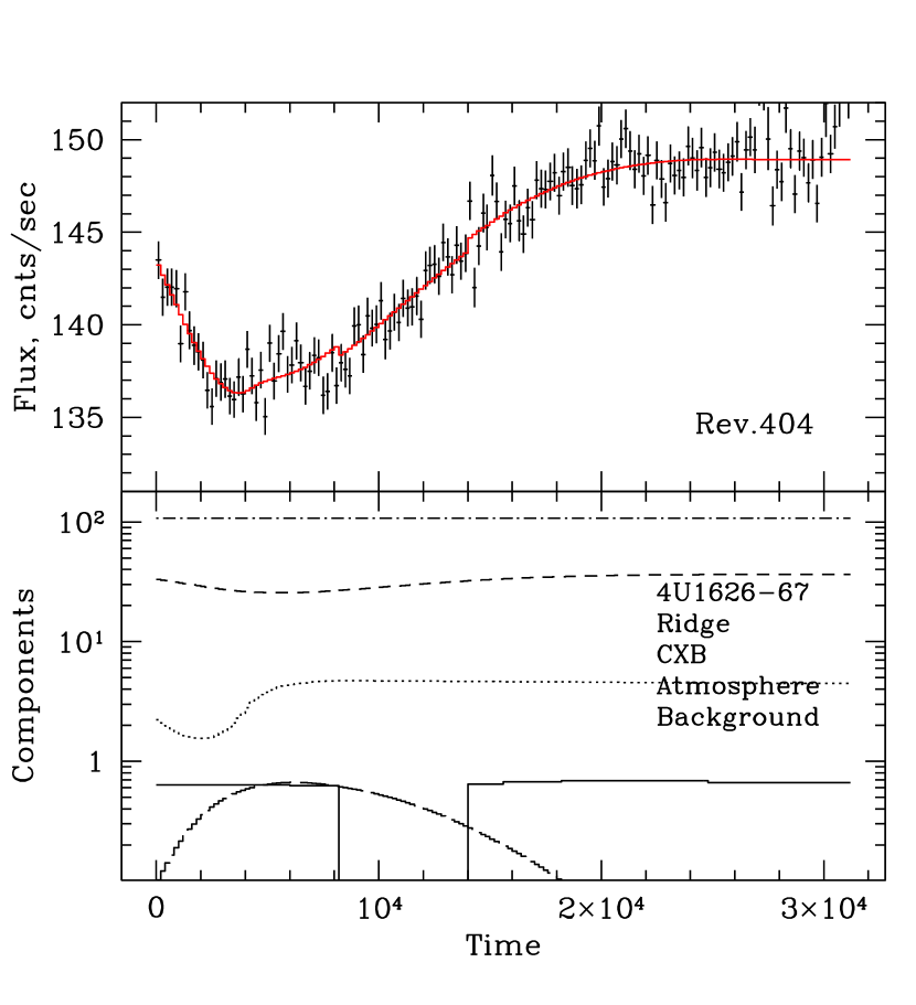
Figure 6: Illustration of the various components contributing the the IBIS/ISGRI light curve in the 20-40 keV band. Upper panel: total count rate in the 20-40 keV band together with the best-fit model (solid curve). Lower panel: model components: internal detector background (dash-dotted line), CXB emission (short-dash line), Galactic Ridge emission (dotted line), the Earth atmospheric emission (long-dash line) and a single compact source 4U1626-67 (solid line). The normalizations of these components were free parameters of the model. The CXB flux, modulated by the Earth disk, is the main source of the flux variations observed by INTEGRAL instruments. The internal detector background is assumed to be stable. The Galactic Ridge crosses the edge of the IBIS field of view and the Earth blocks the ridge emission only during first 3-4 ksec of the observation (see Fig.1). Both CXB obscuration and the Earth atmospheric emission reach the maximum amplitude approximately 6 ksec after the start of the observation, when the Earth disk has still a large angular size and fills the central, most sensitive, part of the FoV.

A typical time dependence of the various components contributing to the A typical time dependence of the various components contributing to the total count rate of IBIS/ISGRI is illustrated in Fig.6. In the upper panel the total count rate in the 20-40 keV band is shown together with the best-fit model. The 5 model components, used in this illustration, are shown in the lower panel: internal detector background, CXB emission, Galactic Ridge emission, the Earth atmospheric emission and a single compact source 4U1626-67. The normalizations of each of these components were free parameters of the model. Notice that since the surface brightness of the Galactic Ridge drops sharply towards higher latitudes, this component is affecting only the first few ksec of data. As one can see from Fig.1 and 2 many compact sources are clustered near the Galactic Plane, sharing the same area as the Galactic Ridge. Adding the contributions of the Ridge and several compact sources as independent components would make the task of separating them very difficult. In order to make the analysis more robust we decided to cut out the first $\sim$ 5 ksec of data (when the Ridge contribution is not negligible) from further analysis as shown in Fig.7. This also removes much of problems with the occultation of compact sources, located near the Plane. The only moderately strong source located far above the Galactic plane is 4U1626-67. Inclusion/exclusion of this source in the model changes the net 20-40 keV CXB flux by $\sim 2$%. Therefore with the above data selection all compact sources can be dropped from the model without much impact on the final CXB spectra. Note that JEM-X has smaller field of view, which does not cover the Galactic plane. The brightest source in JEM-X field of view – 1H1556-605 has a mean flux 5-7 mCrab in JEM-X energy band and it is very far from the center of the instrument field of view ($\sim 5.6^{\circ}$) where the effective area of the instrument drops to less than 5% of the maximum. The estimated count rate which might be caused by this source is below the Poisson noise of the detector. Therefore the data cut used for JEM-X is mainly driven by the stability of the internal detector characteristics (see section 2.3).

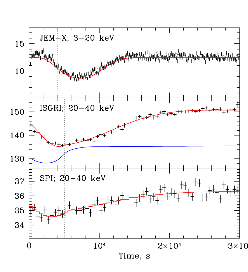
Figure 7: The light curves of JEM-X, IBIS/ISGRI and SPI instruments in units of counts per second. In the middle panel the blue curve shows schematically (with arbitrary normalization) the time dependence of the Galactic Ridge emission, modulated by the Earth occultation. In order to avoid contamination of the CXB measurements due to Galactic plane contribution the first few ksec of data (on the left from the vertical lines) were dropped from the analysis. Note that for JEM-X less strict cut was applied, since its field of view is smaller than that for the other instruments (see section 2.3).

3.8 Instruments absolute and cross- calibration

CXB absolute flux measurements were done several times over the past three decades (see e.g. Horstman-Moretti et al. 1974; Mazets et al. 1975; Kinzer, Johnson, & Kurfess 1978; Marshall et al. 1980; McCammon et al. 1983; Kinzer et al. 1997; Vecchi et al. 1999; Gruber et al. 1999; Kushino et al. 2002; Lumb et al. 2002; Revnivtsev et al. 2003, 2005; Hickox & Markevitch 2006). The reported fluxes show considerable scatter, part of which is likely related to the problem of the absolute flux calibration of the instruments. The same problem appears when the fluxes of the Crab nebula (assumed to be a “standard candle”) derived by different instruments are compared (e.g Toor & Seward 1974; Seward 1992; Kuiper et al. 2001; Kirsch et al. 2005). Therefore in order to make a fair comparison of the CXB spectrum obtained by different instruments one has to make sure that the same assumptions on the “standard candle” (Crab) spectrum are made.

We analyzed several Crab observations with INTEGRAL exactly in the same way as we did for the Earth observations. In particular the revolutions 170 and 300 were used. During these revolutions a large number of observations was performed with the source (Crab) position varying from almost on-axis to essentially outside the field of view. The light curves in narrow energy bands were constructed, together with the predicted signal (based on the source position and the IBIS/ISGRI and SPI angular responses). The intrinsic detector background was added as an independent component to the model (single component for IBIS/ISGRI and 17 independent components for the 17 SPI detectors). The internal background was assumed to be constant with time. The Crab spectrum in counts/sec was derived from the best-fit normalization of the model in each energy bin. For illustration the comparison of the predicted and observed 20-40 keV fluxes in individual (few ksec long) observations during revolution 170 is shown in Fig.8. Comparison of the spectra obtained in revolutions 170 and 300 shows very good agreement between the resulting spectra. Since the set of Crab positions in these two revolutions were different we concluded that our model is providing robust resulting source spectra when a large number of quasi-random source positions is used. This kind of analysis is very similar to the analysis of CXB occultation by the disk of the Earth and it is therefore possible to use the derived raw Crab spectra for calibration/cross-calibration purposes.

Figure 8: Comparison of the predicted and observed 20-40 keV fluxes in individual (few ksec long) observations during revolution 170. The model included two components: constant in time detector background and the predicted signal based on the source position in the IBIS/ISGRI field of view.

Most of the historic measurements of the Crab spectrum (the pulsar plus nebulae) suggest that a single power law is a reasonable approximation below $\sim$100 keV (e.g Toor & Seward 1974; Seward 1992; Kuiper et al. 2001; Kirsch et al. 2005) with the scatter in the reported values of the photon index of $\sim$0.1 (see Fig.9). The reported fluxes also show considerable scatter (Table 3). While the accurate absolute measurements of the Crab spectrum are of profound importance for the X-ray astronomy, for our immediate purposes the crucial issue is to use the same definition of the “standard candle” for all instruments to allow for a fair comparison of the CXB signal. The basic assumption here is that the intrinsic variability of the Crab is small compared to the required level of accuracy.

We choose the Crab spectrum in the form $dN/dE=10\leavevmode\nobreak\ E^{-2.1}$ phot s^-1 cm^-2 keV^-1. This simple approximation provides a reasonable compromise among historic Crab observations in terms of the spectral slope and flux in the energy range of interest (see Fig.9 and Table 3). We then cross-calibrated the INTEGRAL instruments (using the spectra extracted with the above mentioned procedure) to ensure that the reference Crab spectrum is recovered. Since the slope of CXB is not dramatically different from the Crab spectrum near the energy of the maximum energy release, one can do this procedure by introducing a special fudge factor (a smooth function of energy) such that the raw spectra in counts divided by the effective area with this fudge factor recover the assumed Crab spectrum in phot s^-1 cm^-2 keV^-1. While this approach has obvious limitations and disadvantages its simplicity and robustness fits well the purposes of this particular work (at least in the first approximation).

Thus, in our subsequent analysis we assume that the shape of the Crab nebula spectrum in the energy band 5-100 keV is described by a power law $dN/dE=10\leavevmode\nobreak\ E^{-2.1}$ phot s^-1 cm^-2 keV^-1. Any changes in the assumed Crab normalization and in the spectral shape can then be easily translated into changes in the CXB spectrum. While reasonable, this choice of the Crab spectrum is still arbitrary and one has to bear this in mind when making the comparison with the results of other mission. An assumption that any of the values quoted in Table 3 have equal likelihood of being the closest approximation to the true (unknown) flux from the Crab implies the uncertainty in absolute flux calibration can be as high as $\sim$30% (e.g. flux measured by GRIS), although majority of points come within $\pm$10% of the value adopted here. A more fair relative comparison is possible only if the measured CXB flux is quoted together with the measured Crab flux in the same energy band.

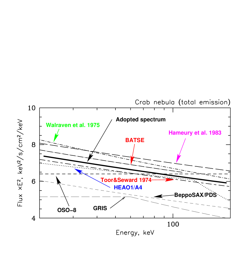
Figure 9: Best-fit spectra of the Crab nebula (total emission) measured by different experiments in the hard X-ray band. The spectrum adopted here is shown with the thick solid line.

Table 3: Crab nebula fluxes in the 20-50 keV energy band, measured by different experiments. The value adopted for this paper is shown in bold face.

Measurements	Flux 20-50 keV
	$10^{-9}$erg s-1 cm-2
Rockets(Toor & Seward 1974)	10.0
Rocket(Walraven et al. 1975)	11.2
OSO-8 (Dolan et al. 1977)	9.4
Hameury et al. (1983)	11.3
HEAO1/A4(Jung 1989)	9.8
GRIS(Bartlett 1994)	7.6
CGRO/BATSE(Ling & Wheaton 2003)	10.8
BeppoSAX/PDS(Kirsch et al. 2005)	8.6
RXTE/HEXTE(Kirsch et al. 2005)	10.6
Adopted here $dN/dE=10\leavevmode\nobreak\ E^{-2.1}$	10.4

3.9 CXB cosmic variance

The total CXB flux due to unresolved sources within the given area of sky may vary due to Poissonian variations of the number of sources, intrinsic variability of the source fluxes or due to the presence of a large scale structure of the Universe (see e.g. Fabian & Barcons 1992). The number counts of extragalactic sources at about the flux level corresponding to the INTEGRAL instruments sensitivity ($f_{\rm x}\sim 10^{-11}$ erg s^-1cm^-2 in the 20-50 keV band) is consistent with a power law having a slope $\alpha=-1.5$ and normalization $\sim 1.4\times 10^{-2}$ deg^-2 (Krivonos et al. 2005). The effective size of the region of sky occulted by the Earth during INTEGRAL observations is $\sim 10\times 15$ degrees (visible diameter of the Earth times the length of the path the Earth center makes in the sensitive part of the FOV). In this case expected Poissonian variations of the CXB flux due to unresolved extragalactic sources are smaller than 1%. This estimate assumes that sources with a flux $>10^{-11}$ erg s^-1 cm^-2 would be detected and accounted for. A similar estimate can be obtained by rescaling the RXTE/PCA 3-20 keV measurement of the CXB variations at 1^∘ angular scale (Revnivtsev et al. 2003) to a larger area.

The variance of the CXB originating from large scale structure of the local Universe was extensively studied using the HEAO-1 data (e.g. Shafer & Fabian 1983; Miyaji et al. 1994; Lahav, Piran, & Treyer 1997; Treyer et al. 1998; Scharf et al. 2000). The largest scale anisotropy (dipole component) is approximately consistent with Compton-Getting effect due to the motion of the Earth with respect to the Cosmic Microwave Background rest frame. However some additional dipole anisotropy was suggested, which is consistent with the predicted large-scale structure variations (e.g Treyer et al. 1998; Scharf et al. 2000). It was shown that in total these variations are at the level of $\sim 0.5$%. At smaller angular scales the amplitude of the variations due to large scale structure is rising but at the angular scales $\sim 10^{\circ}$ it should not exceed $\sim$1% (e.g. Treyer et al. 1998). Summarizing all of the above one can conclude that for a region of sky used for a determination of the CXB spectrum during the INTEGRAL observations (effective size of the order of $10\times 10$ degrees), the CXB cosmic variance is becoming a limiting factor at a level of accuracy of $\sim$1%.

4 Results

As discussed in the previous section after the data filtering only 4 components are left in the model: the intrinsic detector background, the modulation of the CXB signal, the CXB radiation reflected by the Earth and the Earth atmospheric emission. All these components primarily depend on the solid angle (within the FOV) subtended by the Earth. To evaluate the impact of each of these components on the observed light curves one has to average the signals over the Earth disk, taking into account the effective area of the telescopes. E.g. for the atmospheric emission the signal was averaged taking into account rigidity distribution, angular distribution of the emerging atmospheric emission and the telescopes vignetting. After such averaging the CXB flux modulation (including Compton reflection) and the flux variations due to the Earth atmospheric emission produce very similar signatures (but with the opposite signs) in the detector light curves. This severely complicates any attempts to disentangle these contributions directly from the observed light curves. Instead it was assumed that a combination of these components can be described as a single time dependent signal for each measured energy bin:

$$F(E,t)\approx C(E)-S_{\rm CXB}(E)\left[1-A(E)\right]\Omega(t)+$$

$$S_{\rm ATM}(E)\Omega(t)=C(E)-S_{\rm Earth}(E)\Omega(t),$$ (12)

where $S_{\rm ATM}(E)$ is the spectrum of the cosmic ray induced atmospheric emission (averaged over the Earth disk and normalized per unit solid angle), and $S_{\rm Earth}(E)=S_{\rm CXB}(E)\left[1-A(E)\right]-S_{\rm ATM}(E)$ is the combined flux of all components related to the presence of the Earth in the FoV. A constant in time $C(E)$ includes the intrinsic background and total combined flux of Galactic sources and CXB without the Earth in the field of view. Using the observed light curves $F(E,t)$ in each energy bin and the known effective solid angle $\Omega(t)$ subtended by the Earth in the FoV of each instrument the $F_{\rm Earth}(E)$ counts spectra (i.e. $S_{\rm Earth}(E)$ convolved with the effective area and the energy redistribution matrix) were obtained. As an example the counts spectrum $F_{\rm Earth}(E)$ for SPI is shown in Fig.10. In the right panel of Fig.10 the components of the model spectrum $S_{\rm Earth}(E)$ (CXB spectrum, CXB spectrum corrected for the Compton reflection and for the Earth atmospheric emission) are shown.

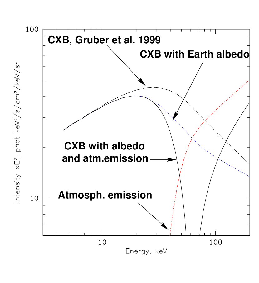
Figure 10: Left – the $F_{\rm Earth}(E)$ spectrum obtained by INTEGRAL/SPI. The dashed line shows the CXB model spectrum. The dotted line shows the same spectrum modified by the Earth albedo. The solid line show the expected spectrum corrected also for atmospheric emission. Right – theoretical models of the same spectral components, used in the left figure: CXB spectrum, CXB spectrum corrected for albedo. In addition the atmospheric emission emission spectrum is also shown (the dashed-dotted line). Note that the CXB and the atmospheric emission components contribute to the observed spectrum with different signs and the total signal (CXB with albedo and atmospheric emission) changes sign between 60 and 70 keV.

The observed spectrum was fitted in XSPEC (e.g.Arnaud 1996) with a 3-component model, which includes: i) the CXB spectrum in the form of eq.(7) with free normalization, ii) a fixed multiplicative model describing reflection of the CXB from the Earth atmosphere according to eq.(8,10), and iii) the Earth atmospheric emission in the form of eq.(11) with free normalization. The best-fit provides us two parameters of the model: the normalization of the CXB spectrum and the normalization of the Earth atmospheric emission. The CXB spectrum as measured with INTEGRAL is shown in Fig.11. The data points shown in this figure were obtained from the observed spectra in counts/s by subtracting the best-fit atmospheric emission component, correcting for the Compton reflection and for the effective area. For comparison the reference CXB model spectrum is shown with the dashed line, with the absolute normalization increased by 10% compared to eq.7. There is a reasonable agreement between the data and the renormalized CXB spectrum. More sophisticated models are not required by the present data set. Below $\sim$10-20 keV extended data sets, available from other observatories (e.g. RXTE), provide better constraints on the CXB shape than INTEGRAL. More relevant for INTEGRAL observations is the consistency of the CXB spectrum approximation on the energies above 30 keV, i.e. above the energy of the CXB peak luminosity. Considering only the data in the 40-200 keV range and approximating the spectrum with a power law one gets the photon index of 2.42$\pm$0.4. For comparison, the CXB spectrum measured by HEAO-1 (Gruber et al. 1999) can be characterized by a photon index $\sim$2.65 in the same range. If errors scale roughly as square root of time then $\sim$4 times longer data set will be required to bring the uncertainty in the photon index to $\sim 0.2$. Note that these estimates are based on the assumption that the shape of the atmospheric emission is accurately predicted by simulations. Further observations during different phase of the Solar cycle would be very instrumental in proving this assumption.

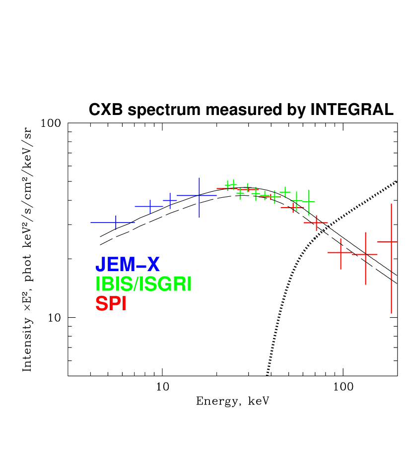
Figure 11: Spectrum of the CXB measured by INTEGRAL instruments. The error bars plotted account for the uncertainties in the normalization of the atmospheric emission component. The dashed line shows the analytic approximation of the CXB spectrum by Gruber et al., 1999. The solid line shows the same spectrum with the best-fit normalization obtained in this work. The thick dotted line shows the best-fit spectrum of the Earth atmospheric emission.

Using the accurate measurement of the cosmic ray spectra and detailed simulations (Sazonov et al., 2006) one can make an accurate prediction of the atmospheric emission. In the present analysis we treat the normalization of this component as a free parameter of the model. The best-fit normalization of this component obtained in present analysis is $32.9\pm 1.3$ ${\rm keV^{2}cm^{-2}s^{-1}keV^{-1}sr^{-1}}$ which agrees well with the expected value of $31.7$. This excellent agreement is encouraging. We note however that the normalization of this component is subject to the same systematic uncertainties associated with the absolute flux calibration discussed above. Further observations with INTEGRAL (with a different seasonal modulation of the cosmic ray spectrum) would be useful to verify the agreement of observations and predictions. Potentially the atmospheric emission could become a useful absolute calibrator for the instruments operating in the hard X-ray/gamma-ray bands.

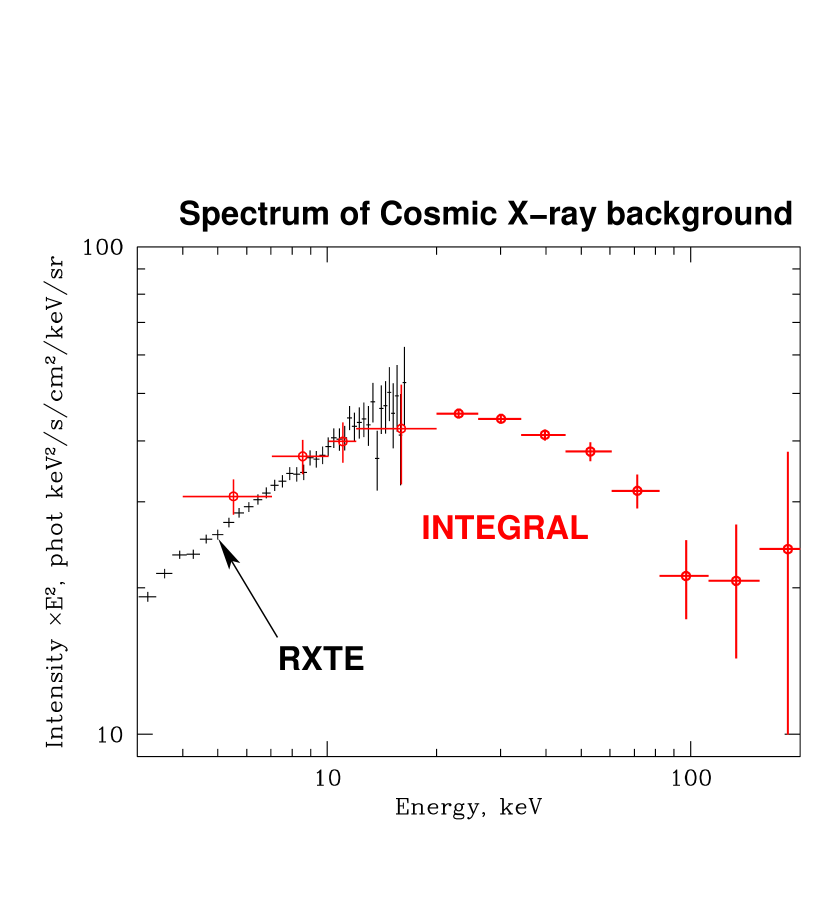
Figure 12: Comparison of the CXB spectrum derived by INTEGRAL with the 3-20 keV CXB spectrum derived from the RXTE data (Revnivtsev et al. 2003). The IBIS/ISGRI and SPI data points were averaged in this plot.

In order to test the sensitivity of the results to the assumed shape of the Crab spectrum, we repeated the same analysis varying the assumed Crab photon index by $\pm 0.1$ (keeping the 20-50 keV flux unchanged) and making appropriate changes in the efficiency fudge factors. The resulting best-fit normalization of the CXB component changed by $\pm\sim$1.2%. This is of course an expected result, given that the assumed 20-50 keV flux from the Crab nebula was unchanged.

We now summarize the uncertainties in the derived CXB normalization. A pure statistical error (joint fit to JEM-X, IBIS/ISGRI and SPI data) in the normalization of the CXB component is $\sim$1%. Further uncertainties are: neglected contributions from compact sources $\leq$2%, modeling the atmospheric reflection $\sim$1-2%, uncertainty in the Crab photon index $\sim$1%. On top of these uncertainties, which if added quadratically amount to $\sim$3%, comes the absolute flux calibration. From the comparison of the Crab 20-50 keV flux measurements (Table 3) it is clear that this is by far the largest source of uncertainty. In particular, as is mentioned above the flux measured by INTEGRAL at $\sim$30 keV is $\sim$10% higher than the value predicted by the fit of Gruber et al., 1999. If we adopt the 20-50 keV Crab flux measured by HEAO-1/A4 (Jung, 1989, see Table 3) and rescale the INTEGRAL measurement accordingly, this difference will shrink to $\sim 4$%.

In Fig.12 we plot the INTEGRAL data together with the CXB spectrum in the 3-20 keV derived from the RXTE data (Revnivtsev et al. 2003). The RXTE data points are above the fit by Gruber et al.(1999), and are derived using a Crab spectrum as $dN/dE=10.8\leavevmode\nobreak\ E^{-2.1}$ phot s^-1 cm^-2 keV^-1 in the 2-10 keV band, i.e. 8% higher than is adopted in this paper. Recent re-analysis of the HEAO-1 A2 data (Jahoda et al., 2007) gives the 2-10 CXB flux $\sim$ 10% lower than the RXTE data points shown in Fig.12. At the same time the most recent Chandra measurements (Hickox & Markevitch, 2006) yields the 2-8 CXB flux higher (but consistent with 1$\sigma$) than the RXTE flux of Revnivtsev et al., 2005. Clearly at present the absolute flux calibration of the instruments (both in the standard 2-10 and hard 20-100 keV X-ray bands) is the dominate source of uncertainties/discrepancies in the CXB measurements.

5 Conclusions

Using the modulation of the aperture flux by the Earth disk, the INTEGRAL observatory measured the spectrum of the cosmic the X-ray background in the energy range $\sim$5-100 keV. The observed flux near the peak of the CXB spectrum (in the $\nu F_{\nu}$ units) at 29 keV is 47 ${\rm keV^{2}cm^{-2}s^{-1}keV^{-1}sr^{-1}}\pm 0.5\leavevmode\nobreak\ (\pm 1.5)$. The qouted uncertainties are pure statistic errors and (in parentheses) systematic errors, excluding the uncertainty associated with the choice of the model Crab spectrum. This value is $\sim$10% higher than suggested by Gruber et al., 1999. Note that in the present analysis the absolute flux calibration was done assuming that the spectrum of the Crab nebula in the relevant energy band is described by the expression $dN/dE=10\leavevmode\nobreak\ E^{-2.1}$ phot s^-1 cm^-2 keV^-1. Any changes in the CXB normalization directly translates into the changes in the energy release by the supermassive black holes in the Universe. These numbers are important for estimating the radiative efficiency of the growing black holes.

In the present analysis the observed level of the atmospheric emission was found to be very close (within 10%) to the results of the simulations. Since accurate measurements of the cosmic ray spectra are now available the Earth atmospheric emission could become a useful “calibration” source for the instruments operating in the few hundred keV range.

The present observations were made during Solar minimum when the expected level of the atmospheric emission (due to cosmic rays interactions with the atmosphere) is close to the maximum. The “background” field was close to the Galactic Plane and part of the data was discarded to avoid contamination of the signal by Earth obscuration of the unresolved Galactic sources. Future (longer) observations during Solar maximum and with the pointing direction away from the Galactic Plane would be very useful to verify the robustness of the atmospheric emission simulations and to obtain the CXB spectrum in broader energy range.