The X-ray binary 2S0114$+$650$=$LSI$+$65 010

Abstract

Context. The X-ray source 2S0114+650$=$LSI$+$65 010 is a binary system containing a B-type primary and a low mass companion believed to be a neutron star. The system has three reported periodicities: the orbital period, P${}_{orb}\sim$11.6 days, X-ray flaring with P${}_{flare}\sim$2.7 hours and a “superorbital” X-ray periodicity P${}_{super}=$30.7 days.

Aims. The objective of this paper is to show that the puzzling periodicities in the system may be explained in the context of scenarios in which tidal interactions drive oscillations in the B-supergiant star.

Methods. We calculate the solution of the equations of motion for one layer of small surface elements distributed along the equator of the star, as they respond to the forces due to gas pressure, centrifugal, coriolis, viscous forces, and the gravitational forces of both stars, which provides variability timescales that can be compared with those observed for 2S0114$+$650. In addition, we use observational data obtained at the Observatorio Astronómico Nacional en San Pedro Mártir (OAN/SPM) between 1993-2004 to determine which periodicities may be present in the optical region.

Results. The models for circular orbits predict “superorbital” periods while the eccentric orbit models predict strong variations on orbital timescales, associated with periastron passage. Both also predict oscillations on timescales of $\sim$2 hrs. We suggest that the tidal oscillations lead to a structured stellar wind which, when fed to the neutron star, produces the X-ray modulations. The connection between the stellar oscillations and the modulation of the mass ejection may lie in the shear energy dissipation generated by the tangential motions that are produced by the tidal effects, particularly in the tidal bulge region. From an observational standpoint, we find indications for variability in the He I 5875 Å line on $\sim$2 hrs timescale and, possibly, the “superorbital” timescale. However, the line profile variability exceeds that which is predicted by the tidal interaction model and can be understood in terms of variable emission that is superposed on the photospheric absorption. This emission appears to be associated with the B-supergiant’s stellar wind rather than the vicinity of the companion.

Conclusions. The model calculations lead us to conclude that the B-supergiant may be the origin of the periodicities observed in the X-ray data, through a combination of a localized structured wind that is fed to the collapsed object and, possibly, by production of X-ray emission on its own surface. This scenario weakens the case for 2S0114+650 containing a magnetar descendent.

1 Introduction

The X-ray source 2S0114+650 (Dower & Kelley 1977) is a binary system containing a luminous B-type star and a low mass companion believed to be a neutron star. Unlike many such systems, however, the short-period X-ray pulsations associated with a rapidly rotating neutron star are apparently absent. Koenigsberger et al. (1983) reported $\sim$15 minute pulsations which, however, were not found in later observations except those of Ginga (Yamauchi et al. 1990). On the other hand, X-ray flaring activity was shown to be periodic (Finley et al. 1992; Hall et al. 2000) with P${}_{flare}\sim$2.78 hrs, a period that in more recent INTEGRAL data has decreased to $\sim$2.67 hrs (Bonning & Falanga 2005). Finley et al. (1992) suggested that this period could actually be due to the pulsar’s rotation which, however, would make it an extremely slow pulsar. Li & van den Heuvel (1999) showed that the neutron star in the 2S0114+650 system could have reduced its rotation rate within the lifetime of the B-supergiant companion only if it had a very large ($>10^{14}$ Gauss) magnetic field at the time of its birth. Thus, the new-born pulsar would have been a magnetar.

An alternative scenario for explaining the 2.7 hour periodicity that was also suggested by Finley et al. involves pulsations of the optical component by which a structured stellar wind with alternating high and low density regions is produced. The density variations of material being accreted by the collapsed companion would lead to the observed periodic flaring activity. However, it is not evident: a) whether a B-supergiant may oscillate with this short period; nor b) how the stellar oscillations can produce the variable mass-loss; nor c) how the ejected mass can be distributed in the precisely structured stellar wind that is needed for the periodic modulation of the accretion rate onto the neutron star. If a plausible scenario involving pulsations of the B-star could be constructed, the magnetar hypothesis would be weakened.

A second X-ray variability timescale in 2S0114+650 is the orbital period. Corbet et al. (1999) suggested that this variability may be due to eclipses of the X-ray source, but Mukherjee & Paul (2006) find that the change in the ASCA X-ray luminosity can be ascribed to a local change in the density of the stellar wind from which the neutron star accretes. The latter would occur either if the orbit is eccentric or if the mass-loss characteristics of the B-star are orbital-phase dependent. Interestingly, the description given by den Hartog et al. (2006) of the broad maximum in the RXTE-ASM and INTEGRAL data as consisting mostly of flares supports the idea of a non-steady mass-loss rate from the B-star, with larger amplitude variability at phases when the average X-ray flux is maximum. This behavior is one that might be expected in eccentric orbits. On the other hand, however, a third periodic X-ray variability timescale has been recently reported by Farrell et al. (2006): P${}_{super}\sim$30.7 days, which they suggest may be caused by a warped accretion disk around the collapsed object. However, the absence of He II 4686 Å emission (Reig et al. 1996; Koenigsberger et al. 2003) argues against the presence of a significant accretion disk.

Non-synchronously rotating stars in binary systems are well-known for exhibiting numerous periodicities due to the oscillations that are driven by the tidal forces (Press & Teukolsky 1977; Zahn 1977; Savonije et al. 1995; Kumar et al. 1995). In particular, Moreno et al. (2005) found “superorbital” periodicities in models of binary systems with circular orbits, in addition to shorter period variability. Thus, the question naturally arises of whether we can produce a consistent picture for explaining the puzzling periodicities of 2S0114+650 through scenarios involving tidal interactions.

In Section 2 we present the observational data; in Section 3 we summarize the tidal interaction model that we use and describe its predictions for an eccentric and a circular orbit; in Section 4 we describe the behavior of the He I 5875 Å line; and Section 5 contains our conclusions.

Table 1: Radial velocity and residual emission He I 5875 Å

Epoch	Instrum.	$<MJD>$	N	S/N	$\phi_{orb}$	$\phi_{sup}$	s.d.(ISM)	RV ($\pm$s.d.)	$-$EW
							km/s	km/s	Å
1993Oct	REOSC	49269.54	5	26(8)	0.804	0.78	1.1	$-$41.5 (1.8)	0.35
	—	49270.33	5	29(7)	0.881	0.80	1.5	$-$37.7 (2.3)	0.39
	—	49273.39	14	20(7)	0.145	0.90	2.6	$-$41.7 (3.9)	0.45
1995Nov	UH coudé	50049.38	13	36(5)	0.052	0.11	0.7	$-$65.8 (4.6)	0.61
	—	50050.34	9	33(9)	0.135	0.14	0.4	$-$63.6 (3.5)	0.65
2001Jan	REOSC	51931.18	11	84(17)	0.304	0.22	2.1	$-$53.9 (3.8)	0.00
2001Oct	REOSC	52195.36	12	68(11)	0.082	0.80	3.4	$-$36.9 (4.2)	1.10
2003Jan	MES	52657.40	12	38(5)	0.920	0.81	1.3	$-$50.3 (3.3)	1.09
2004Oct	MES	53307.33	2	60	0.957	0.92	—	$-$23.3	0.60
	—	53308.30	2	50	0.041	0.95	—	$-$36.5	0.99
	—	53309.27	1	53	0.125	0.98	—	$-$44.0	0.97
2004Nov	REOSC	53311.34	15	60(11)	0.304	0.05	2.4	$-$62.3 (5.2)	0.70
	—	53314.30	3	55	0.559	0.14	—	$-$87.6	0.87
	—	53315.20	2	62	0.637	0.17	—	$-$77.4	0.59
	—	53316.30	2	47	0.731	0.21	—	$-$75.0	0.81
2004Nov	MES	53328.16	1	69	0.754	0.59	—	$-$47.5	0.75
	—	53329.43	1	74	0.864	0.64	—	$-$42.3	0.66
	—	53330.29	1	53	0.938	0.66	—	$-$38.8	0.57
	—	53333.40	2	70	0.206	0.77	—	$-$63.2	0.62
	—	53334.41	1	60	0.293	0.80	—	$-$70.7	0.21
	—	53335.40	1	66	0.378	0.83	—	$-$80.2	0.49
2004Dec	MES	53354.23	16	58(9)	0.002	0.44	1.5	$-$30.1 (1.3)	0.84
	—	53355.20	17	53(6)	0.085	0.47	1.0	$-$43.6 (1.5)	0.90
	—	53356.20	15	53(13)	0.172	0.51	1.1	$-$46.0 (1.5)	0.77
	—	53357.20	18	54(8)	0.258	0.54	1.1	$-$59.1 (2.1)	0.95
	—	53358.20	8	59(9)	0.344	0.57	0.3	$-$60.8 (1.6)	1.15

2 Observations and data reduction

Nine different epochs of observations of LSI+65 010 are analyzed in this paper. The data of four of these were described in Koenigsberger et al. (2003) three of which (1993 Oct 9, 10, 13; 2001 Jan; and 2001 Oct) were obtained with the REOSC echelle spectrograph on the 2.1 m telescope of the Observatorio Astronómico Nacional en San Pedro Mártir (OAN/SPM) and one was obtained in 1995 with the coudé spectrograph on the University of Hawaii 2.2 m telescope. The new sets of data were obtained with the 2.1m OAN/SPM telescope as follows: on UT 2003 Jan 18, 2004 Oct 29-31, Nov 19-26, and Dec 15-19 with the MES-SPM spectrograph, and on 2004 Nov. 2 and Nov. 5-7 with the REOSC echelle spectrograph. The total number of spectra that were analyzed is 182.

The REOSC echelle camera system is described by Diego & Echevarria (1994). With the 300 grooves mm^-1 echellete, the system gives a resolution of of 7.8 Å mm^-1 (0.15 Å pixel^-1) at H $\beta$ and 10.7 Å mm^-1 (0.20 Å pixel^-1) at H$\alpha$. The resolution is R=17,000, which corresponds to 17 km s^-1 per 2 pixels. The slit was set at a width of 150 $\mu$m, which corresponds to 2″. The camera of the MES-SPM spectrograph is of a slow focal ratio, f/7.5, producing a stability in the wavelength dispersion of $\pm$0.03 Å  or a velocity dispersion of $\pm$1.5 km s^-1 (Richer, 2003). LSI+65 010 was observed through the He I 5875 Å filter, which covers a bandwidth of approximately $\lambda\lambda$5860-5903 Å allowing the use of the interstellar Na I D lines at $\lambda\lambda$5889, 5895 Å as absolute velocity standards. Spectra of LSI+65 010 were interleaved with spectra of the Th-Ar lamp.

Data reduction was performed with IRAF and MIDAS using standard reduction procedures. Table 1 summarizes the general characteristics of the data sets. Column 1 identifies the epoch of observation, column 2 the instrument, column 3 lists the average Julian date, column 4 the number of spectra, and column 5 lists the average signal-to-noise ratio and standard deviation about the mean (in parenthesis). This is the average S/N ratio of the individual spectra. The standard deviation is given only for nights when at least five individual exposures were made.

The MES-SPM instrumental response has a very complicated shape, due to the interference filter used, with a bump very near the red edge of the He I line. If not taken into account properly, this bump could be interpreted as a red emission component. In order to avoid this problem, the spectrum of the radial velocity standard star HD22484 was used to rectify the continuum. This was done by cutting out the photospheric lines, which are all very narrow in this star, and the resulting “cleaned” continuum distribution was used to normalize the spectra of LSI+65 010.

The stability of the wavelength calibration was tested by measuring on each individual spectrum at least one of the interstellar lines in the vicinity of He I 5875.80 Å. The Na I $\lambda$5889, 5895 Å ISM lines in LSI+65 010 have several velocity components (Koenigsberger et al. 2003), two of which are narrow and clearly resolved in the UH-coudé and MES-SPM data. We used the highest velocity component of $\lambda$5889.95 Å  located at $\sim$5888.90 Å  to establish the precision of the velocity measurements for these spectra. This ISM component is not resolved in the echelle data. Hence, we used the zero-velocity component of Na I 5889.95 Å and the diffuse interstellar band (DIB; Herbig 1995) located at $\lambda$5849.887 Å to determine the precision of velocity measurements on the REOSC spectra. Column 8 of Table 1 lists the standard deviation about the average value of the chosen ISM features, for all cases in which 5 or more spectra were obtained. In general, the precision of the velocity measurements in the UH-coudé and MES-SPM spectra is better than 1.5 km s^-1, while the REOSC echelle data allows RV measurements with a precision better than $\sim$4 km s^-1.

In order to account for possible zero-point shifts in the wavelength scale, and at the same time, correct for the motion of the Earth and Sun, all radial velocities of He I $\lambda$5875 Å were measured with respect to the centroid of the nearby interstellar absorption lines. In practice, this was accomplished by: a) fixing v=0 km s^-1 on the velocity scale at either $\lambda$5849.89 Å  $\lambda$5888.90 Å  or $\lambda$5889.95 Å; b) measuring the velocity of the ISM component and the He I 5875 photospheric line; c) subtracting the measured velocity of the ISM line from the He I line velocity. This procedure was followed for each individual spectrum. The ISM lines were measured by fitting one or several Gaussian functions while the centroid of the He I 5875 Å line was measured with IRAF by integrating the pixel values between the two edges of the absorption line profile that intersect the level 0.9 of the normalized continuum. This method for He I 5875 Å  was chosen primarily because it reduces the effects produced by the variability of the extended wings of the line. Column 9 of Table 1 lists the average value of the RV, obtained by averaging the values of the individual RV measurements of He I corrected for the shift in the ISM line, for each night ($\pm$s.d. in parentheses). This velocity is with respect to the laboratory wavelength, adopted as $\lambda_{0}=$5875.80, which is the average wavelength of the two tabulated He I lines at $\lambda\lambda$5875.62 and 5875.97 Å.

3 The tidal interaction model

Moreno & Koenigsberger (1999) and Moreno et al. (2005) presented a simple model that describes the behavior of a star’s surface layer in the presence of the perturbing effect of a binary companion. The model calculates the solution of the equations of motion for one layer of small surface elements distributed along the equator of the star as they respond to gas pressure, centrifugal, coriolis and viscous forces, as well as the gravitational forces of both stars. The equations of motion are solved in the non-inertial reference frame that is centered on M₁, the star being modeled, and that rotates with the same angular velocity as the orbital motion of M₂, the companion star. The main body of M₁, interior to the thin surface layer, is assumed to behave as a rigid body, with the tidal deformation appearing only in the surface layer.

For the numerical calculation, the required input parameters are M₁ and M₂, M₁’s radius and rotation velocity, R₁ and v_rot, respectively, the orbital period P_orb, the eccentricity $e$, the inclination of the orbital plane i, the argument of periastron $\omega_{per}$, the viscosity $\nu$, and the relative thickness $\delta$R/R₁ of M₁’s external oscillating layer. The output consists of temporal series describing, among other characteristics, the maximum perturbation in stellar radius, R_max, and radial velocity, V_max, the azimuthal component of the velocity perturbation for all azimuth angles at given points in time, $\Delta$V${}_{\Phi^{\prime}}$, and the photospheric absorption line profiles as detected by an observer in an external inertial reference system.

The orbital eccentricity and the stellar rotational velocity are two critical parameters for understanding the variability patterns in binary systems. If e$>$0, the perturbation produced during periastron passage is a dominant effect and hence, the strongest variability occurs on orbital timescales. On the other hand, if e$=$0, “superorbital” or “suborbital” periodicities appear. Whether the periodicity is “superorbital” or not depends on the ratio of the rotational angular velocity to the orbital angular velocity, $\beta_{0}=\omega_{0}/\Omega_{per}$. Here $\omega_{0}=$2$\pi$/P${}_{rot}=$v_rot/R₁ is the rotation angular velocity of the rigidly rotating inner stellar region, and R₁ the unperturbed surface stellar radius. $\Omega_{per}$ is the orbital angular velocity, and its value at periastron is adopted for the general case of an eccentric orbit. Thus, $\beta_{0}$ is a measure of the non-synchronicity between the stellar rotation and the orbital angular velocities at periastron, and it can be written as:

$$\beta_{0}=0.02\frac{P_{orb}v_{rot}}{R_{1}}\frac{(1-e)^{3/2}}{(1+e)^{1/2}}$$ (1)

where $v_{rot}$ is in units of km s^-1, R₁ in units of R_⊙, P_orb in days, and e is the eccentricity of the orbit.

3.1 Application to LSI$+$65 010

The spectral line profiles of LSI$+$65 010 have peculiar shapes and are variable (Koenigsberger et al. 2003) which results in a relatively large uncertainty for v sin i=96$\pm$20 km s^-1 (Reig et al. 1996). We illustrate in Figure 1 the theoretical rotationally broadened line profiles for v sin i =96 km s^-1 and 120 km s^-1. The cores of both of the observed profiles are indeed well matched with the v sin i =96 km s^-1 theoretical prediction, but their blue wings are significantly more extended. For comparison, the observed line profile obtained by Canalizo et al. (1995) of the B-supergiant optical counterpart of Cyg X-1, HDE 226868, is also included in this figure. HDE 226868’s absorption is better matched by the v sin i =120 km s^-1 theoretical profile, although the extent of its blue wing is also underpredicted. The blue wing of strong photospheric absorptions in early-type stars is generally more extended due to the expansion of the external atmospheric layers as they accelerate and become the base of the stellar winds. Variability in the blue wing as displayed in Figure 1 for LSI$+$65 010 indicates that the atmospheric properties at the base of the wind undergo significant time-dependent changes. These changes occur on timescales of $\sim$days (Koenigsberger et al. 2003).

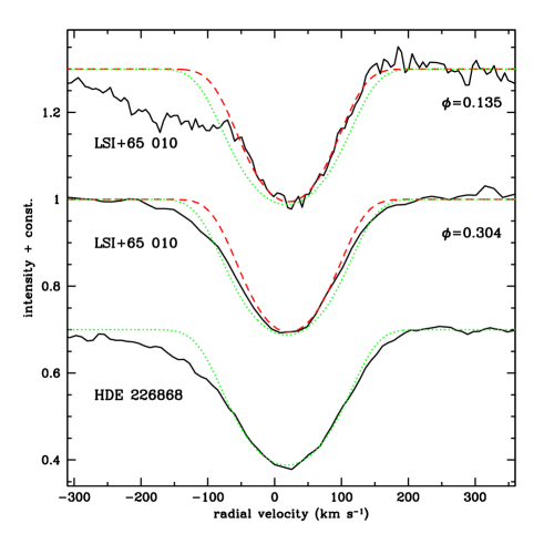
Figure 1: Observed line profiles of LSI$+$65 010 at two different orbital phases compared with theoretical lines profiles rotationally broadened to v sin(i)=96 km s^-1 (dashes) and 120 km s^-1 (dots), and with HDE 226868, the B-supergiant counterpart of Cyg X-1. Profiles are shifted by $\pm$0.03 on the vertical scale for clarity in the figure.

It is important to note that LSI+65 010’s profile at $\phi=$0.304 shown in Figure 1 substantially resembles HDE 226868’s line profile, as well as the theoretical profiles. Thus, the $\phi=$0.304 spectrum corresponds to a time when the B-supergiant is minimally perturbed and is probably the best profile for estimating v sin i . Adopting the value found by Reig et al. (1996) and the reported estimates of i $\sim$61$-$90^∘, v${}_{rot}\sim$96$-$109 km s^-1. The other stellar parameters derived for LSI+65 010 are M${}_{1}=$16$\pm$5 M_⊙, R${}_{1}=$37$\pm$15 R_⊙, and M${}_{2}=$1.7 M_⊙ for the neutron star (Reig et al. 1996).

Keeping M${}_{1}=$16 M_⊙, M${}_{2}=$1.7 M_⊙ and e=0 fixed, we performed a series of model calculations searching for variability on the P${}_{super}\sim$30.7 days, finding that P_super increases linearly with $\beta_{0}$ for $\beta_{0}$ in the range 0.57$-$0.63. P${}_{super}\sim$30.7 days was achieved with $\beta_{0}=$0.615. Fixing this value in Eq. (1) constrains R₁ to the range 36.2$-$41.1 R_⊙, for values of v_rot between 96$-$109 km s^-1. Figure 2 illustrates the characteristics of the “superorbital cycle” for two parameter sets (R₁,v_rot)=(40 R_⊙, 106 km s^-1) and (36.2 R_⊙, 96 km s^-1). A slow increase in the size of the tidal bulge over most of the cycle is followed by a more abrupt growth to an absolute maximum lasting $\sim$5 days. Oscillations on timescales of $\sim$hours also appear and, for the cases illustrated in Figure 2, they lie in the range 2-3 hours.

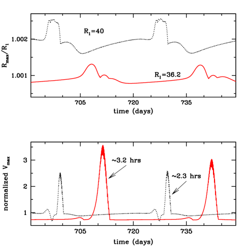
Figure 2: Radial extent of the tidal bulge, R_max (top), and maximum surface velocity, V_max, plotted as a function of time for circular orbit models with $\beta_{0}=$0.615. Results for two different stellar radii, R${}_{1}=$40 R_⊙ (dotted line; model C-1) and R${}_{1}=$36.2 R_⊙ (model C-2) are shown, illustrating the $\sim$31-day “superorbital” period that appears. Superposed oscillations on $\sim$hours timescales are indicated by the arrows, though they are barely visible on this figure.

In contrast to the circular orbit case, there are no “superorbital” periods on $\leq$100 day-timescales in eccentric orbit case, so the value of $\beta_{0}$ is unconstrained except for the limits on v_rot and R₁ given by Reig et al., which lead to the range $\beta_{0}\sim$0.40-0.90. An example of the tidal interactions predicted by the model for $\beta_{0}=$0.66 is shown in Figure 3. The data for one orbital cycle are plotted and the abscissa is given in units of orbital phase with periastron ($\phi=$0.0) and apastron indicated by the vertical tick marks. It is interesting to note that although the tidal bulge grows gradually as periastron is approached, it reaches maximum extent only after periastron passage due to the retarding action of the viscosity.

The short-timescale oscillations are most clearly seen in the bottom plot of Figure 3. Their frequency gradually decreases with time and corresponds to periodicities in the range $\sim$1.6-3.4 hours. The predicted amplitude is largest in the phase interval $\sim$0.15-0.40.

The idea of tidal oscillations in the tangential direction is somewhat less familiar than that of the radial oscillations. However, the “swashing” back and forth of the surface elements as they approach and pass the sub-stellar point is responsible for some of the strongest variability that is produced in photospheric line profiles. The tangential velocity perturbation, $\Delta$ V${}_{\Phi^{\prime}}$ for the e$=$0.16 case is illustrated in Figure 4 for different orbital phases, showing that the largest amplitudes occur near the primary tidal bulge, $\Phi^{\prime}\sim$360^∘. Note also that the perturbations are strongest after peristron passage, around orbital phase 0.20.

In Table 2 we list the observationally-derived parameters of LSI$+$65 010 as well as the parameters of the model calculations for the eccentric orbit and the two calculations for the circular orbit.

3.2 Viscosity and shear energy dissipation

The R${}_{1}=$40 R_⊙ models are highly unstable, which is easy to understand considering that this radius is very close to the Roche radius, requiring relatively large values of the viscosity to allow the computation to be performed. The oscillation amplitudes scale inversely with the viscosity, so larger amplitudes would be attained if we could use smaller $\nu$ values. However, as described by Moreno et al. (2005), when the oscillation amplitudes become too large, the individual surface elements for which the equations of motion are being solved become detached or begin to overlap, at which time the numerical computation is halted. To prevent this from happening, the value of $\nu$ may be increased. Our practice is to choose the smallest value of $\nu$ that allows the code to run over at least $\sim$5 orbital cycles in order to compute the line profiles after the initial transitory phase of the calculation. In the real star, the phenomena that we describe as “overlapping or detached surface elements” have no significance except that they suggest the possibility of large-scale relative motions that may be interpreted in terms of the more familiar term macro-turbulence. With this interpretation in mind, the value we use for $\nu$ in the calculations may be thought of as describing the conditions of the stellar surface at the limit where large-amplitude turbulent motions develop on small length scales.

The viscosity is related to the $\alpha$-parameter (Shakura & Sunyaev 1973) used in studies of accretion disks in Keplerian orbits through $\nu\sim(\alpha/\omega$)(kT/$\mu$m_H), where T is the temperature, $\mu$ is the mean molecular weight, and $\omega$ is a characteristic angular velocity. Associating $\omega$ with the relative motion of the external layer with respect to the rigidly-rotating inner region of our model, and assuming T=20,000 K, the values of $\nu$ we use in this paper all correspond to $\alpha<$0.01, well within the range expected for the outer layers of a supergiant star.

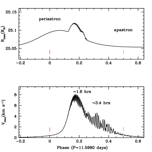
Figure 3: Radial extent of the tidal bulge, R_max, and maximum surface velocity, V_max, over one orbital cycle for the e=0.16 eccentric orbit. The abscissa is orbital phase. Periastron ($\phi=$0.0) and apastron are indicated. The short-timescale oscillations, best seen in the bottom panel, have periods $\sim$hours that gradually increase after periastron.

A direct consequence of the behavior of $\Delta V_{\Phi^{\prime}}$ and of including the viscosity in the calculation is that the surface layer sliding over the inner, rigidly-rotating body leads to shear energy dissipation, $\dot{E}$. Note that $\dot{E}$ is a potential source of additional energy that may be fed into the surface layers of the star and it has been suggested that $\dot{E}$ can contribute towards driving stellar winds or mass-ejections, or may play a role in the generation of magnetic fields (Koenigsberger et al. 2002; Moreno et al. 2005; Toledano et al. 2006). All these processes are generally associated with X-ray emission. Within this context, Figure 4 implies a concentration of surface activity on the hemisphere of M₁ that faces its companion. Hence, in addition to the effects produced by the accretion onto the neutron star and the ensuing X-ray emission, a strong degree of variability due to the activity on the B-star surface facing its companion is expected, particularly at periastron passage (if the orbit is eccentric).

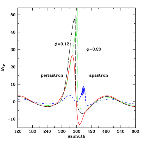
Figure 4: Azimuthal velocity perturbation of the surface layer as a function of angle for the eccentric orbit case for four different orbital phases, as indicated. Note that the largest azimuthal velocities occur near $\phi=$0.12, rather than at periastron passage. Large values of $\Delta$ V${}_{\Phi^{\prime}}$ lead to large energy dissipation rates.

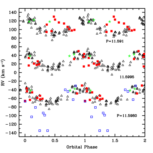
Figure 5: Radial velocity curves for three different periods: Crampton et al.’s (1985) 11.591 (top, shifted by +120 km s^-1), den Hartog et al.’s 11.5995 (middle, shifted by +60 km s^-1) and 11.5980 days (bottom). Data plotted are: Crampton et al. (1985) (open triangles), Reig et al. (open squares), our 1993 data (stars) and our 1995-2004 averages (filled squares) of at least 5 spectra per night.

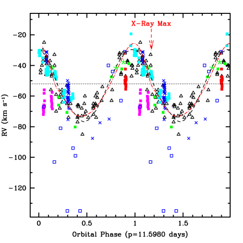
Figure 6: Radial velocity of Crampton et al. (open triangles), Reig et al. (open squares), and our measurements on individual spectra: REOSC echelle (crosses), UH coudé and MES-SPM (filled squares). The curves represent the RV that would be measured from of a M${}_{1}=$16 M_⊙ primary star tidally perturbed by a M${}_{2}=$1.7 M_⊙ companion in a $e=$0.16 (dot-dashes) or a circular (dashes) orbit. Phase 0.0 is maximum receding velocity for the circular orbit and periastron passage for the eccentric one. Time of X-ray maximum according to dem Hartog et al. ephemeris but with P=11.5980 days is indicated.

The two approximations used in our model calculations that must be noted are the artificial division of the star into an outer oscillating layer and an inner rigidly rotating body, and the fact that the calculation of the oscillations is performed only for the equatorial region of the star. The former limits the ability of the code to reproduce many of the oscillation frequencies that depend on the structure of the entire star, while the latter yields upper limits to the oscillation amplitudes since the strongest perturbations occur in the orbital plane. Finally, we note that the line-profile calculation does not currently include effects due to possible variations in the effective temperature over the stellar surface.

4 LSI+65 010: Results from the observational data

4.1 RV curve

The B-type optical counterpart of 2S0114+650, LSI+65 010=V662 Cas, was first identified by Margon & Bradt (1977) based on its variable H$\alpha$ emission and classified by Reig et al. (1996) and Liu & Hang (1999) as B1 Ia. Using measurements of photospheric absorption-line radial velocity (RV) variations from data obtained between 1978 and 1984, Crampton et al. (1985) concluded that the orbit of the B-supergiant was either circular, with P${}_{orb}^{circ}=$11.591$\pm$0.003 days or slightly eccentric (e$=$0.16), with P${}_{orb}^{ecc}=$11.588$\pm$0.003 days. Recently, den Hartog et al. (2006) found P${}_{orb}=$11.5995$\pm$0.0053 days from an analysis of RXTE-ASM and INTEGRAL data.

Figure 5 presents a plot (top) of the Crampton et al. (1985) data and our average data from Table 1 all folded in phase with the circular-orbit period and initial epoch. Our data in this figure are limited to points for which 5 or more individual spectra were obtained during the night. A significant phase shift between the modulation of the Crampton et al. (1985) data and the more recent data is evident. This phase shift is reduced if the data are folded with the den Hartog et al. P$=$ 11.5995 days (middle plot in Figure 5). An even better agreement between the two data sets is achieved with P$=$ 11.5980 days, which is well within the uncertainties given by den Hartog et al. The bottom plot of Figure 5 also includes the data published by Reig et al. (1996), obtained from RV measurements of He I 6678 Å. They follow in part the general trend of the other two data sets, but display significantly larger negative RV at phases $\sim$0.1-0.4 which correspond to orbital phases in which the secondary star is “in front” of the B-supergiant. This means that the photospheric absorption lines must have had a significantly more extended blue wing during these orbital phases, suggesting a difference between the hemisphere of the B-star that faces its companion and the opposite hemisphere. Considering the discussion of the previous section, we speculate that the difference between the two hemispheres may be associated with the tidal bulge and its oscillations.

In Figure 6 we now plot all the individual data measurements folded with P=11.5980 days and T${}_{0}=$43669.9 MJD. This value of T₀ is derived by taking the initial epoch given by Crampton et al. (1985) for their circular orbit solution and subtracting 40 cycles of 11.5980 days each. T₀ corresponds to the time of fastest receding radial velocity, which means that the hemisphere of the B-supergiant that faces its companion starts coming into view at $\phi=$0 and is occulted in our line-of-sight at $\phi>$0.5. The initial epoch T_ecc of the Crampton et al. (1985) eccentric orbit solution defines phase 0 as periastron passage. The different initial epochs are all listed in Table 2. We indicate with an arrow in Figure 6 the center of the broad X-ray maximum reported by den Hartog et al. According to their ephemeris, the X-ray “high” state is centered at $\phi\sim$0.12 for the circular orbit solution or $\phi\sim$0.07 if the orbit is eccentric. It is difficult to understand why X-ray maximum should be centered at these phases instead of around $\phi=$0.25 unless the orbit is eccentric, in which case X-ray maximum would occur very close to the phase for which our tidal model predicts maximum perturbation of the tidal bulge (see Figure 2).

The curves drawn in Figure 6 correspond to the two orbital solutions (e$=$0, e$=$0.16) but, compared to the large scatter of the data, are nearly indistinguishable. As we will show below, the dispersion of the RV data is intrinsic to the line profiles. Thus, the RV’s contain information additional to the orbital motion making the determination of the orbital solution very uncertain. It is interesting to note that the RV curves of other HMXRBs such as HD 153919/4U1700-37 (Hammerschlag-Henseberge et al. 2003) and HD77581/Vela X-1 (Barziv et al. 2001) also suffer from large intrinsic scatter, introducing significant uncertainties in the determination of the masses of their respective collapsed companions.

The individual RV measurements made on the MES-SPM data are plotted in Figure 7, showing that there is a systematic trend for cyclical variability with a characteristic timescale of $\sim$2.1 hours. The error bars correspond to the standard deviation of ISM line measurements, and are significantly smaller than the amplitude of the cyclic variation. The similarity between this variability timescale and P_flare is interesting, but we unfortunately do not have sufficient orbital phase coverage to establish when these cyclical variations are present and when they are not. There are two times in Figure 7 when they are absent, one of which ($\phi=$0.258), intriguingly, coincides with the conjunction corresponding to M₁ in back of its low-mass companion. If the optical $\sim$2-hour oscillations were intrinsic to the neutron star region, this would be the most favorable phase to observe them. The absence of oscillations at this phase is thus perplexing.

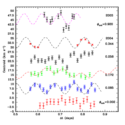
Figure 7: Centroids of individual spectra obtained in 2003 and 2004 with the MES-SPM spectrograph plotted as a function of time, with arbitrary initial times. Different nights are given a vertical shift for clarity. Error bars correspond to the uncertainties determined from the ISM-line measurements. The sine curves have frequency of 11.4 cycles day^-1.

4.2 Line profile variability

The large scatter in the RV curve of LSI+65 010 can be traced to line profile variability, as illustrated in Figure 8 where the He I 5875 Å line profiles are stacked in order of increasing phase. The shape of the observed profiles does not repeat with orbital phase, nor is there a clear pattern of variability over the orbital cycle. Some spectra display extraordinarily extended blue wings (e.g., the 1995 data) and some spectra have an extended “red” emission wing (e.g., orbital phases 0.002, 0.344, among others). In contrast, the line-profile variability that is predicted from the tidal oscillations is periodic with orbital phase, the strongest variations occuring in the phase interval 0.0$-$0.3. This is illustrated in Figure 9, where we plot the line profiles computed in the e$=$0.16 model. The perturbation on the line profile first appears at periastron passage on the blue wing and moves towards the red wing, becoming imperceptible by orbital phase $\sim$0.3. This pattern repeats over each orbital cycle. Hence, the observed behavior of He I 5875 Å indicates that its line profile is affected by processes in addition to the surface motions produced by the tidal forces.

A clue to the source of additional variability can be found by comparing the ratio of the perturbed and unperturbed theoretical profiles with the observational analogue. The left-hand panel of Figure 10 presents the theoretical residuals in the phase interval 0.96$-$1.43, showing the emission “bumps” and excess absorption features as they move accross the profile. These features are present only within the velocity range $\pm$100 km s^-1. The ratios of observed spectra were constructed using the 2001 Jan REOSC ($\phi=$0.304) spectrum in the denominator as a template, due to its apparently normal shape (see Figure 1). Before constructing the ratio, the template was shifted in velocity by amounts corresponding to the RV of the spectrum to be used in the numerator. Examples are shown in Figure 10 (right) and compared with theoretical residual spectra at the corresponding orbital phase. The observational residuals clearly extend over a broader velocity range and indicate the presence of actual superposed emission, not just the effects caused by ratio-ing line profiles affected by tidal oscillations. This is not surprising since we know that H$\alpha$ is in emission and that its line profile is variable (Margon & Bradt 1977; Koenigsberger et al. 2003). It is unfortunate, however, that our high resolution data do not include H$\alpha$ preventing us from searching for a connection between the H$\alpha$ emission and this deduced superposed emission. But a common source for both emissions is likely since the Gaussian full-width at half maximum intensity of the H$\alpha$ emission in the 2001 Oct spectrum is 280 km s^-1, which is similar to the width of some of the residual He I 5857 Å  profiles.

Whether the emission is produced in the vicinity of the collapsed companion or is associated with the B-supergiant can be answered with the radial velocity variations, as displayed in Figure 11. Although there is a trend for more negative RVs around $\phi=$0, just a few of the observations follow this trend, and the amplitude is only $\sim$70 km s^-1. This argues against the residual emission arising primarily in the vicinity of the collapsed object where large-amplitude RV variations associated with its orbital motion would be expected. Hence, we conclude that the wind close to the B-supergiant is the most likely source for the bulk of the superposed emission. The atmospheres of B-supergiants are, in general, very active and the He I 5875 Å line is reported to undergo large RV changes even in single stars (Kaufer et al. 2006; Morel et al. 2004), so the superposed emission in LSI+65 010 is just one more manifestation of the activity.

In summary, the observed line-profile variability in the He I 5875 Å line exceeds that which predicted from the tidal interaction model with input parameters as we have adopted for LSI$+$65 010. This is caused by superposed emission which we find to be associated primarily with the B-supergiant. The presence and variability of this emission indicates significant surface activity which, however, does not appear to correlate with orbital phase and may thus be similar to intrinsic variability that is observed for other B-type supergiants (Morel et al. 2004).

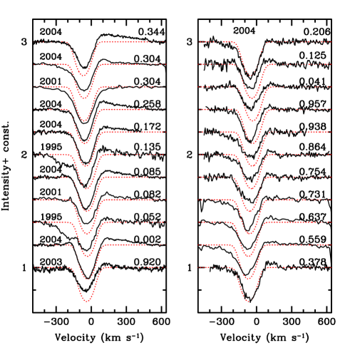
Figure 8: Montage of the He I 5875 Å  average (left) line profiles stacked in order of increasing orbital phase from bottom to top. The right-hand panel contains line profiles of nights for which only one or two spectra were acquired. Dotted profiles are the theoretical line profiles, rotationally broadened to v sin(i)=96 km s^-1, whose velocity shifts correspond to a Keplerian orbit of a 16 M_⊙ star with a 1.7 M_⊙ companion.

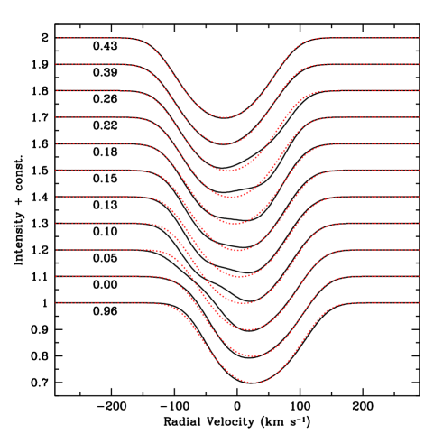
Figure 9: Theoretical model line-profiles stacked as a function of orbital phase for the tidally-perturbed 16 M_⊙, R${}_{1}=$25 R_⊙ star in the eccentric orbit. The dotted profiles correspond to the unperturbed line profiles. The strongest variability is observed between periastron passage ($\phi=$0.00) and $\phi\sim$0.30 and may be described in terms of a wave pattern that moves from the blue to the red wing.

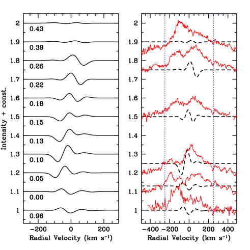
Figure 10: Left panel: Ratios of theoretical line profiles of the previous figure, illustrating the predicted differences between the perturbed and corresponding unperturbed photospheric absorption. Orbital phases are indicated. Right panel: Ratios of the observed profiles compared to the same theoretical variations (dashes) that are illustrated in the right-hand panel. The much broader velocity range in the observations (indicated by the vertical lines) implies the presence of residual emission, in addition to variability of the underlying photospheric absorption.

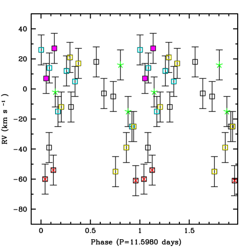
Figure 11: Centroid of the residual emission as a function of orbital phase. Stars represent the 1993 data; filled-in squares, the 1995 data; and open squares all other data except the 2004 Oct values which are indicated with crosses within open squares. A trend for more negative velocities around $\phi=$0 is present, although the small amplitude suggests an origin near the B-star rather than near the collapsed companion.

4.3 The 30.7 day “superorbital” period

If the “superorbital” period discovered by Farrell et al. is related to oscillations of the primary star, this period should appear in the optical data. Beskrovnaya (1988) reports polarization variations with a characteristic timescale of $\sim$month, supporting this possibility. Although this variability timescale is not apparent in the RV data, we do find indications of its presence in the strength of the residual emission. Figure 12 is a plot of the residual emission equivalent width measured by integrating over the entire emission feature, showing a possible modulation with P=30.79 days, which is within the $\pm$0.1 day uncertainty given by Farrell et al. The Farrell et al. T₀ corresponds to “minimum modulation of the light curve” which, according to their Fig. 3, occurs during the transition from minimum to maximum X-ray flux. Hence, the X-ray P_super “high” state is at phase $\phi_{super}\sim$0.25. This coincides with the general trend of the data in Figure 12.

The residual emission line profiles are illustrated in Figure 13 where they are stacked in order of increasing 30.79-day phase. There is a trend for broader and more symmetrical emission near phase 0 (bottom of the plot), with a narrower central peak developing thereafter. At other phases, two peaks are often observed, but the relative intensity of the two peaks can change from one night to the next.

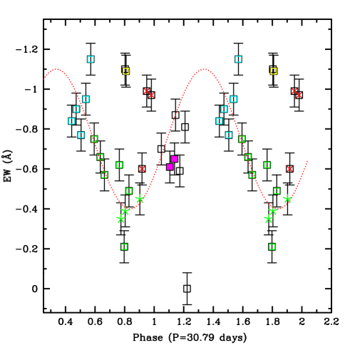
Figure 12: Equivalent width of the residual emission plotted as a function of the P${}_{super}=$30.79 day phase. A possible modulation is present, illustrated with a sine curve. Symbols are the same as in Figure 11. Here phase 0.0 corresponds to the time of minimum modulation in the X-ray light curve of Farrell et al., with X-ray “high” occuring near $\phi_{super}=$0.25.

Figure 13: He I 5875 Å residual emission stacked in order of increasing P${}_{super}=$30.79-day phase (from bottom to top), and with separations proportional to the $\phi_{super}$. As in Figure 12, zero phase corresponds to “minimum modulation” or the X-ray light curve (Farrell et al.). The arrows indicate our deduced approximate times of X-ray minimum ($\phi_{super}\sim$0.6-0.8) and X-ray maximum ($\phi_{super}\sim$0.1-0.3). Dots are used to differentiate between overlapping spectra on the plot.

Table 2: System and parameters for the eccentric (E) and two circular orbit (C1,C2) models.

Parameter	Empirical values	Model-E	Model-C1	Model-C2	Comments
Porb (days)	11.5995$\pm$0.0053	11.5980	11.5980	11.5980	den Hartog et al.
Psuper (days)	30.7	none	30.4	30.7	Farrell et al.
Pflare (hours)	$\sim$2.7	1.6$-$3.4	$\sim$2.3	$\sim$3.2	Hall et al.
$e$	0.0 or 0.16	0.16	0.00	0.00	Crampton et al.
Tecc (MJD)	44134.4	—	—	—	Crampton et al. eccentric orbit
Tcirc (MJD)	44133.8	—	—	—	Crampton et al. circular orbit
TX-orb (MJD)	51825.2	—	—	—	den Hartog et al. “X-ray maximum”
T0 (MJD)	43669.9	—	—	—	Tcirc-40 cycles; elongation
TX-super (MJD)	50108.2	—	—	—	Farrell et al. “minimum FX modulation”
M1 (M⊙)	16.0$\pm$5	16	16	16	Reig et al.
M2 (M⊙)	1.7	1.7	1.7	1.7	Reig et al.
R1 (R⊙)	37$\pm$15	25	40	36.2	Reig et al.
v sin i (km s-1)	96$\pm$20	100	96	96	Reig et al.
$i$ (deg)	61$-$90	90	65	90	Reig et al.
vrot (km s-1)	110	100	106	96
$\Omega_{per}$ (deg)	—	27	—	—	This paper
$\beta_{0}$	0.4-0.9	0.66	0.615	0.615	$\omega_{0}/\Omega_{per}$
$\nu$ (R${}_{\odot}^{2}$ day-1)	—	0.087	0.350	0.120	viscosity
$\delta$R/R1	—	0.0067	0.0050	0.0050	thickness of external layer

Figure 14: Schematic illustration of the scenario for the $\sim$2.7 hour X-ray periodicity, under the assumption that the oscillations near the tidal bulge are responsible for modulating the wind of the B-supergiant.

5 Conclusions

Tidal interactions in non-synchronously rotating binary systems produce strong perturbations on the external layers of the stars, particularly when the orbital separations are relatively small and the stellar radii are large. The binary system LSI$+$65 010=2S0114$+$650 is precisely such a system. The exploratory calculations performed for this paper are aimed at establishing the plausibility that the X-ray variability patterns of LSI+65 010$=$2S0114+650 may be attributable to these tidal interactions. We show that the oscillations on the surface of the B-supergiant that are predicted in our calculations have timescales that are consistent with the periodic timescales found in X-ray data. We propose that these oscillations may modulate the B-star’s wind, leading to a fluctuating accretion rate onto the neutron star, and hence, X-ray variability. Figure 14 is a cartoon depicting the scenario for oscillations with P$\sim$2-3 hours which are assumed to produce enhanced-density shells. This idea, originally proposed by Finley et al. (1992) was discarded when the optical component of 2S0114$+$650 was found to be a B-supergiant instead of a $\beta$ Cep-type star, since such short timescale pulsations are not predicted for single supergiant stars. We rescue Finley et al.’s hypothesis by proposing that the presence of a companion can lead to the appearance of such short periods.

The precise mechanisms by which the oscillations may translate into a structured stellar wind are not clear, but we speculate that an answer may lie in the combination of the radial pulsation components and the shear energy dissipation due to the tangential motions of the outer stellar layers sliding over the more slowly rotating inner layers. These two combined sources (the radial pulsation component and the shear energy dissipation), when added to the radiation field that normally drives the stellar wind, might cause the inhomogeneities to appear on the same timescale as that of the largest amplitude oscillations. In order to establish a connection between the tidal oscillations and the modulation of mass-ejection in LSI$+$65 010, it is necessary to analyze spectral lines that are less susceptible to contamination from emission, together with observations of H$\alpha$. It is important to note that such observations have been successfully performed in other stars (Fullerton, Gies & Bolton 1996; Prinja et al. 2004; Kaufer et al. 2006) showing a link between photospheric activity and perturbations in the dense inner regions of stellar winds.

It is interesting to note that the largest oscillation amplitudes induced by the tidal forces occur near the primary tidal bulge. Hence, the periodic modulation of the stellar wind may only be present in a small solid angle oriented in the general direction of the neutron star. The localized nature of the oscillations would explain the lack of a clear $\sim$2.7 hr periodicity in the He I 5875 Å  data, since the irregular variations that are present over the whole B-star surface most likely drown out the small-scale periodic effects. Thus, an interesting conclusion is that the X-ray emission is a much finer diagnostic of the local wind structure than the optical line profiles, the latter reflecting the integral of the absorption/emission over the stellar disk.

The tidal interaction model predicts a large difference between the pulsation energy dissipation rates, $\dot{E}$, near periastron and apastron for an eccentric orbit. This implies a significant variation in surface activity as a function of orbital phase, assuming that the surface activity is associated with $\dot{E}$. X-ray variability on the orbital timescale is indeed present, but the line profiles in our optical data do not display strong changes between periastron and apastron phases, weakening the case for an eccentric orbit. In a circular orbit, $\dot{E}$ remains constant over orbital phase and thus no modulation of the stellar wind with P_orb is expected. If the orbit of LSI$+$65 010 is circular, the observed X-ray variability is likely due to eclipse effects, rather than to differences in the accretion rates onto the companion. A circular orbit would also be consistent with the existence of a “superorbital” period.

Our final consideration concerns the possibility that part of the X-ray emission may actually originate in the B-supergiant. In particular, the tangential component of the perturbation produces a differentially rotating structure in the surface layers that one might speculate could lead to magnetic field generation. Admittedly, the timescales over which a particular region of the star develops this structure may be too short for magnetic field amplification mechanisms for massive stars, such as proposed by Spruit (2002), to operate. However, it would be interesting to explore the mechanisms that could convert tidal energy into magnetic field energy, as has been done for low-mass stars (for example, Zaqarashvili et al. 2002). Furthermore, observational evidence for surface magnetic field structures in OB stars now exists (Henrichs, Neiner, Geers 2003), so it would be interesting also to explore the effects of the tidal oscillations on assumed pre-existing magnetic field structures and determine the X-ray emitting characteristics due to these perturbations.

- (1) Barziv, O., Kaper, L., Van Kerkwijk, M.H., Telting, J.H., Van Paradijs, J. 2001, A&A 377, 925.
- (2) Beskrovnaya, N.G. 1988, Sov. Astron. Lett. 14, 314.
- (3) Corbet, R. H. D., Finley, J.P., Peele, A.G. 1999, ApJ 511, 876.
- (4) Crampton, D., Hutchings, J.B., Cowley, A.P. 1985, ApJ 299, 834.
- (5) Diego, F. & Echeverria, J. 1994, Reporte Técnico, Instituto de Astronomía, UNAM.
- (6) Dower, R., Kelley, R., Margon, B., Bradt,H. 1977, IAUC 3144.
- (7) Farrell, S.A., Sood, R.K., O’Neill, P.M. 2006, MNRAS, 367, 1457.
- (8) Finley, J.P., Belloni, T., Cassinelli, J.P. 1992, ApJ 262, L25
- (9) Finley, J.P., Taylor, M., Belloni, T. 1994, ApJ 429, 356.
- (10) Hammerschlag-Henseberge, G., van Kerkwijk, M. H. and Kaper, L. 2005, A&A, in Press, arXiv: astro-ph/0307119 (2003).
- (11) den Hartog, P.R., Hermsen, W., Kuiper, L., Vink, J., in’t Zand, J.J.M and Collmar, W. 2006, A&A, in Press.
- (12) Hall, T.A., Finley, J.P., Corbet, R.H.D., Thomas, R.C. 2000, A&A 536, 450.
- (13) Henrichs, H.F., Neiner, C., Geers, V.C. 2003, in Proceedings IAU Symposium 212, van der Hucht, Herrero & Esteban (eds.), ASP Conference Series, p. 202.
- (14) Kaufer, A., Stahl, O., Prinja, R.K., Witherick, D. 2006, A&A 447, 325.
- (15) Koenigsberger, G., Swank, J.H., Szymkowiak, A.E., White, N.E. 1983, ApJ 268, 782
- (16) Koenigsberger, G., Canalizo, G., Arrieta, A., Richer, M., Georgiev, L. 2003, RMAA, 39, 1.
- (17) Kumar, P., Ao, C.O., Quataert, E.J. 1995, ApJ, 449, 294.
- (18) Li, X.-D., van den Heuvel, E.P.J. 1999, ApJ 513, L45
- (19) Margon, B. & Bradt, H.V. 1977, IAU Circ. No. 3144.
- (20) Morel, T., Marchenko, S.V., Pati, A.K., Kuppuswamy, K., Carini, M.T., Wood, E., Zimmerman, R. 2004, MNRAS, 351, 552
- (21) Moreno, E. & Koenigsberger, G. 1999, RMA&A, 35, 157
- (22) Moreno, E., Koenigsberger, G. & Toledano, O. 2005, A&A, 437, 641.
- (23) Reig, P., Chakrabarty, D., Coe, M.J., Fabregat, J., Negueruela, I., Prince, T.A., Roche, P., Steele, I.A. 1996, AA 311, 879.
- (24) Mukherjee, U. & Paul, B. 2006, J. Astrophys. Astr., in press, (arXiv:astro-ph/0602558 v1.)
- (25) Prinja, R.K., Rivinius, Th., Stahl, O., Kaufer, A., Foing, B.H., Cami, J., Orlando, S. 2004, A&A 418, 727.
- (26) Richer, M. 2003, “The efficiency, stability, and lamp identifications for the MES-SPM spectrometer”, Technical Report, OAN/SPM.
- (27) Savonije, G.J., Papaloizou, J.C.B., & Alberts, F. 1995, MNRAS 277, 471
- (28) Shakura, N.I. & Sunyaev, R.A. 1973, A&A, 24, 337
- (29) Spruit, H.C. 2002, A&A 381, 923.
- (30) Toledano, O., Moreno, E., Koenigsberger, G., Detmers, R., Langer, N. 2006, A&A,
- (31) Yamauchi, S., Asaoka I., Kawada M., Koyama K. and Tawara Y., 1990, PASJ 42, L53
- (32) Zahn, J.-P. 1977, A&A 57, 383
- (33) Zaqarashvili, T., Javakhishvili, Belvedere, G. 2002, ApJ579, 810.