Abstract

Model selection aims to determine which theoretical models are most plausible given some data, without necessarily asking about the preferred values of the model parameters. A common model selection question is to ask when new data require introduction of an additional parameter, describing a newly-discovered physical effect. We review several model selection statistics, and then focus on use of the Bayesian evidence, which implements the usual Bayesian analysis framework at the level of models rather than parameters. We describe our CosmoNest code, which is the first computationally-efficient implementation of Bayesian model selection in a cosmological context. We apply it to recent WMAP satellite data, examining the need for a perturbation spectral index differing from the scale-invariant (Harrison–Zel’dovich) case.

1 Introduction

Cosmologists are becoming very good at determining the parameters of the Universe. Within the last few years observational results, exemplified by the microwave background anisotropy measurements by the Wilkinson Microwave Anisotropy Probe (WMAP), have introduced precision into cosmological modelling. Considerable sophistication is now required both in deriving theoretical predictions from models and in carrying out data analysis procedures able to squeeze the best from the data.

Within a cosmological model, the parameters indicate the importance of different effects. For instance, they describe the relative amounts of different types of material in the Universe, the geometry and expansion rate of the Universe, and the properties of the initial irregularities in the Universe which led to the formation of structure. Such parameters are not predicted by fundamental theories, but rather must be fit from data in order to decide which combination, if any, is capable of describing our Universe. A variety of cosmological data are currently well fit by a model of the Universe that is homogeneous, isotropic and spatially flat, contains cold dark matter in greater proportions than ordinary baryonic matter, and in which tiny initial perturbations evolved under Einstein’s theory of General Relativity into the structures of today. Current data constrain the parameters of this model rather well, many at the 10% level or better.

However, the presence of good data leads to a different problem, one of knowing when to stop fitting. Two different and competing models of the Universe may explain the data equally well, so how do we choose between them? The solution is one proposed by William of Occam, that the simpler model should be preferred. This is known as Occam’s razor. So a complicated model that explains the data slightly better than a simple one should be penalized for the extra parameters it introduces, because the extra parameters bring with them a lack of predictability. On the other hand, if a model is too simple, and cannot fit certain data well, then it can be discarded. This is a rather common type of statistical problem, both in cosmology and in other fields of astrophysics: each available parameter within a model describes some piece of physics that might be relevant to our Universe, but until measurements are made we don’t know which.

Cosmological model selection refers to comparing different model descriptions of the data. It doesn’t care particularly about the actual values of parameters, but rather aims to determine which set of parameters gives the preferred fit to observational data.

2 Why model select?

Model selection is an extremely widespread challenge throughout science; how do you fit to data when you are unsure about the set of parameters that you should be deploying. You cannot just include every parameter you can think of in a fit to data, because inclusion of extra unnecessary parameters worsens the determination of those that are essential, so that very soon you can end up learning nothing about anything. Moreover, you can’t just use goodness of fit to the data, because typically inclusion of a new parameter will improve the goodness of fit even if that parameter has absolutely no actual relevance to the Universe. Typical attempts to avoid these problems involve ad hoc criteria such as ‘chi-squared per degrees of freedom’ arguments or the ‘likelihood ratio test’, in which arbitrary thresholds have to be invoked to decide which way the verdict is supposed to go. Model selection aims to put this practice on a firmer footing.

Model selection problems are ones in which the parameter set necessary to describe a given dataset is unknown, the question typically being whether new data justifies inclusion of a new physical parameter. Many of the most pressing questions in astrophysics are of this form. Cosmological examples would include whether the spatial curvature is non-zero, whether the dark energy density evolves, and whether the initial perturbation spectrum has an amplitude which varies with length scale.

3 Model selection statistics

The generic purpose of a model selection statistic is to set up a tension between the predictiveness of a model (for instance indicated by the number of free parameters) and its ability to fit observational data. Oversimplistic models offering a poor fit should of course be thrown out, but so should more complex models which offer poor predictive power.

There are two main types of model selection statistic that have been used in the literature so far. Information criteria look at the best-fitting parameter values and attach a penalty for the number of parameters; they are essentially a technical formulation of ‘chi-squared per degrees of freedom’ arguments. By contrast, the Bayesian evidence applies the same type of likelihood analysis familiar from parameter estimation, but at the level of models rather than parameters. It depends on goodness of fit across the entire model parameter space.

Here we discuss three possible statistics. In each case, the statistic is a single number that is a property of the model, and having computed it the models can be placed in a rank-ordered list.

Akaike Information Criterion (AIC):

This was derived by Hirotugu Akaike in 1974, and takes the form

$${\rm AIC}=-2\ln{\cal L}_{\rm max}+2k\,,$$ (1)

where ${\cal L}$ is the likelihood ($-2\ln{\cal L}$ is often called $\chi^{2}$ though it generalizes it to non-gaussian distributions) and $k$ is the number of parameters in the model. The subscript ‘max’ indicates that one should find the parameter values yielding the highest possible likelihood within the model. It is obvious that this second term acts as a kind of ‘Occam factor’; initially as parameters are added the fit to data improves rapidly until a reasonable fit is achieved, but further parameters then add little and the penalty term $2k$ takes over. The generic shape of the AIC as a function of number of parameters is therefore a rapid fall, a minimum, and then a rise. The preferred model sits at the minimum.

The AIC was derived from information-theoretic considerations, specifically an approximate minimization of the Kullback–Leibler information entropy which measures the distance between two probability distributions.

Bayesian Information Criterion (BIC):

This was derived by Gideon Schwarz in 1978, and strongly resembles the AIC. It is given by

$${\rm BIC}=-2\ln{\cal L}_{\rm max}+k\ln N\,,$$ (2)

where $N$ is the number of datapoints. Since a typical dataset will have $\ln N>2$, the BIC imposes a stricter penalty against extra parameters than the AIC.

It was derived as an approximation to the Bayesian evidence, to be discussed next, but the assumptions required are very restrictive and unlikely to hold in practice, rendering the approximation quite crude.

Bayesian evidence:

The Bayesian evidence looks rather different, being defined as

$$E=\int{\cal L}(\theta){\rm Pr}(\theta)d\theta\,.$$ (3)

Here $\theta$ is the vector of parameters of the model, and ${\rm Pr}(\theta)$ is the prior distribution of those parameters before the data were obtained. The prior is an essential part of the definition of a model, upon which the evidence will ultimately depend, and might for instance be a set of ranges within which parameters are assumed to be uniformly distributed.

The evidence of a model is thus the average likelihood of the model in the prior. Unlike the statistics above, it does not focus on the best-fitting parameters of the model, but rather asks “of all the parameter values you thought were viable before the data came along, how well on average did they fit the data?”. Literally, it is the likelihood of the model given the data. Given Bayes’ theorem

$$P(M|D)=\frac{P(D|M)P(M)}{P(D)}\,.$$ (4)

(here M is the model, D is the data, and the vertical bar is read as ‘given’), the evidence $E\equiv P(D|M)$ updates the prior model probability $P(M)$ to the posterior model probability $P(M|D)$, i.e. the probability of the model given the data.

The evidence rewards predictability of models, provided they give a good fit to the data, and hence gives an axiomatic realization of Occam’s razor. A model with little parameter freedom is likely to fit data over much of its parameter space, whereas a model which could match pretty much any data that might have cropped up will give a better fit to the actual data but only in a small region of its larger parameter space, pulling the average likelihood down.

The evidence is also known as the marginalized likelihood or, more accurately, the model likelihood. The ratio of evidences for two models is known as the Bayes factor.

Of these statistics, we would advocate using, wherever possible, the Bayesian evidence which is a full implementation of Bayesian inference and can be directly interpreted in terms of model probabilities. It is computationally challenging to compute, being a highly-peaked multi-dimensional integral, but recent algorithm development has made it feasible in cosmological contexts. We discuss it further in the next section.

If the Bayesian evidence cannot be computed, the BIC can be deployed as a substitute. It is much simpler to compute as one need only find the point of maximum likelihood for each model. However interpreting it can be difficult. Its main usefulness is as an approximation to the evidence, but this holds only for gaussian likelihoods and provided the datapoints are independent and identically distributed. The latter condition holds poorly for the current global cosmological dataset, though it can potentially be improved by binning of the data hence decreasing the $N$ in the penalty term.

The AIC has been widely used outside astrophysics, but is of debatable utility. Sometime after it was first derived, it was shown to be ‘dimensionally inconsistent’, a statistical term meaning that it is not guaranteed to give the right result even in the limit of infinite unbiased data. It may however be useful for checking the robustness of conclusions drawn using the BIC. The evidence and BIC are dimensionally consistent.

4 Computing and interpreting the evidence

Computing the evidence in realistic problems is challenging, particularly in cosmology where evaluating theoretical predictions at just a single parameter point requires several seconds of CPU time with state-of-the-art codes such as cmbfast or camb. Markov chain Monte Carlo (MCMC) methods are now commonplace in cosmological parameter estimation, and efficiently trace the posterior probability distribution of the parameters of a model in the vicinity of the best-fit region. However a different sampling strategy is needed to evaluate the evidence. It can receive a large contribution from the tails of the posterior distribution of the parameters, because even though the likelihoods there are small, this region occupies a large volume of the prior probability space. Therefore the sampling strategy must effectively sample the entire prior volume to evaluate the integral (Eqn 3) accurately. Until recently, the best available strategy for evidence calculation, known as thermodynamic integration or simulated annealing, required around $10^{7}$ likelihood evaluations for an accurate answer for a five-parameter cosmological model, placing the problem at the limit of current supercomputer power.

Fortunately, a powerful new algorithm for evidence evaluation, known as nested sampling, was recently invented by John Skilling (2004). At Sussex we have implemented this algorithm for cosmology in a code named CosmoNest, which we recently made publically available. It has proven to be one to two orders of magnitude more efficient than thermodynamic integration, meaning that evidence calculations can now be run on a small computing cluster.

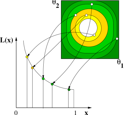
Figure 1: A schematic of the nested sampling algorithm. The two-dimensional parameter space is shown at the top right. The points within it are considered to represent contours of constant likelihood, which sit within each other like layers of an onion (there is however no need for them to be simply connected). The volume corresponding to each thin shell of likelihood is computed by the algorithm, allowing the integral for the evidence to be accumulated as shown in the graph.

To set up the algorithm, the evidence integral is first recast as a one-dimensional integral in terms of the prior mass $X$, where $dX=\mathrm{Pr}(\theta)\,d\theta$ with $X$ running from 0 to 1. [A mental image to accompany this is to consider the prior parameter space as a cube, and to smash it with a large hammer. The fragments are then arranged in a line in order of increasing likelihood.] The algorithm samples the prior a large number of times, assigning a ‘prior mass’ to each sample. The samples are ordered by likelihood, and the integration follows as the sum of the sequence,

$$E=\int L(X)dX=\sum_{j=1}^{m}E_{j}\,,\quad E_{j}=\frac{L_{j}}{2}(X_{j-1}-X_{j+1})\,.$$ (5)

This is shown in Figure 1.

In order to compute the integral accurately the prior mass is logarithmically sampled. We start by randomly placing a set of $N$ points within the prior parameter space, where in a typical cosmological application $N\simeq 300$. We then iteratively discard the lowest likelihood point $L_{j}$, replacing it with a new point uniformly sampled from the remaining prior mass (i.e. with likelihood greater than $L_{j}$). Each time a point is discarded the prior mass remaining, $X_{j}$, shrinks by a factor that is known probabilistically, and the evidence is incremented accordingly. In this way the algorithm works its way towards the higher likelihood regions. The process is illustrated in Figure 2. Additional details of the algorithm are in Mukherjee, Parkinson & Liddle (2006a). The algorithm is simple, works accurately even in high dimensions, and should be generally applicable in a number of areas even outside of astrophysics.

Although the evidence gives a rank-ordered list of models, it is still necessary to decide how big a difference in evidence is needed to be significant. If the prior probabilities of the models are assumed equal, the difference in log(evidence) can be directly interpreted as the relative probabilities of the models after the data. Even if people disagree on the relative prior probabilities, they will all agree on the direction in which the data, represented by the evidence, has shifted the balance. The usual interpretational scale employed is due to Sir Harold Jeffreys (from his classic 1961 book ‘Theory of Probability’), which, given a difference $\Delta\ln E$ between the evidences $E$ of two models, states that

$\Delta\ln E<1$	Not worth more than a bare mention.
$1<\Delta\ln E<2.5$	Significant.
$2.5<\Delta\ln E<5$	Strong to very strong.
$5<\Delta\ln E$	Decisive.

In practice we find the divisions at 2.5 (corresponding to posterior odds of about 13:1) and 5 (corresponding to posterior odds of about 150:1) the most useful.

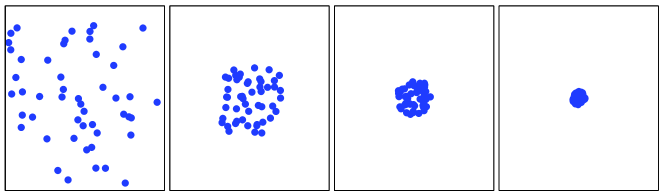
Figure 2: A sequence of snapshots of a toy-model evidence calculation, using a two-dimensional gaussian likelihood. As the computation progresses the cluster of points, initially distributed throughout the parameter space, drifts towards the region of high likelihood at the centre.

When should model selection be deployed? If the data indicates something strongly enough, it doesn’t really matter how the statistical analysis is done. The main zone of interest is where a new parameter is ‘detected’ at between two and four ‘sigmas’ via parameter estimation techniques. These overestimate the significance of a detection because they ignore model dimensionality, and there is a well-known (in the statistics literature anyway) phenomenon called Lindley’s paradox, whereby model selection considerations can overturn an analysis based on a ‘number of sigmas’ argument. A nice discussion of Lindley’s paradox is given in Trotta (2005).

One of the bugbears of Bayesian methods is the requirement to specify priors explicitly, with the evidence depending on the choice of priors. If the data have low informative content (technically defined via the ratio of prior and posterior parameter volumes), this can be a serious issue, but it becomes less so if the data are constraining so that the posterior is well localized within any conceivable prior. In that case the evidence becomes proportional to the prior volume, and quite a substantial change in volume is needed to move models significantly around the Jeffreys scale.

5 Applications of model selection

There are several areas of application of model selection techniques, the main two being as follows:

Application to data:

With real data, one can assess the viability of different models under consideration. In this case one simply computes the evidence for each model of interest and ranks them.

Model selection forecasting:

This application aims to compare the power of different experiments before they are carried out. Many proposed experiments seek to answer model selection questions, but their capabilities are often quantified using parameter estimation projections, such as Fisher matrix forecasting. For instance, a dark energy experiment may be advertized as able to measure the equation of state parameter $w$ with an uncertainty of $\pm 0.05$, the aim being to detect deviations of $w$ from $-1$, which characterizes the cosmological constant or vacuum zero-point energy. One can instead forecast experiments’ ability to carry out model selection tests. In this case data must be simulated for a range of different assumed models, in order to investigate where in the available parameter space a given experiment can make a strong or decisive model comparison between a dynamical dark energy model and the cosmological constant. This gives a powerful tool for comparing the statistical power of competing experiments. It should also be possible to extend this concept to survey optimization, whereby one tunes survey parameters to optimize the ability to carry out model selection tests, but it is less clear that this will be fruitful.

We have extensively discussed the philosophy of model selection forecasting, with specific application to dark energy experiments, in Mukherjee et al. (2006b). In Pahud et al. (2006) we applied these ideas to determination of the nature of the primordial power spectrum of density perturbations, focussing on the ability of the Planck Satellite mission to perform model selection of this type. In this article we will focus on applications to real data.

5.1 A toy model

To help understand what is going on, we can carry out a simple toy model investigation into the spatial curvature of the Universe. According to the three-year data from WMAP (henceforth WMAP3), the total density, in units of the critical density, is $\Omega=1.003\pm 0.015$ (where we took the liberty of symmetrizing the uncertainty and where the Hubble Key project determination of the Hubble parameter is also used). Given this, how likely is it that the Universe is flat? For simplicity we’ll assume a gaussian likelihood corresponding to this measurement, and ignore dependence on other parameters, so we have

$${\cal L}={\cal L}_{0}\exp\left[-\frac{\left(\Omega-1.003\right)^{2}}{2\times 0.015^{2}}\right]$$ (6)

We also have to choose a prior range for $\Omega$; let’s say $0.1<\Omega<2$ representing some plausible range people might have considered long before precision data emerged. Now the calculation, remembering that the evidence is just the average likelihood over the prior.

Flat model:

We just have to evaluate the likelihood at $\Omega=1$. It is $E({\rm flat})=0.98{\cal L}_{0}$.

Curved model:

Now we have to integrate the likelihood over the prior, being sure to normalize the prior properly. This gives $E({\rm curved})=0.02{\cal L}_{0}$.

The conclusion is that, under these assumptions, the flat model is preferred at odds of approximately 50:1.

That example was pretty boring, since $\Omega=1$ lies almost in the middle of the measured range. But suppose the result had been $\Omega=1.045\pm 0.015$, a putative three-sigma detection of spatial curvature. The evidence for the curved model is unchanged (it doesn’t care what the measured value is provided it is well within the prior) while that of the flat model shrinks. Nevertheless, the end result is an odds ratio of only 2:1 in favour of the curved model. In this case, three-sigma is nowhere near enough to convincingly indicate that space is curved. Physically, the evidence is allowing for it being a priori very unlikely that $\Omega$ could be so close to one as to give such a low-confidence ‘detection’, yet still not be equal to one. Put another way, the $\Delta\ln E$ would be 0.7 which according to Jeffreys is hardly worth mentioning.

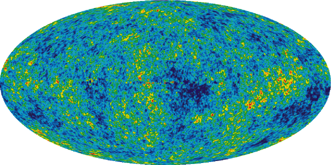
Figure 3: A composite map of the cosmic microwave background (CMB) as measured by three years of WMAP observations. The colour scale indicates the CMB temperature and the whole sky is shown in Hammer–Aitoff projection in galactic coordinates. Measurements at different frequencies have used to model out non-CMB contributions, particularly galactic emission. [Image courtesy NASA/WMAP Science Team.]

5.2 Real cosmology

Now we turn to a real cosmological example. The new three-year data from WMAP (see Figures 3 and 4) is for the most part uncontroversial from a model selection point of view, with parameters either being definitely required or clearly unnecessary. The exception is the scale dependence of primordial density perturbations, defined by the spectral index $n_{{\rm S}}$. These perturbations are usually considered to have been generated by inflation, a period of rapid acceleration in the early Universe. As well as solving some of the problems with the traditional hot big bang model, inflation also generically predicts the kind of observations that we now see. The many models of inflation predict a wide range of possible values for $n_{{\rm S}}$, which one should then try and fit from the data.

Figure 4: Upper panel: the CMB temperature power spectrum measurements from WMAP3 (black dots, with error bars) shown against a model power spectrum that provides a good fit (red curve). Bottom panel: the CMB temperature–polarization cross-correlation measurements from WMAP (blue dots with error bars) shown against the predictions of the same model as above (green curve). [Image courtesy NASA/WMAP Science Team.]

However, a decade before inflation was invented, Harrison and Zel’dovich independently proposed that $n_{{\rm S}}$ should be precisely one, corresponding to perturbations whose amplitude is independent of scale. At least until this year’s publication of the three-year WMAP data, the Harrison–Zel’dovich spectrum always gave a good fit to existing data. From a model selection perspective it benefits from having one parameter less than a model where $n_{{\rm S}}$ varies, and indeed we showed in a paper last year predating WMAP3 that the Harrison–Zel’dovich model had the highest evidence, though other models including varying $n_{{\rm S}}$ were not strongly excluded.

WMAP3 gave, for the first time, indications that $n_{{\rm S}}$ might be less than one, with their main paper quoting the results (from WMAP3 data alone) $n_{{\rm S}}=0.951^{+0.015}_{-0.019}$, which thus appears to be over 3-sigma away from unity. A similar result is found when WMAP data is combined with other independent datasets, such as the power spectrum of the large-scale distribution of galaxies and the redshift–luminosity relation of distant type Ia supernovae. So far, parameter estimation analyses performed on available data taken together seem to indicate that $n_{{\rm S}}\neq 1$ at about 3 to 4-sigma.

This significance level is exactly where Lindley’s paradox is at its strongest, making the use of model selection techniques imperative, as acknowledged in the WMAP3 papers. We have carried out such an analysis. We chose a prior on $n_{{\rm S}}$ uniform between 0.8 between 1.2; most inflationary models give $n_{{\rm S}}$ in this range and this is what was believed to be the possible range for it before the data came along. Evidences were computed using CosmoNest, with the calculations taking a few days on a multi-processor cluster.

According to our model selection analysis, the evidence for the $n_{{\rm S}}$ varying model is significant, but not strong or decisive. WMAP3 data on its own gives a Bayes factor of only $0.34\pm 0.26$, indicating that this data alone is unable to distinguish the two models. When WMAP3 data are used together with external data sets we estimate a $\Delta\ln E$ of $1.99\pm 0.26$, corresponding to an odds ratio of 8 to 1 in favour of the $n_{{\rm S}}$ varying model. Adding the external datasets improves the constraining power on $n_{{\rm S}}$, as they significantly extend the scales over which the primordial power spectrum affects the data. Nevertheless, the support for varying $n_{{\rm S}}$ is clearly tentative rather than compelling.

There is additional reason for some caution at present because there may be residual systematics in the data that could affect our conclusions regarding $n_{{\rm S}}$; the evidence calculation concerns statistical uncertainties only. For example, the effect of varying $n_{{\rm S}}$ in determining the power spectra shown in Figure 4 is somewhat degenerate with the signature of the relatively recent reionization of the Universe, which is mainly inferred from polarization data which is difficult to handle. There are also uncertainties associated with the modelling of the instrument beam profiles, and in whether one should attempt to model out a possible contribution to the CMB anisotropies from the Sunyaev–Zel’dovich effect. The situation will be improved with higher signal-to-noise data from additional years of WMAP observations and future experiments.

6 Conclusion

Many of the most interesting cosmological questions are ones of model selection, not parameter estimation. With the growing precision of cosmological data, it is imperative to deploy proper model selection techniques to extract the best robust conclusions from data.

Application to the post-WMAP3 cosmological data compilation continues to indicate that the data can be well fit by quite minimal cosmological models. Five fundamental parameters are definitely required, and WMAP3 has provided suggestive indications that a sixth, the density perturbation spectral index, needs to be added to the set. According to the Bayesian evidence, however, the case for inclusion of the spectral index has yet to become compelling.

As the data improve in sensitivity we expect new model selection based questions to be both raised and answered in the next decade. These may be about the nature of dark energy, the model for reionization, the nature of inflation, the case for primordial gravitational waves, or the nature of cosmic topology. Model selection, of course, will have further applications in astrophysics and beyond.

Bibliography

Jeffreys H 1961, Theory of Probability, 3rd edition [OUP, Oxford].

Liddle A R 2004, MNRAS 351 L49-L53

Mukherjee P, Parkinson D, Liddle A R 2006a, ApJ 638 L51-L54

Mukherjee P, Parkinson D, Corasaniti P S, Liddle A R, Kunz M 2006b, MNRAS 369, 1725–1734

Parkinson D, Mukherjee P, Liddle A R 2006, Phys. Rev. D 73, 123523

Pahud C, Liddle A R, Mukherjee P, Parkinson D 2006, Phys. Rev. D 73, 123524

Skilling J 2004, in Bayesian Inference and Maximum Entropy Methods in Science and Engineering ed. R. Fischer et al. [Amer. Inst. Phys., conf. proc.,] 735 395

Trotta R 2005, astro-ph/0504022