Is the dark matter halo of the Milky Way flattened?

We performed an extended analysis of the parameter space for the interaction of the Magellanic System with the Milky Way (MW). The varied parameters cover the phase space parameters, the masses, the structure, and the orientation of both Magellanic Clouds, as well as the flattening of the dark matter halo of the MW. The analysis was done by a specially adopted optimization code searching for the best match between numerical models and the detailed H I map of the Magellanic System by Brüns et al. (Bruens05 (2005)). The applied search algorithm is a genetic algorithm combined with a code based on the fast, but approximative restricted N–body method. By this, we were able to analyze more than $\mathrm{10^{6}}$ models, which makes this study one of the most extended ones for the Magellanic System. Here we focus on the flattening $q$ of the axially symmetric MW dark matter halo potential, that is studied within the range $0.74\leq q\leq 1.20$. We show that creation of a trailing tail (Magellanic Stream) and a leading stream (Leading Arm) is quite a common feature of the Magellanic System–MW interaction, and such structures were modeled across the entire range of halo flattening values. However, important differences exist between the models, concerning density distribution and kinematics of H I, and also the dynamical evolution of the Magellanic System. Detailed analysis of the overall agreement between modeled and observed distribution of neutral hydrogen shows that the models assuming an oblate ($q<1.0$) dark matter halo of the Galaxy allow for better satisfaction of H I observations than models with other halo configurations.

1 Introduction

The idea of dark matter (DM) was introduced by Zwicky (Zwicky33 (1933)). His dynamical measurements of the mass–to–light ratio of the Coma cluster gave larger values than those known from luminous parts of nearby spirals. That discrepancy was explained by the presence of DM. Ostriker et al. (Ostriker74 (1974)) proposed that DM is concentrated in a form of extended galactic halos. Analysis of rotation curves of spiral galaxies (Bosma Bosma81 (1981); Rubin & Burstein Rubin85 (1985)) denotes that their profiles cannot be explained without presence of non–radiating DM. Hot X–ray emitting halos have been used to estimate total galactic masses (McLaughlin McLaughlin99 (1999)). Corresponding mass–to–light ratios exceed the maximum values for stellar populations, and DM explains the missing matter naturally. The presence of DM halos is expected by the standard CDM cosmology model of hierarchical galaxy formation. The classical CDM halo profile (NFW) is simplified to be spherical. However, most CDM models expect even significant deviations from the spherical symmetry of DM distribution in halos. The model of formation of DM halos in the universe dominated by CDM by Frenk et al. (Frenk88 (1988)) produced triaxial halos with a preference for prolate configurations. Numerical simulations of DM halo formation by Dubinski & Carlberg (Dubinski91 (1991)) are consistent with halos that are triaxial and flat, with (c/a) = 0.50 and (b/a) = 0.71. There are roughly equal numbers of dark halos with oblate and prolate forms.

Observationally, the measurement of the shape of a DM halo is a difficult task. A large number of varying techniques found notably different values, and it is even not clear if the halo is prolate or oblate. Olling & Merrifield (Olling00 (2000)) use two approaches to investigate the DM halo shape of the Milky Way (MW), a rotation curve analysis and the radial dependence of the thickness of the H I layer. Both methods lead consistently to flattened oblate halos.

Recently, the nearly planar distribution of the observed MW satellites, which is almost orthogonal to the Galactic plane, raised the question if they are in agreement with cosmological CDM models (Kroupa et al. Kroupa05 (2005)) or if other origins have to be invoked. Zentner et al. (Zentner05 (2005)) claim that the disk–like distribution of the MW satellites can be explained, provided the halo of the MW is sufficiently prolate in agreement with their CDM simulations. On the other hand, it is not clear if there exists a unique prediction of the axis ratios from CDM simulations, as the scatter in axis ratios demonstrates (Dubinski & Carlberg Dubinski91 (1991)). Based on $\Lambda$CDM simulations, Kazantzidis et al. (Kazantzidis04 (2004)) emphasize that gas cooling strongly affects halo shapes with the tendency to produce rounder halos.

Another promising method to determine the Galactic halo shape are stellar streams because they are coherent structures covering large areas in space. Thus, their shape and kinematics should be strongly influenced by the overall properties of the underlying potential. A good candidate for such an analysis is the stellar stream associated with the Sagittarius dwarf galaxy. By comparison with simulations, Ibata et al. (Ibata01 (2001)) found that the DM halo is almost spherical in the galactocentric distance range from 16 to 60 kpc. Helmi (Helmi04 (2004)) studied the Sagittarius dwarf stream and argues for a non–spherical shape of the Galactic halo. However, Helmi (Helmi04 (2004)) also warned that the Sagittarius stream might be dynamically too young to allow for constraints on the halo shape. Johnston et al. (Johnston05 (2005)) argue that the analysis of the orbital planes of the Sagittarius dwarf galaxy prefers oblate over prolate models. In flattened oblate halos, the non–polar satellite orbits tend to become co–planar and contribute to the disk formation. In the case of Monoceros tidal stream discussed by Peñarrubia et al. (Pena05 (2005)), the best–fitting models predict a significantly oblate halo.

In this paper we use the Magellanic Stream to derive constraints on the halo shape of the MW. The basis are the new detailed H I observations of the Magellanic System (including the Large Magellanic Cloud (LMC) and the Small Magellanic Cloud (SMC)) by Brüns et al. (Bruens05 (2005)). As remnants of the LMC–SMC–MW interaction, extended structures connected to the System are observed. Among them, the Magellanic Stream – an H I tail originating in between the Clouds and spreading over $\mathrm{\approx 100^{\circ}}$ of the plane of sky – has been a subject of investigation for previous studies (see, e.g., Fujimoto & Sofue Sofue76 (1976); Lin & Lynden–Bell Lin77 (1977); Murai & Fujimoto Murai80 (1980); Heller & Rohlfs Heller94 (1994); Gardiner & Noguchi Gardiner96 (1996); Bekki & Chiba Bekki05 (2005); Mastropietro et al. Mastropietro05 (2005)). Due to the extended parameter space related to the interaction of three galaxies and also due to the high computational costs of fully self–consistent simulations, simplifying assumptions were unavoidable. Many simulations neglected the self–gravity of the individual stellar systems by applying a restricted N–body method similar to the method introduced by Toomre & Toomre (Toomre72 (1972)). None of these simulations considered the self–gravity of all three galaxies. Often only one galaxy is simulated, including its self–gravity by means of a live disk and halo, whereas the other two galaxies are taken into account by rigid potentials of high internal symmetry. That is, none of the simulations so far adopted a live dark matter halo of the MW, but they applied (semi–)analytical descriptions for the dynamical friction between the Magellanic Clouds and the MW. Also, a possible flattening of the MW halo has not been considered. Having the numerical difficulties in mind, it is not surprising that a thorough investigation of the complete parameter space was impossible.

Modeling observed interacting galaxies means dealing with an extended high–dimensional space of initial conditions and parameters of the interaction. Wahde (Wahde98 (1998)) and Theis (Theis99 (1999)) introduced a genetic algorithm (GA) as a robust search method to constrain models of observed interacting galaxies. The GA optimization scheme selects models according to their ability to match observations. Inspired by their results, we employed a simple fast numerical model of the Magellanic System combined with an implementation of a GA to perform the first very extended search of the parameter space for the interaction between LMC, SMC, and MW. Here we present our results about the MW DM halo flattening values compatible with most detailed currently available H I Magellanic survey (Brüns et al. Bruens05 (2005), see Figs. 1, and 2).

2 Magellanic Clouds and MW interaction

2.1 Observations of the Magellanic System

The MW, together with its close dwarf companions the LMC and SMC, forms an interacting system. Hindman et al. (Hindman63 (1963)) observed the H I Magellanic Bridge (MB) connecting the Clouds. Another significant argument for the LMC–SMC–MW interaction was brought by Wannier & Wrixon (WannierMS (1972)) and Wannier et al. (WannierLA (1972)). Their H I observations of the Magellanic Clouds discovered large filamentary structures projected on the plane of the sky close to the Clouds, and extended to both high negative and positive radial LSR velocities. Mathewson et al. (Mathewson74 (1974)) detected another H I structure and identified a narrow tail emanating from the space between the LMC and SMC, spread over the South Galactic Pole. The tail was named the Magellanic Stream. A similar H I structure called the Leading Arm extends to the north of the Clouds, crossing the Galactic plane. A high–resolution, spatially complete H I survey of the entire Magellanic System done by Brüns et al. (Bruens05 (2005), see Figs. 1, and 2) gives detailed kinematic

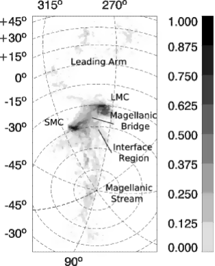
Figure 1: Contour map of the observed H I integrated relative column density in the Magellanic System. Data by Brüns et al. (Bruens05 (2005)) is projected on the plane of sky. Galactic coordinates are used.

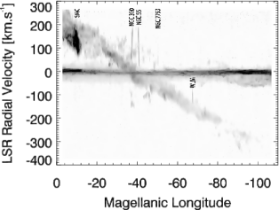
Figure 2: LSR radial velocity of the Magellanic Stream as a function of Magellanic Longitude (see Wannier & Wrixon WannierMS (1972)). The observational data by Brüns et al. (Bruens05 (2005)) is plotted. Strong H I emission observed for $\mathrm{\upsilon_{LSR}\approx 0\,km\,s^{-1}}$ comes from the MW. The map also shows the emission from the SMC, the galaxies NGC 300, NGC 55, and NGC 7793 from the Sculptor Group, and the Local Group galaxy WLM.

information about the Clouds and the connected extended structures. It indicates that the observed features consist of the matter torn off the Magellanic Clouds and spread out due to the interaction between the LMC, SMC, and MW.

2.2 Modeling of the Magellanic System

Toomre & Toomre (Toomre72 (1972)) have shown the applicability of restricted N–body models on interacting galaxies. In restricted N–body simulations, gravitating particles are replaced by test–particles moving in a time–dependent potential that is a superposition of analytic potentials of the individual galaxies. Such an approach maps the gravitational potential with high spatial resolution for low CPU costs due to the linear CPU scaling with the number of particles. However, the self–gravity of the stellar systems is not considered directly. That is, the orbital decay of the Magellanic Clouds due to dynamical friction cannot be treated self–consistently in restricted N–body simulations, but has to be considered by (semi–)analytical approximative formulas.

The first papers on the physical features of the interacting system of the LMC, the SMC and the Galaxy used 3 D restricted N–body simulations to investigate the tidal origin of the extended Magellanic structures. Lin & Lynden–Bell (Lin77 (1977)) pointed out the problem of the large parameter space of the LMC–SMC–MW interaction. To reduce the parameter space, they neglected both the SMC influence on the System and dynamical friction within the MW halo, and showed that such configuration allows for the existence of a LMC trailing tidal stream. The interaction between the Clouds was analyzed by Fujimoto & Sofue (Sofue76 (1976)), who assume the LMC and SMC to form a gravitationally bound pair for several Gyr, moving in a flattened MW halo. They identified some LMC and SMC orbital paths leading to the creation of a tidal tail. Following studies by Murai & Fujimoto (Murai80 (1980), Murai84 (1984)), Lin & Lynden–Bell (Lin82 (1982)), Gardiner et al. (Gardiner94 (1994)), and Lin et al. (Lin95 (1995)) extended and developed test–particle models of the LMC–SMC–MW interaction. The Magellanic Stream was reproduced as a remnant of the LMC–SMC encounter that was mostly placed at the time of $\mathrm{-2\,Gyr}$. The matter torn off was spread along the paths of the Clouds. The simulations also indicate that the major fraction of the Magellanic Stream gas stems from the SMC. The observed radial velocity profile of the Stream was modeled remarkably well. However, the smooth H I column density distribution did not agree with observations indicating apparently clumpy Magellanic Stream structure. Test–particle models place matter at the Leading Arm area naturally (see the study on the origin of tidal tails and arms by Toomre & Toomre (Toomre72 (1972))), but correspondence with observational data cannot be considered sufficient. Gardiner & Noguchi (Gardiner96 (1996)) devised a scheme of the Magellanic System interaction implementing the full N–body approach. The SMC was modeled by a self–gravitating sphere moving in the LMC and MW analytic potentials. It was shown that the evolution of the Magellanic Stream and the Leading Arm is dominated by tides, which supports the applicability of test–particle codes for the modeling of extended Magellanic structures. Recently, the study by Connors et al. (Connors05 (2005)) investigated the evolution of the Magellanic Stream as a process of tidal stripping of gas from the SMC. Their high–resolution N–body model of the Magellanic System based on ideas of Gardiner & Noguchi (Gardiner96 (1996)) is compared to the data from the HIPASS survey. Involving pure gravitational interaction allowed for remarkably good reproduction of the Magellanic Stream LSR radial velocity profile. They were able to improve previous models of the Leading Arm. Similarly to the previous tidal scenarios, difficulties remain concerning overestimations of the H I column density toward the far tip of the Magellanic Stream. Connors et al. (Connors05 (2005)) approximate both the LMC and the MW by rigid potentials and also do not study the influence of the non–spherical halo of the MW.

Meurer et al. (Meurer85 (1985)) involved continuous ram pressure stripping into their simulation of the Magellanic System. This approach was followed later by Sofue (Sofue94 (1994)), who neglected the presence of the SMC, however. The Magellanic Stream was formed of the gas stripped from outer regions of the Clouds due to collisions with the MW extended ionized disk. Heller & Rohlfs (Heller94 (1994)) argue for a LMC–SMC collision 500 Myr ago that established the MB. Later, gas distributed to the inter–cloud region was stripped off by ram pressure as the Clouds moved through a hot MW halo. Generally, continuous ram pressure stripping models succeeded in reproducing the decrease of the Magellanic Stream H I column density towards the far tip of the Stream. However, they are unable to explain the evidence of gaseous clumps in the Magellanic Stream. Gas stripping from the Clouds caused by isolated collisions in the MW halo was studied by Mathewson et al. (Mathewson84 (1984)). The resulting gaseous trailing tail consisted of fragments, but such a method did not allow for reproduction of the column density decrease along the Magellanic Stream. Recently, Bekki & Chiba (Bekki05 (2005)) applied a complex gas–dynamical model including star–formation to investigate the dynamical and chemical evolution of the LMC. They include self–gravity and gas dynamics by means of sticky particles, but they are also not complete: they assume a live LMC system, but the SMC and MW were treated by static spherical potentials. Thus, dynamical friction of the LMC in the MW halo is only considered by an analytical formula and a possible flattening of the MW halo is not involved. Their model cannot investigate the possible SMC origin of the Magellanic Stream either. Mastropietro et al. (Mastropietro05 (2005)) introduced their model of the Magellanic System including hydrodynamics (SPH) and a full N–body description of gravity. They studied the interaction between the LMC and the MW. Similarly to Lin & Lynden–Bell (Lin77 (1977)) and Sofue (Sofue94 (1994)), the presence of the SMC was not taken into account. It was shown that the Stream, which sufficiently reproduces the observed H I column density distribution, might have been created without an LMC–SMC interaction. However, the history of the Leading Arm was not investigated.

In general, hydrodynamical models allow for better reproduction of the Magellanic Stream H I column density profile than tidal schemes. However, they constantly fail to reproduce the Magellanic Stream radial velocity measurements and especially the high–negative velocity tip of the Magellanic Stream. Both families of models suffer from serious difficulties when modeling the Leading Arm.

To model the evolution of the Magellanic System, the initial conditions and all parameters of their interaction have to be determined. Such a parameter space becomes quite extended. In the Magellanic System we have to deal with the orbital parameters and the orientation of the two Clouds, their internal properties (like the extension of the disk), and the properties of the MW potential. In total we have about 20 parameters (the exact number depends on the adopted sophistication of the model). Previous studies of the Magellanic Clouds, however, argued for very similar evolutionary scenarios of the system (e.g., Lin & Lynden–Bell Lin82 (1982), Gardiner et al. Gardiner94 (1994), Bekki & Chiba Bekki05 (2005)). These calculations are based on additional assumptions concerning the orbits, or the internal structure and orientation of the Clouds, the potential of the MW (mass distribution and shape), the treatment of dynamical friction in the Galactic halo, or the treatment of self–gravity and gas dynamics in the Magellanic Stream. Some of them can be motivated by additional constraints. For example, Lin & Lynden-Bell (Lin82 (1982)) and Irwin et al. (Irwin90 (1990)) argue that the Clouds should have been gravitationally bound over the last several Gyr. However, in general, the uniqueness of the adopted models is unclear, because a systematic analysis of the entire parameter space is still missing.

We explore the LMC–SMC–MW interaction parameter space that is compatible with the observations of the Magellanic System available to date. Regarding the dimension and size of the parameter space, a large number of the numerical model runs have to be performed to test possible parameter combinations, no matter what kind of search technique is selected. In such a case, despite their physical reliability, full N–body models are of little use, due to their computational costs.

3 Method

To cope with the extended parameter space, neither a complete catalog of models nor a large number of computationally expensive self–consistent simulations can be performed, both due to numerical costs. However, a new numerical approach based on evolutionary optimization methods combined with fast (approximative) N–body integrators turned out to be a promising tool for such a task. In case of encounters between two galaxies, Wahde (Wahde98 (1998)) and Theis (Theis99 (1999)) showed that a combination of a genetic algorithm with restricted N–body simulations is able to reproduce the parameters of the interaction.

Here we apply the GA search strategy with a restricted N–body code for the Magellanic System. In the following sections we describe first our N–body calculations and then we briefly explain the applied genetic algorithm.

3.1 N–body simulations

Our simulations were performed by test–particle codes similar to the ones already applied to the Magellanic System by Murai & Fujimoto (Murai80 (1980)) and Gardiner et al. (Gardiner94 (1994)). But as an extension of these previous papers we allow for a flattened MW halo potential and a more exact formula for dynamical friction taking anisotropic velocity distributions into account.

For the galactic potentials we used the following descriptions: both LMC and SMC are represented by Plummer spheres. The potential of the DM halo of the MW is modeled by a flattened axisymmetric logarithmic potential (Binney & Tremaine Binney87 (1987))

$$\Phi_{\mathrm{L}}=\frac{1}{2}{\upsilon_{0}}^{2}\ln\left({R_{\mathrm{c}}}^{2}+R^{2}+\frac{z^{2}}{q^{2}}\right).$$ (1)

In agreement with Helmi (Helmi04 (2004)) we set $R_{\mathrm{c}}=12\,\mathrm{kpc}$ and $\upsilon_{0}=\sqrt{2}\cdot 131.5\,\mathrm{km\,s^{-1}}$, and $q$ describes the flattening of the MW halo potential. The corresponding flattening $q_{\rho}$ of the density distribution associated with the halo potential follows

$${q_{\rho}}^{2}=\frac{1+4q^{2}}{2+3/q^{2}}\ \ \ (R\ll R_{\mathrm{c}}),$$ (2)

$${q_{\rho}}^{2}={q}^{2}\left(2-\frac{1}{{q}^{2}}\right)\ \ \ (R\gg R_{\mathrm{c}}).$$ (3)

The choice for the logarithmic potential was motivated by several reasons. First, it allows for the investigation of flattened configurations of the Galactic halo at low computational costs. Also the relatively small number of input parameters of Eq. 1 is an advantage concerning the performance and speed of the numerical model. Finally, the logarithmic potential was employed in the recent study by Helmi (Helmi04 (2004)) that used the similar method of dwarf galaxy streams to investigate the MW DM halo, and so the application of the same formula allows for comparison of our results.

Dynamical friction causes the orbital decay of the Magellanic Clouds. We adopted the analytic dynamical friction formula by Binney (Binney77 (1977)). In contrast to the commonly used expression by Chandrasekhar (Chandra43 (1943)), it allows for an anisotropic velocity distribution. By comparison with N–body simulations of sinking satellites, Peñarrubia et al. (Pena04 (2004)) showed that Binney’s solution is a significant improvement over the standard approach with Chandrasekhar’s formula.

Finally, we get the following equations of motion of the Clouds:

$$\frac{\mathrm{d}\@vec{\upsilon}_{\mathrm{LMC}}}{\mathrm{d}t}=-(\nabla\Phi_{\mathrm{L}}+\nabla\Phi_{\mathrm{SMC}})+\frac{\@vec{F}_{\mathrm{DF}}}{m_{\mathrm{LMC}}},$$ (4)

$$\frac{\mathrm{d}\@vec{\upsilon}_{\mathrm{SMC}}}{\mathrm{d}t}=-(\nabla\Phi_{\mathrm{L}}+\nabla\Phi_{\mathrm{LMC}})+\frac{\@vec{F}_{\mathrm{DF}}}{m_{\mathrm{SMC}}},$$ (5)

where $\Phi_{\mathrm{LMC}}$, $\Phi_{\mathrm{SMC}}$ are the LMC, SMC Plummer potentials, and $\@vec{F}_{\mathrm{DF}}$ is the dynamical friction force exerted on the Clouds as they move in the MW DM halo.

Our simulations were performed with the total number of 10 000 test–particles equally distributed to both Clouds. We start the simulation with test–particles in a disk–like configuration with an exponential particle density profile, and compute the evolution of the test–particle distribution up to the present time. Initial conditions for the starting point of the evolution of the System at the time –4 Gyr were obtained by the standard backward integration of equations of motion (see, e.g., Murai &  Fujimoto Murai80 (1980), Gardiner et al. Gardiner94 (1994)). Basically, the choice for the starting epoch of this study originates in the fact that the MW, LMC, and SMC form an isolated system in our model. Such an assumption was very common in previous papers on the Magellanic System (e.g., Murai & Fujimoto Murai80 (1980), Gardiner et al. Gardiner94 (1994), Gardiner & Noguchi Gardiner96 (1996)) and was motivated by insufficient kinematic information about the Local Group, that did not allow for the estimation of the influence of its members other than MW on the evolution of the Magellanic System. Our detailed analysis of the orbits of LMC and SMC showed that the galactocentric distance of either of the Clouds did not exceed 300 kpc within the last 4 Gyr. Investigation of the kinematic history of the Local Group by Byrd et al. (Byrd94 (1994)) indicates that the restriction of the maximal galactocentric radius of the Magellanic System to $R_{\mathrm{max}}\approx 300$ kpc when $T>-4$ Gyr lets us consider the orbital motion of the Clouds to be gravitationally dominated by the MW.

3.2 Genetic algorithm search

Genetic algorithms can be used to solve optimization problems like a search in an extended parameter space. The basic concept of GA optimization is to interpret the natural evolution of a population of individuals as an optimization process, i.e., an increasing adaptation of a population to given conditions. In our case the conditions are to match numerical models to the observations. Each single point in parameter space uniquely defines one interaction scenario that can be compared with the observations (after the N–body simulation is performed). The quality of each point in parameter space (or the corresponding N–body model) can be characterized by the value of a fitness function ($FF$), which is constructed to become larger, the better the model matches the observations. A population consists of a set of points in parameter space (individuals). Each single parameter of an individual corresponds to a gene. A genetic algorithm recombines the genes of the individuals in different reproduction steps: First two individuals (parents) are selected with a probability growing with their fitness. Then the genes of the parents are recombined by application of reproduction operators mimicking cross–over and mutation. Often the reproduction is done for all members of a population. Then the newly created population corresponds to a next generation. The reproduction steps are then repeated until a given number

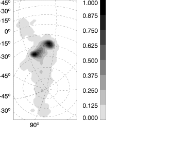
Figure 3: Contour map of the observed H I integrated column density. The original data cube by Brüns et al. (Bruens05 (2005)) is modified by frequency filtering (see Appendix B) and integrated over all radial velocity channels. The contour map is projected on the plane of sky. Galactic coordinates are used.

of generations is calculated or a sufficient convergence is reached. More details about genetic algorithms can be found in Holland (Holland75 (1975)) or Goldberg (Goldberg89 (1989)). An application to interacting galaxies is described in Wahde  (Wahde98 (1998)), Theis (Theis99 (1999)), or Theis & Kohle (Theis01 (2001)).

Obviously, the evolutionary search for the optimal solution can be treated as a process of maximizing the fitness of individuals. The GA looks for maxima of the function assigning individuals their fitness values. It should be noted that the problem we want to solve only enters via the $FF$. Therefore, the choice of the $FF$ is essential for the performance and the answer given by a GA.

For our calculations we used a $FF$ consisting of three different parts corresponding to three different comparisons. These three $FF$s measure the quality of the numerical models for different aspects of the given H I data cube. The original 3D H I data cube together with its version modified for the purpose of an efficient GA search are visualized in Fig. 20. Two of the comparisons deal with the whole data cube: $FF_{2}$ denotes the rough occupation of cells in the data cube and is a measure for the agreement of the structural shape in the data cube. $FF_{3}$ compares the individual intensities in each cell of the data cube. The $FF_{3}$ definition basically follows the $FF$ introduced in Theis (Theis99 (1999)) or Theis & Kohle (Theis01 (2001)), who found it to be an efficient GA driver for the galactic interaction problems they studied. However, if the fraction of the total volume of the system’s data cube that is occupied by the structures of special interest is small ($\mathrm{<10\%}$ in the case of the Magellanic Stream and the Leading Arm), implementation of a structural search in the data ($FF_{2}$) preceding the fine comparison between modeled and observed data significantly improves the performance of the GA. Finally, $FF_{1}$ is introduced to take into account the velocity profile, i.e., the important constraint of the minimum velocity in the stream. All these three quality measures are combined to yield the final fitness of a model. Details can be found in Appendix B.

3.3 The GA parameter space

In this paragraph we introduce the parameters of the Magellanic System interaction that were subject to our GA search. The parameters involve the initial conditions of the LMC and SMC motion, their total masses, parameters of mass distribution, particle disc radii, and orientation angles, and also the MW dark matter halo potential flattening parameter. Table 1 summarizes the parameters of the interaction and introduces their current values. Models are described in a right–handed Cartesian coordinate

Table 1: Parameters of the MW–LMC–SMC interaction.

Param.	Value
$\mathrm{\@vec{r}_{LMC}[kpc]}$	$\left(\begin{array}[]{r}\langle-1.5,-0.5\rangle\\ \langle-41.0,-40.0\rangle\\ \langle-27.1,-26.1\rangle\end{array}\right)$	Current galactocentric
		position vectors
$\mathrm{\@vec{r}_{SMC}[kpc]}$	$\left(\begin{array}[]{r}\langle 13.1,14.1\rangle\\ \langle-34.8,-33.8\rangle\\ \langle-40.3,-39.3\rangle\end{array}\right)$
$\mathrm{\@vec{\upsilon}_{LMC}[km\,s^{-1}]}$	$\left(\begin{array}[]{r}\langle-3,85\rangle\\ \langle-231,-169\rangle\\ \langle 132,206\rangle\end{array}\right)$	Current velocity
		vectors
$\mathrm{\@vec{\upsilon}_{SMC}[km\,s^{-1}]}$	$\left(\begin{array}[]{r}\langle-112,232\rangle\\ \langle-346,-2\rangle\\ \langle 45,301\rangle\end{array}\right)$
$m_{\mathrm{LMC}}\mathrm{[10^{9}M_{\odot}]}$	$\langle 15.0,25.0\rangle$	Masses
$m_{\mathrm{SMC}}\mathrm{[10^{9}M_{\odot}]}$	$\langle 1.5,2.5\rangle$
$\epsilon_{\mathrm{LMC}}\mathrm{[kpc]}$	$\langle 2.5,3.5\rangle$	Plummer sphere
$\epsilon_{\mathrm{SMC}}\mathrm{[kpc]}$	$\langle 1.5,2.5\rangle$	scale radii
$r^{\mathrm{disk}}_{\mathrm{LMC}}\mathrm{[kpc]}$	$\langle 9.0,11.0\rangle$	Particle disk radii
$r^{\mathrm{disk}}_{\mathrm{SMC}}\mathrm{[kpc]}$	$\langle 5.0,7.0\rangle$
$\Theta^{\mathrm{disk}}_{\mathrm{LMC}}$	$\langle 87^{\circ},107^{\circ}\rangle$	Disk orientation angles
$\Phi^{\mathrm{disk}}_{\mathrm{LMC}}$	$\langle 261^{\circ},281^{\circ}\rangle$
$\Theta^{\mathrm{disk}}_{\mathrm{SMC}}$	$\langle 35^{\circ},55^{\circ}\rangle$
$\Phi^{\mathrm{disk}}_{\mathrm{SMC}}$	$\langle 220^{\circ},240^{\circ}\rangle$
$q$	$\langle 0.74,1.20\rangle$	MW DM halo
		potential flattening

system with the origin in the Galactic center. This system is considered to be an inertial frame because we assume that $m_{\mathrm{MW}}\gg m_{\mathrm{LMC}},m_{\mathrm{SMC}}$, where $m_{\mathrm{MW}}$ is the mass of MW, and $m_{\mathrm{LMC}}$ and $m_{\mathrm{SMC}}$ are the masses of LMC and SMC, respectively. Therefore, the center of mass of the system may be placed at the Galactic center. We assume the present position vector of the Sun $\mathrm{\@vec{R_{\odot}}=(-8.5,0.0,0.0)\,kpc}$. In the following paragraphs we will discuss the parameters of the LMC–SMC–MW interaction and the determination of their ranges.

The nature and distribution of dark matter in the Galaxy has been subject to intense research and a large number of models have been proposed. We probe the DM matter distribution by investigating the redistribution of matter in the Magellanic System due to the MW–LMC–SMC interaction, paying special attention to the features of the Magellanic Stream. That is similar to the method applied by Helmi (Helmi04 (2004)), who studied kinematic properties of the Sagittarius stream. To enable comparison with the results by Helmi (Helmi04 (2004)), we also adopted the axially symmetric logarithmic halo model of MW (Eq. 1) and the same values of the halo structural parameters $R_{\mathrm{c}}$, and $\upsilon_{0}$ with a similar range of studied values of the flattening $q$ (see Table 1). We extended the range of $q$ values tested by Helmi (Helmi04 (2004)) to the lower limit of $q=0.74$, which is the minimal value acceptable for the model of a logarithmic halo (for a detailed explanation see Binney & Tremaine (Binney87 (1987))). For every value of $q$, a time–consuming calculation of parameters of dynamical friction is required (see Appendix A). To reduce the computational difficulties, the flattening $q$ was treated as a discrete value with a step of $\Delta q=0.02$, and the parameters of dynamical friction were tabulated. The upper limit of $q=1.20$ was selected to enable testing of prolate halo configurations. Extension of the halo flattening range to higher values was not considered due to the computational performance limits of our numerical code.

The estimated ranges of the values of the remaining parameters are based on our observational knowledge in the Magellanic System. Galactocentric position vectors $\@vec{r}_{\mathrm{LMC}}$ and $\@vec{r}_{\mathrm{SMC}}$ agree with the LMC and SMC distance moduli measurements given by Van den Bergh (Vandenbergh00 (2000)), who derived the mean values of distance moduli $\overline{(m-M)}_{0}=18.50\pm 0.05$ for LMC and $\overline{(m-M)}_{0}=18.85\pm 0.1$ for SMC, corresponding to the heliocentric distances of $\mathrm{(50.1\pm 1.2)\,kpc}$ and $\mathrm{(58.9\pm 2.6)\,kpc}$, respectively. Only 2 of the 6 components of the LMC and SMC position vectors enter the GA search as free parameters because the rest of them are determined by the projected position of the Clouds on the plane of sky, that is $l_{LMC}=280^{\circ}\,27^{\prime}$, $b_{\mathrm{LMC}}=-32^{\circ}\,53^{\prime}$ and $l_{\mathrm{SMC}}=302^{\circ}\,47^{\prime}$, $b_{\mathrm{SMC}}=-44^{\circ}\,18^{\prime}$.

Previous studies by Murai & Fujimoto (Murai80 (1980)) and Gardiner et al. (Gardiner94 (1994)) found that the correct choice of the spatial velocities is crucial for reproducing the observed H I structures. Kroupa & Bastian (Kroupa97 (1997)) derived proper motions of LMC and SMC stars from an analysis of HIPPARCOS such that $\mathrm{\@vec{\upsilon}_{LMC}=(+41\pm 44,-200\pm 31,+169\pm 37)\,km\,s^{-1}}$ and $\mathrm{\@vec{\upsilon}_{SMC}=(+60\pm 172,-174\pm 172,+173\pm 128)\,km\,s^{-1}}$. The large uncertainties in actual values of the LMC and SMC velocity vectors originate in the fact that the measured transverse velocities suffer from large rms errors, which is connected to the large distance of LMC and SMC in combination with the limited precision of proper motions in the HIPPARCOS catalog. To derive the actual initial conditions at the starting time of the simulation from the current positions and velocities of the Clouds, we employed the backward integration of equations of motion.

Current total masses $m_{\mathrm{LMC}}$ and $m_{\mathrm{SMC}}$ follow estimates by Van den Bergh (Vandenbergh00 (2000)). In general, masses of the Clouds are functions of time and evolve due to the LMC–SMC exchange of matter, and as a consequence of the interaction between the Clouds and MW. Our test–particle model does not allow for a reasonable treatment of a time–dependent mass–loss. Therefore, masses of the Clouds are considered constant in time, and their initial values at the starting epoch of our simulations are approximated by the current LMC and SMC masses. Regarding the large range of the LMC and SMC mass estimates available (for details see Van den Bergh (Vandenbergh00 (2000))), $m_{\mathrm{LMC}}$ and $m_{\mathrm{SMC}}$ are also treated as free input parameters of our model that become subjects to the GA optimization. Their ranges that we investigated can be found in Table 1.

Scale radii of the LMC and SMC Plummer potentials $\epsilon_{\mathrm{LMC}}$ and $\epsilon_{\mathrm{SMC}}$ are input parameters of the model describing the radial mass distribution in the Clouds. The study by Gardiner et al. (Gardiner94 (1994)) used the values $\epsilon_{\mathrm{LMC}}=3$ kpc and $\epsilon_{\mathrm{SMC}}=2$ kpc. To investigate the influence of this parameter on the evolution of the Magellanic System, the Plummer radii were involved in the GA search and their values were varied within the ranges of the width of 1 kpc, including the estimates by Gardiner et al. (Gardiner94 (1994)) (see Table 1).

Gardiner et al. (Gardiner94 (1994)) analyzed the H I surface contour map of the Clouds to estimate the initial LMC and SMC disk radii entering their model of the Magellanic System as initial conditions. Regarding the absence of a clearly defined disk of the SMC, and possible significant mass redistribution in the Clouds during their evolution, the results require careful treatment and further verification. We varied the current estimates of disk radii $r^{\mathrm{disk}}_{\mathrm{LMC}}$ and $r^{\mathrm{disk}}_{\mathrm{SMC}}$ as free parameters within the ranges introduced in Table 1, containing the values derived by Gardiner et al. (Gardiner94 (1994)), and used them as initial values at the starting point of our calculations ($T=-4$ Gyr).

The orientation of the disks is described by two angles $\Theta$ and $\Phi$ defined by Gardiner & Noguchi (Gardiner96 (1996)). Several observational determinations of the LMC disk plane orientation were collected by Lin et al. (Lin95 (1995)). Its sense of rotation is assumed to be clockwise (Lin et al. Lin95 (1995), Kroupa & Bastian Kroupa97 (1997)). The position angle of the bar structure in the SMC was used by Gardiner & Noguchi (Gardiner96 (1996)) to investigate the current disk orientation. Their results allow for wide ranges of the LMC and SMC disk orientation angles (see Table 1) and so we investigated $\Theta$ and $\Phi$ by the GA search method, too. Similarly to Gardiner & Noguchi (Gardiner96 (1996)), we use the current LMC and SMC disk orientation angles (Table 1) to approximate their initial values at $T=-4$ Gyr.

4 Results

We try to reproduce as closely as possible the column density and velocity distribution of H I in the Magellanic Stream and in the Leading Arm. The influence of actual distances to the LMC and SMC and of their present space velocity vectors is considered together with their masses and the past sizes and space orientations of the orginal disks. Here, we give the results of the search in the parameter space with the GA using the 3–component $FF$ defined by Eq. 10. In principle, the GA is able to find the global extreme of the FF if enough time is allowed for the evolution of the explored system (see Holland Holland75 (1975)). However, it may be very time–consuming to identify the single best fit due to a slow convergence of the FF. Therefore, to keep the computational cost reasonable, the maximum number of 120 GA generations to go through was defined.

To explore the $FF$ of our system, we collected 123 GA fits of the Magellanic System resulting from repeated runs of our GA optimizer. Typically, identification of a single GA fit requires $\mathrm{\approx 10^{4}}$ runs of the numerical model. Thus, due to the application of GA we were able to search the extended parameter space of the interaction and discover the most successful models of the System over the entire parameter space by testing $\mathrm{\approx 10^{6}}$ parameter combinations. In the case of our 20–dimensional parameter space, simple exploration of every possible combination of parameters even on a sparse grid of, e.g., 10 nodes per dimension, means $\mathrm{10^{20}}$ runs of the model. Such a comparison clearly shows the necessity of using optimization techniques and demonstrates computational efficiency of GA.

Figure 4: Maximum values of fitness as a function of the MW dark matter halo flattening $q$. The plot depicts the fitness of the best GA fit of the Magellanic System that was found for each of the MW dark matter halo flattening values that entered the GA search. The function is also approximated by its least–square polynomial fit. The values of $q$ delimiting the model groups A, B, and C (see Table 2) are emphasized by dotted lines.

The fitness distribution for different values of the halo flattening parameter $q$ is shown in Fig. 4. For every value of $q$, the model of the highest fitness is selected and its fitness value is plotted. Figure 4 indicates that better agreement between the models and observational data was generally achieved for oblate halo configurations rather than for nearly spherical or prolate halos. The relative difference between the worst ($Fit_{\mathrm{MIN}}=0.450;q=1.14$) and the best ($Fit_{\mathrm{MAX}}=0.496;q=0.84$) model shown in Fig. 4 is $\Delta Fit=0.09$. It reflects the fact that each of the GA fits contains a trailing tail (Magellanic Stream) and a leading stream (Leading Arm), but that there are fine differences between the resulting distributions of matter. One may note that the GA optimizer did not discover a model of fitness over 0.5 (the maximum reachable fitness value is 1.0 – see Appendix B). It is caused either by insufficient volume of the studied parameter space of the interaction, or by simplification of physical processes in our model (see Sec. 6), or by a combination of both reasons. That establishes an interesting problem and should become a subject to future studies.

We want to discuss our results with respect to the shape of the MW halo.

Table 2: Three major groups according to the halo flattening $q$

Group	A	B	C
	$0.74\leq q\leq 0.92$	$0.94\leq q\leq 1.06$	$1.08\leq q\leq 1.20$
$N_{i}$	101	10	12

Thus, all the GA fits are divided into three groups according to the halo flattening (see Table 2) to show differences or common features of models for oblate, nearly spherical, and prolate halo configurations. The actual borders between the groups A, B, and C were selected by definition and, so that the number of models in each of the groups allows for statistical treatment of the LMC and SMC orbital features and particle redistribution that will be introduced in Sect. 4.1.

4.1 Evolution

Figure 5: Relative numbers of the Magellanic System GA models with LMC–SMC relative distance minima at a given time interval for model groups A (left), B (middle), and C. The counts were made for 8 time intervals of 500 Myr covering the entire Magellanic evolution period of 4 Gyr investigated in our study.

Figure 6: Mean values of the LMC–SMC distance minima for model groups A (left), B (middle), and C (Table 2) and for 8 time intervals of 500 Myr.

Figure 7: Relative number of the LMC and SMC test–particles strongly disturbed due to the Magellanic System interaction. Counts within 8 time intervals of 500 Myr and for model groups A (left), B (middle), and C are plotted.

Close encounters of interacting galaxies often lead to substantial disruption of their particle disks, forming subsequently tidal arms and tails (Toomre & Toomre Toomre72 (1972)). Regarding that, the time dependence of the relative distance of the interacting pair is an interesting source of information about the system.

First of all, we examine the time distribution of the minima of the LMC–SMC relative distance. For each of the model groups mentioned in Table 2, we calculate the relative number of GA solutions having a minimum of the LMC–SMC relative distance within a given interval of 500 Myr. Figure 5 shows such a distribution of fits for the total time interval of our simulations, which is 4.0 Gyr. The local maxima of the time distribution of the LMC–SMC distance minima are within the intervals $\mathrm{\langle-3.0,-2.0\rangle\,Gyr}$ and $\mathrm{\langle-0.5,0.0\rangle\,Gyr}$. For prolate halos ($q\geq 1.08$) there is no LMC–SMC distance minimum between -2.0 Gyr and -0.5 Gyr.

Subsequently, the mean values of the LMC–SMC distance minima are calculated for each of the time intervals defined above. Comparison of the results for oblate, nearly spherical, and prolate DM halo configuration is available in Fig. 6. It was found that close ($\Delta r\approx 10$ kpc) LMC–SMC encounters do not occur in models with either oblate or prolate halos. If the MW DM halo shape is nearly spherical, disruption of the LMC and SMC initial particle distribution leading to creation of the observed H I structures typically occurred due to strong LMC–SMC interaction.

Another point of interest is the time dependence of the LMC and SMC test–particle redistribution during the evolutionary process. Figure 7 offers the relative number of test–particles strongly disturbed, i.e., particles that reached the minimal distance of twice the original radii of their circular orbits around the LMC and SMC centers, respectively, and by the LMC–SMC–MW interaction in the defined time–intervals. Comparison between the plots in Figs. 6 and 7 shows that encounters of the Clouds are followed by delayed raise of the number of particles shifted to different orbits, typically. Another such events are induced by the interaction of the Clouds and MW. Disruption of the LMC and SMC disks triggers formation of the extended structures of the Magellanic System. Particles are assigned new orbits in the superimposed gravitational potential of the LMC, SMC, and MW, and spread along the orbital paths of the Clouds. Our study shows that the formation of the Magellanic Stream and other observed H I features did not begin earlier than 2.5 Gyr ago for model groups A and B (see Fig. 7). Prolate halos (group C) allow for a mass redistribution in the system that started at $T<-3.5$ Gyr.

4.2 Representative models

Here, we describe the models of highest fitness selected from each of the groups A, B, and C. All of them are typical representatives of their model groups and we discuss

Table 3: Parameters of the best models in separate $q$ categories.

Model	A	B	C
$q$	0.84	1.02	1.16
$Fit$	0.496	0.467	0.473
$\mathrm{\@vec{r}_{LMC}[kpc]}$	$\left(\begin{array}[]{r}-1.26\\ -40.50\\ -26.87\end{array}\right)$	$\left(\begin{array}[]{r}-0.90\\ -40.31\\ -26.88\end{array}\right)$	$\left(\begin{array}[]{r}-0.63\\ -40.03\\ -26.92\end{array}\right)$
$\mathrm{\@vec{r}_{SMC}[kpc]}$	$\left(\begin{array}[]{r}13.16\\ -34.26\\ -39.77\end{array}\right)$	$\left(\begin{array}[]{r}13.32\\ -34.33\\ -40.22\end{array}\right)$	$\left(\begin{array}[]{r}13.92\\ -34.04\\ -39.86\end{array}\right)$
$\mathrm{\@vec{\upsilon}_{LMC}[km\,s^{-1}]}$	$\left(\begin{array}[]{r}44.0\\ -169.8\\ 146.7\end{array}\right)$	$\left(\begin{array}[]{r}18.5\\ -169.3\\ 171.3\end{array}\right)$	$\left(\begin{array}[]{r}5.8\\ -169.2\\ 205.8\end{array}\right)$
$\mathrm{\@vec{\upsilon}_{SMC}[km\,s^{-1}]}$	$\left(\begin{array}[]{r}-37.2\\ -60.2\\ 204.3\end{array}\right)$	$\left(\begin{array}[]{r}-10.1\\ -94.2\\ 270.0\end{array}\right)$	$\left(\begin{array}[]{r}-47.5\\ -13.2\\ 162.6\end{array}\right)$
$m_{\mathrm{LMC}}[10^{9}\mathrm{M_{\odot}}]$	24.46	19.86	19.01
$m_{\mathrm{SMC}}[10^{9}\mathrm{M_{\odot}}]$	2.06	1.82	1.83
$r^{\mathrm{disk}}_{\mathrm{LMC}}\mathrm{[kpc]}$	9.62	11.46	9.06
$r^{\mathrm{disk}}_{\mathrm{SMC}}\mathrm{[kpc]}$	6.54	6.06	7.90
$\Theta^{\mathrm{disk}}_{\mathrm{LMC}}$	$89^{\circ}$	$98^{\circ}$	$102^{\circ}$
$\Phi^{\mathrm{disk}}_{\mathrm{LMC}}$	$274^{\circ}$	$277^{\circ}$	$281^{\circ}$
$\Theta^{\mathrm{disk}}_{\mathrm{SMC}}$	$36^{\circ}$	$49^{\circ}$	$36^{\circ}$
$\Phi^{\mathrm{disk}}_{\mathrm{SMC}}$	$229^{\circ}$	$231^{\circ}$	$224^{\circ}$

their features with respect to the H I observational data. Table 3 summarizes the parameter values of the models.

4.2.1 Group A

The best model of the Magellanic System with an oblate MW halo is introduced in this section (model A). Figure 8 depicts the time variation of the LMC and SMC galactocentric distances together with the LMC–SMC separation for the last 4 Gyr. The Clouds move on very different orbits. The apogalactic distance of LMC decreases systematically during the evolutionary period, which clearly reflects the effect of dynamical friction. There is a gap between the periods of subsequent perigalactic approaches of the Clouds. While the last two perigalactica of LMC are separated by $\mathrm{\approx 2.3\,Gyr}$, it is not over $\mathrm{\approx 1.5\,Gyr}$ in the case of the SMC. Filled parts of the plot in Fig. 8 indicate that the Magellanic Clouds have reached the state of a gravitationally bound system during the last 4 Gyr. We define gravitational binding by the sum of the relative kinetic and gravitational potential energy of LMC and SMC. The Clouds are bound when the total energy is negative. Specifically, LMC and SMC have been forming a bound couple since $T=-1.06$ Gyr. Nevertheless, the total lifetime of a bound LMC–SMC pair did not exceed $\mathrm{40\,\%}$ of the entire evolutionary period we studied.

Comparison between Figs. 8 and 9 allows for conclusions about major events that initialized the redistribution of the LMC and SMC particles. The most significant change of the initial distribution of particles occurred as a result of the LMC–MW approach at $T\approx-2.4$ Gyr, and the preceding LMC–SMC encounter $T\approx-2.5$ Gyr. Later on, the particle redistribution continued due to tidal stripping by the MW.

Figure 10 shows the modeled distribution of integrated H I column density in the System. To enable comparison with the observed H I distribution, we plotted a normalized H I column density map. The technique used to convert a test–particle distribution into a smooth

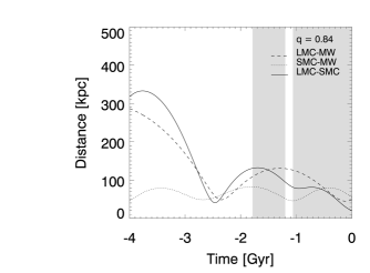
Figure 8: Orbital evolution of the Clouds for the best GA fit from the model group A. The plot corresponds to an oblate halo of flattening $q=0.84$. Time dependence of the LMC (dashed line) and SMC (dotted line) galactocentric distances, and the LMC–SMC relative distance are plotted above. Plot areas with grey filling mark the time intervals when the Clouds were gravitationally bound to each other.

map of column densities is described in Appendix B. Mass distribution of H I extends beyond the far tip of the observed Magellanic Stream (Fig. 3) in the model A. H I column density peaks can be found in Fig. 3 at the positions $l=300^{\circ}$, $b=-65^{\circ}$ and $l=45^{\circ}$, $b=-82^{\circ}$. The model A places local density maxima of H I close to those observed ones

Figure 9: Model A. Relative number of LMC/SMC test–particles strongly disturbed due to the interaction in the Magellanic System. Counts within 8 time intervals of 500 Myr are plotted.

(i.e., relative angular distance is $\approx 10^{\circ}$) to approximate positions $l=325^{\circ}$, $b=-70^{\circ}$ and $l=70^{\circ}$, $b=-70^{\circ}$, respectively. Note also the low–density distribution of matter spread along the great circle of $l=270^{\circ}$ (Fig. 10). The matter emanates from LMC near the position of the Interface Region identified by Brüns et al. Bruens05 (2005) (Fig. 1). In general, the model overestimates the amount of matter in the Magellanic Stream. The Leading Arm consists only of LMC particles in this scenario. The modeled matter distribution covers a larger area of the plane of sky than what is observed.

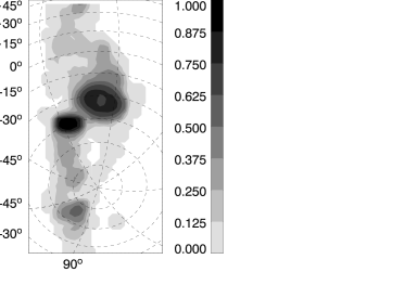
Figure 10: Model A. Contour map of the modeled H I integrated relative column density. Data is projected on the sky plane. Galactic coordinates are used.

However, this is a common problem of previous test–particle models of the Magellanic System (see, e.g., Murai & Fujimoto Murai80 (1980), Gardiner et al. Gardiner94 (1994)) and is likely caused by simplifications in the treatment of the physical processes. But also in general, successful reproduction of the Leading Arm has been a difficult task for all the models introduced so far.

The LSR radial velocity profile of the Magellanic Stream for the model A is shown in Fig. 11. The model reproduces the LSR radial velocity of the Stream matter as an almost linear function of Magellanic Longitude with the high–negative velocity tip reaching $\mathrm{-400\,km\,s^{-1}}$. Such features are in agreement with observations (see Fig. 2). In contrast to Gardiner et al. (Gardiner94 (1994)), the Magellanic Stream consists of both LMC and SMC particles. Figure 11 denotes that the

Figure 11: Model A. LSR radial velocity profile of the Magellanic Stream.

LMC and SMC Stream components cover different ranges of LSR radial velocities. The Stream component of the SMC origin does not extend to LSR radial velocities below the limit of $\mathrm{-200\,km\,s^{-1}}$. The major fraction of the LMC particles resides in the LSR radial velocity range from $\mathrm{-400\,km\,s^{-1}}$ to $\mathrm{-200\,km\,s^{-1}}$.

4.2.2 Group B

The best model of the group B (model B) corresponds to the MW DM halo flattening value $q=1.02$. The initial condition set for the model B is listed in Table 3. The galactocentric distance of the Clouds and their spatial separation as functions of time are plotted in Fig. 12. Continuous decrease of the LMC and SMC galactocentric distances due to the dynamical friction is apparent for both LMC and SMC.

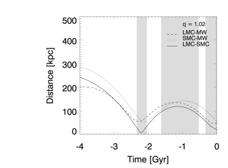
Figure 12: Orbital evolution of the Clouds for the best GA fit from the model group B. The plot corresponds to a nearly spherical halo of flattening $q=1.02$. Time dependence of the LMC (dashed line) and SMC (dotted line) galactocentric distances, and the LMC–SMC relative distance are plotted above. Grey filled areas show time intervals when the LMC and SMC formed a gravitationally bound couple.

A very close encounter of the Clouds with the relative distance $\Delta r\approx 10$ kpc occurred at $T\approx-2.2$ Gyr. At similar moments of $T\approx-2.3$ Gyr (LMC) and $T\approx-2.1$ Gyr (SMC), the Clouds also reached perigalactica of their orbits. In general, both Clouds have been moving on orbits showing similar time dependence of their galactocentric distances, as indicated by Fig. 12. Nevertheless, the position vectors of the Clouds evolved in significantly different ways. As a consequence, the spatial separation of the Clouds varied within a wide range of values from $\Delta r\approx 10$ kpc to $\Delta r\approx 250$ kpc. The Clouds have formed a gravitationally bound couple three times within the last 4 Gyr, and the total duration of such periods was 1.7 Gyr. Currently, LMC and SMC are gravitationally bound in the model B.

The LMC–SMC encounter at $T\approx-2.2$ Gyr caused a distortion of the original particle disks of the Clouds. More than $\mathrm{25\,\%}$ of the total number of the LMC and SMC particles were moved to significantly different orbits (for a definition see Sect. 4.1) within the interval of 1 Gyr after the encounter (see Fig. 13).

Figure 13: Model B. Relative number of LMC/SMC test–particles strongly disturbed due to the interaction in the Magellanic System. Counts within 8 time intervals of 500 Myr are plotted.

The following evolution of the particle distribution formed extended structures depicted in Fig. 14.

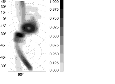
Figure 14: Model B. Contour map of the modeled H I integrated relative column density. Data is projected on the plane of sky. Galactic coordinates are used. The dominant branch of the trailing stream is along the great circle denoted by $l=135^{\circ}/315^{\circ}$.

There are two spatially separated components present in the modeled tail. The H I column density distribution map for the model B (see Fig. 14) shows a densely populated trailing stream parallel to the great circle of $l=135^{\circ}/315^{\circ}$. It consists of the SMC particles torn off from the initial disk $\mathrm{\approx 2\,Gyr}$ ago. Its far end is projected to the plane of sky close to the tip of the Magellanic Stream. However, the modeled increase of the column density of matter toward the far end of the tail is a substantial drawback of scenario B. The stream extends into the SMC leading arm located between $l=290^{\circ},b=-15^{\circ}$ and $l=290^{\circ},b=45^{\circ}$. The second component of the particle tail is of LMC origin and is spread over the position of the observed low–density gas distribution centered at $l=80^{\circ}$, $b=-50^{\circ}$ (Figs. 1 or 3).

The most significant structure at the leading side of the Magellanic System is the SMC stream introduced in the previous paragraph. Comparison between Figs. 3 and 14 indicates that neither the projected position nor the

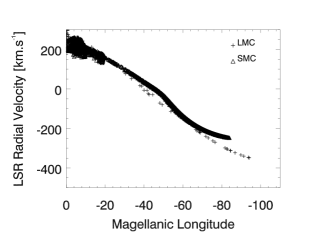
Figure 15: Model B. LSR radial velocity profile of the Magellanic Stream.

integrated H I density distribution of the stream is in agreement with the observed Leading Arm. There was also a structure emanating from the leading edge of the LMC identified at approximate position $l=270^{\circ},b=-15^{\circ}$ (see Fig. 14). Regarding the H I data by Brüns et al. (Bruens05 (2005)), such an H I distribution is not observed. The LSR radial velocity profile of the trailing tail of the model B does not extend over the limit of $\mathrm{\upsilon_{LSR}\approx-350\,km.s^{-1}}$ (Fig. 15). However, following the H I data, the far tip of the Stream should reach the LSR radial velocity $\mathrm{\upsilon_{LSR}\approx-400\,km.s^{-1}}$ at the Magellanic Longitude $\mathrm{\approx-100^{\circ}}$.

4.2.3 Group C

Our last model group C assumes the presence of prolate MW DM halos. The best GA fit of the System (model C) is introduced in Table 3 reviewing its initial condition set. Concerning orbital motion of the Clouds, there is significant difference between the LMC and SMC periods of perigalactic approaches during the last 4 Gyr.

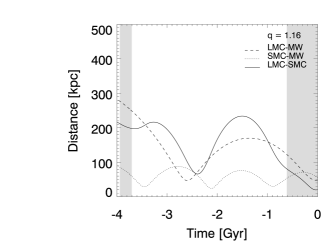
Figure 16: Orbital evolution of the Clouds for the best GA fit from the model group C. The plot corresponds to a prolate halo of flattening $q=1.16$. Time dependence of the LMC (dashed line) and SMC (dotted line) galactocentric distances, and the LMC–SMC relative distance are plotted above. Periods when the Clouds formed a gravitationally bound couple are marked by grey filling.

While the last period of the LMC exceeds 2.5 Gyr, the SMC orbital cycle is shorter than 1.5 Gyr. The relative distance of the Clouds remains over 70 kpc for $T<-0.4$ Gyr. They became a gravitationally bound couple 0.6 Gyr ago and this binding has not been disrupted (Fig. 16).

Figure 17: Model C. Relative number of LMC/SMC test–particles strongly disturbed due to the interaction in the Magellanic System. Counts within 8 time intervals of 500 Myr are plotted.

Changes to the original LMC and SMC particle disks occurred especially due to the LMC–MW and SMC–MW encounters at $T<-2.0$ Gyr. Comparison between Figs. 16 and 17 demonstrates the significance of different encounter events for particle redistribution. Note that the rise of the number of disturbed particles is delayed with respect to the corresponding disturbing event. Subsequently, the evolution of particle structures continued under the influence of tidal stripping by the gravitational field of MW. The current distribution of matter in the model C is plotted in the form of a 2–D map in Fig. 18.

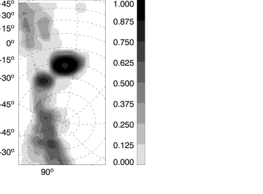
Figure 18: Model C. Contour map of the modeled H I integrated relative column density. Data is projected on the sky plane. Galactic coordinates are used.

The projection of the modeled trailing stream indicates that it occupies larger area of the data cube than the observed Magellanic Stream (compare Figs. 3 and 18). According to Fig. 3 the Magellanic Stream shows H I density peaks at $l=300^{\circ}$, $b=-65^{\circ}$ and $l=45^{\circ}$, $b=-82^{\circ}$. Our model C expects two local maxima of H I integrated column density in the tail. Their positions are shifted by $\mathrm{\approx 20^{\circ}}$ relatively to the peaks in Fig. 3. Additional comparison between the model and observations reveals that the model C overestimates the integrated column densities of H I in the Magellanic Stream. The matter located at the leading side of the Magellanic System is of SMC origin only. Similarly to the case of the trailing tail, the modeled amount of matter exceeds observational estimates for the Leading Arm.

Figure 19 offers the LSR radial velocity profile of the Magellanic Stream in our model C. The measured minimum of the LSR radial

Figure 19: Model C. LSR radial velocity profile of the Magellanic Stream.

velocity is $\mathrm{\approx-400\,km\,s^{-1}}$. The high negative LSR radial velocity at the far tip of the modeled Magellanic Stream does not exceed $\mathrm{\approx-300\,km\,s^{-1}}$, however. The observed H I emission intensity decreases towards the high negative velocity tip, which was not well reproduced by the model C.

5 Summary of the GA models

5.1 Orbits of the Magellanic Clouds

Exploration of the orbital motion of the Clouds shows the similarity of the GA fits for oblate and prolate halos (models A and C). No close ($r<10$ kpc) LMC–SMC encounters occurred for either of the models A and C. It is also notable that in the models with aspherical halos, the SMC period of perigalactic approaches is significantly shorter than the period of the LMC and that the SMC remains closer than 100 kpc to the MW center during the last 4 Gyr. When the MW DM flattening $q\approx 1.0$, the LMC and SMC orbital cycle lengths were comparable for the model B. Independently of the MW halo shape, the LMC and SMC are currently forming a gravitationally bound couple in our models. However, the Clouds cannot be considered bound to each other during the entire period of the last 4 Gyr. This is in contrast with Murai & Fujimoto (Murai80 (1980)), Gardiner et al. (Gardiner94 (1994)), or Gardiner & Noguchi (Gardiner96 (1996)), who argue that the LMC and SMC moving in the spherical halo have formed a gravitationally bound pair for at least several Gyr to allow for sufficient matter redistribution. We show that the structural resolution adopted by the above–cited studies to make a comparison between models and observations does not allow for such constraints of the orbital history of the Clouds. The GA search employed a 3–level detailed evaluation of the modeled H I distribution with respect to high–resolution observational data (Brüns et al. Bruens05 (2005)), which introduced significant improvement of previous approaches to compare observations and models. Nevertheless, there is still no clear indication that continuous gravitational binding of the Clouds covering the entire evolutionary period is necessary for successful reproduction of the observed data.

5.2 Origin of the matter in the Stream

In our best model both SMC and LMC particles were present in the trailing stream. This is a common feature of the scenarios that were investigated. In general, the fraction of H I gas originating at the SMC exceeds the fraction of LMC matter in the Stream.

Following the models A and B, the formation of the Magellanic Stream did not start earlier than 2.5 Gyr ago. In the case of the models C, the age of the Stream is $\mathrm{\approx 3.5\,Gyr}$. The estimates by the models A and B are close to the epoch when a massive star formation burst in LMC began (Van den Bergh Vandenbergh00 (2000)). It is also true for the model C. However, the disturbing event that triggered the formation of the Magellanic Stream in the model C occurred at a time that does not substantially differ from the epoch $T=-4$ Gyr when our simulation started. In such a case we have to assume that the tidal interaction responsible for the creation of the Stream was very likely invalidating the natural condition of sufficient isolation of the Clouds at the starting point of the simulation. Such a condition is necessary to set up the initial particle disks around LMC and SMC when the particles reside on circular orbits. Thus, the statements on the actual age of the Stream in the model C should be made with care. Regardless, the large uncertainty of the estimated beginning of the LMC star burst (see Van den Bergh Vandenbergh00 (2000)) requires that consideration is given to the possibility that for case A, B, or C the starting epochs of the Stream creation and of the start formation burst in the LMC may overlap.

The previous paragraph indicates that it is very likely that matter forming the Stream comes from the Magellanic Clouds containing stars, and we necessarily face the observational fact that there is no stellar content in the Magellanic Stream. The models for aspherical halos indicate that the matter coming to the Magellanic Stream from the LMC originates in the outer regions of its initial particle disk, while no matter was torn off from the inner disk of radius $\mathrm{r_{disk}\approx 5\,kpc}$ that was the dominant region of star formation in the LMC. It is due to the absence of close encounters in the Magellanic System.

In contrast to the models A and C, a dramatic encounter event between the Clouds occurred in model B at $\mathrm{\approx-2.2\,Gyr}$, when the internal structure of both disks was altered and the matter from central areas of the LMC disk was also transported to the Magellanic Stream. In such a case we expect a certain fraction of the matter of the Magellanic Stream to be in the form of stars, which is, however, not supported by observations.

5.3 Structure of the Stream

Mathewson et al. (Mathewson77 (1977)) observationally mapped the Magellanic Stream and discovered its clumpy structure consisting of six major H I clouds named MS I–VI. Recently, a more sensitive high–resolution H I survey of the Magellanic System by Brüns et al. (Bruens05 (2005)) showed that the above mentioned fragments of the Stream have to be considered density peaks of an otherwise smooth distribution of neutral hydrogen with a column density decreasing towards the high–negative radial velocity tip of the Magellanic Stream. Our models corresponding to aspherical MW halos (A, C) placed local density maxima of H I close to the South Galactic pole. That result is supported by observations by Brüns et al. (Bruens05 (2005)). In this respect, model B did not succeed, and its projected distribution of H I in a trailing tail cannot be considered a satisfactory fit of the Magellanic Stream.

Our models overestimate the integrated relative column densities of H I in the part of the Magellanic Stream located between the South Galactic pole and the far tip of the Stream. There is also no indication of the H I density decrease as we follow the Stream further from the Magellanic Clouds. In general, all of the models A, B, and C predict the trailing tail to be of higher H I column densities and extended well beyond the far tip of the Magellanic Stream. Such behavior is a common feature of pure tidal evolutionary models of the Magellanic System and it is a known drawback of omitting dissipative properties of the gaseous medium.

Regarding the LSR radial velocity measurements along the Magellanic Stream by Brüns et al. (Bruens05 (2005)), our models were able to reproduce some of their results. The far tip of the Magellanic Stream in model A reaches the extreme negative LSR radial velocity of $\mathrm{-400\,km\,s^{-1}}$ known from H I observations. However, the highest negative LSR radial velocity does not drop below $\mathrm{-350\,km\,s^{-1}}$ for either prolate or nearly spherical halo configurations. Our previous discussion of various models of the Magellanic System denoted that the successful reproduction of the high–negative LSR radial velocity at the far tip of the Magellanic Stream is one of the most challenging problems for such studies. Regarding our results, the importance of the correct LSR radial velocity profile along the Magellanic Stream was emphasized again. The absence of H I between LSR radial velocities of $\mathrm{\approx-350\,km\,s^{-1}}$ and $\mathrm{\approx-400\,km\,s^{-1}}$ turned out to be the crucial factor decreasing the resulting fitness of examined evolutionary scenarios. Based on the study of debris of the Sagittarius dwarf galaxy, Law et al. (Law05 (2005)) conclude that the velocity gradient along the trailing stream provides a sensitive evidence for the mass of the MW within 50 kpc and for the oblate shape of the galactic halo. However, the leading debris provide a contradictory evidence in favor of its prolate shape.

5.4 Leading Arm

Reproduction of the Leading Arm remains a difficult task for all the models of the Magellanic System that have been employed so far. Tidal models naturally place matter to the leading side of the System, towards the Galactic equator, as a result of the tidal stripping also forming the trailing tail. However, neither the projected shape of the modeled leading structures nor the H I density distribution in the regions having an observational counterpart can be considered sufficient (see, e.g., Gardiner et al. Gardiner94 (1994)).

In every case A, B, and C, we were able to transport matter to the area of the Leading Arm. Nevertheless, the projected coverage of that region was more extended than what is observed. All the models contain a significant content of matter spread from the leading edge of LMC across the Galactic equator, which has not been confirmed observationally. The model C reproduced the Leading Arm best. But the column density values of H I in C are overestimated and we also could not avoid an additional low–density envelope surrounding the structure (Fig. 18).

6 Uncertainties in our modeling

6.1 Missing physics

To optimize performance of the GA, a computationally fast model of the Magellanic System is required. Therefore, complex N–body schemes involving self–consistent descriptions of gravity and hydrodynamics (see Bekki & Chiba Bekki05 (2005), Mastropietro et al. Mastropietro05 (2005)) are discriminated. On the other hand, a correct description of physical processes dominating the evolution of the System remains a crucial constraint on the model.

In Sect. 2.2 we discussed the applicability of restricted N–body schemes on problems of galactic encounters and showed that they allow for modeling of extended streams and tails. Thus, we devised a restricted N–body code based on the numerical models by Murai & Fujimoto (Murai80 (1980)) and Gardiner et al. (Gardiner94 (1994)). The test–particle code interprets the observed large–scale structures such as the Magellanic Stream or the Leading Arm as products of tidal stripping in the Magellanic System.

In addition to tidal schemes, ram pressure models have also been used in the previous studies on the Magellanic System (see Sect. 2.2). Compared to tidal schemes, hydrodynamical models allow for better reproduction of the H I column density in the Magellanic Stream, which is significantly overestimated if pure tidal stripping is assumed. Nevertheless, ram pressure models face difficulties concerning the clumpy structure of the Stream (see Brüns et al. Bruens05 (2005)), which can hardly be reproduced by the process of continuous ram pressure stripping of the LMC gas as the Cloud moves through the halo of MW. On the other hand, the results of our study indicate that tidal stripping may produce inhomogeneous distribution of H I in the Magellanic Stream (see Fig. 10) due to the time variations of the tidal force exerted on the Clouds. Moreover, it is a significant drawback of ram pressure models that they constantly fail to reproduce the observed slope of the LSR radial velocity profile along the Magellanic Stream and especially the high–negative velocity tip of the Stream (Fig. 2). Generally speaking, both classes of numerical schemes (tidal versus ram pressure) have introduced promising results into the research of the Magellanic System. Surprisingly, a study combining the effects of the tidal stripping due to the LMC–SMC–MW encounters with the influence of ram pressure stripping is still missing. The recent papers either do not focus on the large scale structure of the Magellanic System (e.g., Bekki & Chiba Bekki05 (2005)), or ommit the role of gravitational encounters by neglecting the LMC–SMC interaction and restricting the studied evolutionary period of the System (see, e.g., Mastropietro et al. Mastropietro05 (2005)).

Both families of models suffer from serious difficulties when modeling the Leading Arm. The tidal models are able to place matter into the area of the Leading Arm, since the creation of a trailing tail (the Magellanic Stream) is naturally accompanied by the evolution of a leading stream (for details see Toomre & Toomre Toomre72 (1972)). However, neither the projected shape of the modeled Leading Arm nor the local column density of H I satisfy the observations. Implementation of a hydrodynamical scheme may improve the results concerning the spatial extent of the tidal Leading Arm and its H I column density profile, due to ram pressure exerted by the MW gas on the leading side of the Clouds. Thus, it is another argument for further consideration to be given to a hybrid tidal+ram pressure model of the LMC–SMC–MW interaction.

From a technical point of view, employing even a simple formula for ram pressure stripping would introduce other parameters including structural parameters of the distribution of gas in the MW halo and a description of the gaseous clouds in the LMC and SMC. It would increase the dimension of the parameter space of the interaction and complicate the entire GA optimization process.

6.2 Mass and shape evolution of the Magellanic Clouds

The dark matter halo of the MW is considered axisymmetric and generally flattened in our model. It is a significant improvement over previous studies of the Magellanic System that assumed spherical halos only. We were able to investigate the influence of the potential flattening parameter $q$ on the evolution of the Magellanic System. However, both the mass and shape of the MW DM halo were fixed for the entire evolutionary period of 4 Gyr.

We did not take into account possible changes in mass and shape of the Clouds. Shape modification might become important for very close LMC–SMC encounters that are typical for the models with nearly–spherical MW DM halos. Peñarrubia et al. (Pena04 (2004)) demonstrated that a relative mass–loss of a satellite galaxy moving through an extended halo strongly differs for various combination of its orbital parameters, shape, and the mass distribution of the halo, and cannot be described reliably by a simple analytic formula.

7 Summary and conclusions

We performed an extended analysis of the parameter space for the interaction of the Magellanic System with the Milky Way. The varied parameters cover the phase space parameters, the masses, the structure, and the orientation of both Magellanic Clouds as well as the flattening of the dark matter halo of the MW. The analysis was done by a specially adopted optimization code searching for a best match between numerical models and the detailed HI map of the Magellanic System by Brüns et al. (Bruens05 (2005)). The applied search algorithm is a genetic algorithm combined with a code based on the fast, but approximative restricted N–body method. By this, we were able to analyze more than $\mathrm{10^{6}}$ models, which makes this study one of the most extended ones for the Magellanic System.

In this work we focused especially on the flattening of the MW dark matter halo potential $q$. The range $0.74\leq q\leq 1.20$ was studied. It is equivalent to the interval of the density flattening $0.31\leq q_{\rho}\leq 1.37$ (see Eq. 3).

We showed that the creation of a trailing tail (Magellanic Stream) and a leading stream (Leading Arm) is quite a common feature of the LMC–SMC–MW interaction, and such structures were modeled across the entire range of halo flattening values. However, important differences exist between the models, concerning density distribution and kinematics of H I, and also dynamical evolution of the Magellanic System over the last 4 Gyr. In contrast to Murai & Fujimoto (Murai80 (1980)), Gardiner et al. (Gardiner94 (1994)), or Lin et al. (Lin95 (1995)), the Clouds do not have to be gravitationally bound to each other for the entire evolutionary period to produce the matter distribution that is in agreement with currently available H I data on the Magellanic System.

Overall agreement between the modeled and observed distribution of neutral hydrogen in the System is quantified by the fitness of the models. The fitness value is returned by a $FF$, that performs a very detailed evaluation of every model (Appendix B). Analysis of fitness as a function of the halo flattening parameter $q$ indicates that the models assuming oblate DM halo of MW (model A) allow for better satisfaction of H I observations than models with other halo configurations. Analysis of Fig. 4 does not indicate a drop in the value of fitness as the flattening parameter $q$ decreases. It suggests that models of a quality comparable to the fitness of model A may exist for even more oblate configurations of the MW DM halo. Unfortunately, the logarithmic potential defined by Eq. 1 cannot be used for $q<1/\sqrt{2}$ due to negative density on the axis of symmetry. Thus, the result represented by Fig. 4 established a strong motivation for further extension of the parameter study using a more general and realistic model of the Galactic halo (e.g., a tri–axial distribution of matter or the flattening parameter depending on position). Nevertheless, the above mentioned problem does not alter our result preferring flattened halo configurations and discriminating nearly–spherical shapes within the galactocentric radius of $\approx 200$ kpc containing typical orbits of the Clouds and so analyzed in this study.

We did not involve surveys of stellar populations in the Magellanic System in the process of fitness calculations. This is due to the nature of test–particle models that do not allow for the distinction between stellar and gaseous content of studied systems. However, we still have to face one of the most interesting observational facts connected to the Magellanic Clouds – the absence of stars in the Magellanic Stream (Van den Bergh Vandenbergh00 (2000)) – because both the LMC and SMC contain stellar populations, and so every structure emanating from the Clouds should be contaminated by stars. It is an additional constraint on the models. It cannot be involved in fitness calculation because of the limits of our numerical code, but has to be taken into account.

Stellar populations of the SMC are very young and the mass fraction in the form of stars is extremely low. Our models show that the evolution of the Magellanic Stream has been lasting $\mathrm{2\,Gyr}$ at least (model B). Thus, the fraction of matter in the Magellanic Stream, that is of SMC origin, was torn off before significant star formation bursts occurred in the SMC, and stars should not be expected in the Stream. Nevertheless, we found both LMC and SMC matter in the Magellanic Stream for every model of the System. Similarly to the case of the SMC, if the LMC star formation activity was increased after the matter transport into the Magellanic Stream was triggered, stars would naturally be missing in the Stream. Such a scenario is doubtful however. Observational studies argue for a massive star formation burst started in LMC at $\mathrm{\approx-3\,Gyr}$ (Van den Bergh Vandenbergh00 (2000)), which is rather close to the age of the Magellanic Stream, as indicated by our models (see Sect. 5.3). Our results concerning the LMC and SMC orbits introduced an acceptable solution to the problem of missing stars. We showed that the evolution of the Clouds in aspherical MW DM halos (models A and C) does not lead to extremely close encounters disturbing inner parts of the LMC disk ($r_{\mathrm{disk}}<5$ kpc). Since the distribution of gaseous matter in galaxies is typically more extended than the stellar content, the Magellanic Stream matter coming from outer regions of the Clouds does not necessarily have to contain a stellar fraction.

Previous discussion of stellar content of the Magellanic System supports discrimination of the configurations with nearly spherical halos (model B) that was discovered by the GA search. On the other hand, many papers on the dynamical evolution of the Magellanic Clouds dealing with a spherical MW halo (Murai & Fujimoto Murai80 (1980), Gardiner et al. Gardiner94 (1994), Bekki & Chiba Bekki05 (2005)) argue that the observed massive LMC star formation bursts $\mathrm{3\,Gyr}$ ago was caused by close LMC–SMC encounters. Our model B shows close approaches of the Clouds $\Delta r\approx 10$ kpc at around the mentioned time. For aspherical halos, such encounters do not induce the formation of particle streams. However, close LMC–MW and SMC–MW encounters appeared to be efficient enough to trigger massive matter redistribution in the System leading to formation of the observed structures. Then, they could also be responsible for the triggering of star bursts.

Appendix A Dynamical friction

If the distribution function in velocity space is axisymmetric, the zeroth order specific friction force is (Binney Binney77 (1977)):

$$F_{\mathrm{DF}}^{i}=-\frac{2\sqrt{2\mathrm{\pi}}\rho_{\mathrm{L}}(R,z)G^{2}M_{\mathrm{S}}\sqrt{1-{e_{\upsilon}}^{2}}\ln{\Lambda}}{{\sigma_{R}}^{2}\sigma_{z}}B_{R}\upsilon_{i},$$ (6)

$$F_{\mathrm{DF}}^{z}=-\frac{2\sqrt{2\mathrm{\pi}}\rho_{\mathrm{L}}(R,z)G^{2}M_{\mathrm{S}}\sqrt{1-{e_{\upsilon}}^{2}}\ln{\Lambda}}{{\sigma_{R}}^{2}\sigma_{z}}B_{z}\upsilon_{z},$$ (7)

where $i=x,y$ and $(\sigma_{R},\sigma_{z})$ is the velocity dispersion ellipsoid with ellipticity ${e_{\upsilon}}^{2}=1-(\sigma_{z}/\sigma_{R})^{2}$, $\mathrm{ln{\Lambda}}$ is the Coulomb logarithm (Chandrasekhar Chandra43 (1943)) of the halo, $M_{\mathrm{S}}$ is the satellite mass, and

$$B_{R}=\int\limits_{0}^{\infty}\frac{\exp{\left(-\frac{\upsilon_{R}^{2}/2\sigma_{R}^{2}}{1+q}-\frac{\upsilon_{z}^{2}/2\sigma_{R}^{2}}{1-e_{\upsilon}^{2}+q}\right)}}{(1+q)^{2}(1-e_{\upsilon}^{2}+q)^{1/2}}dq,$$ (8)

$$B_{z}=\int\limits_{0}^{\infty}\frac{\exp{\left(-\frac{\upsilon_{R}^{2}/2\sigma_{R}^{2}}{1+q}-\frac{\upsilon_{z}^{2}/2\sigma_{R}^{2}}{1-e_{\upsilon}^{2}+q}\right)}}{(1+q)(1-e_{\upsilon}^{2}+q)^{3/2}}dq,$$ (9)

where $(\upsilon_{R},\upsilon_{z})$ are the components of the satellite velocity in cylindrical coordinates.

Appendix B Fitness function

The behavior of the 3 D test–particle model of the Magellanic System is determined by a large set of initial conditions and parameters that can be viewed as a point (individual) in the system’s high–dimensional parameter space. In the case of our task, the fitness of an individual means the ability of the numerical model to reproduce the observed H I distribution in the Magellanic Clouds if the individual serves as the input parameter set for the model. It is well known that proper choice for $FF$ is critical for the efficiency of GA and its convergence rate to quality solutions. After extended testing, we devised a three–component $FF$ scheme. To discover possible unwanted dependence of our GA on the specific choice for the $FF$, both of the following $FF$ definitions were employed:

$$FF_{a}=FF_{1}\cdot FF_{2}\cdot FF_{3},$$ (10)

$$FF_{b}=\frac{\sum\limits_{i=1}^{i=3}{c_{i}\cdot FF_{i}}}{\sum\limits_{i=1}^{i=3}{c_{i}}},$$ (11)

where the components $FF_{1}$, $FF_{2}$, and $FF_{3}$ reflect significant features of the observational data and $c_{1}=1.0$, $c_{2}=4.0$, and $c_{3}=4.0$ are weight factors. Both the FFs return values from the interval $\langle 0.0,1.0\rangle$.

FF compares observational data with its models. To do that, resulting particle distribution has to be treated as neutral hydrogen and converted into H I emission maps for the defined radial velocity channels. In the following paragraphs we briefly introduce both the observed and modeled data processing.

It was shown by Gardiner et al. (Gardiner94 (1994)) and Gardiner & Noguchi (Gardiner96 (1996)) that the overall H I distribution in the Magellanic System (Magellanic Stream, Leading Arm) can be considered a tidal feature. Following that result, an elaborate scheme of the original data (Brüns et al. Bruens05 (2005)) manipulation was devised to emphasize large–scale features of the Magellanic H I distribution on the one hand, and to suppress small–scale structures on the other hand, since they originate in physical processes missing in our simple test–particle model. The observational data are stored in the

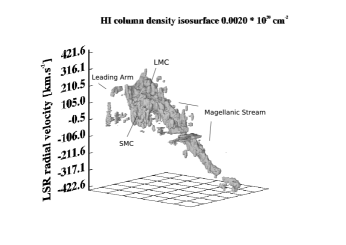
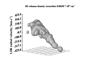
Figure 20: The figure depicts the original 3 D H I data cube by Brüns et al. (Bruens05 (2005)) (upper plot) together with the resulting data after median and Fourier filtering. Both images offer 3 D visualization of the column density isosurface $\mathrm{\Sigma_{H\,I}=0.2\cdot 10^{18}\,cm^{-2}}$.

Flexible Image Transport System (FITS) format, which lets us apply standard image processing methods naturally. A Fourier filter was selected for our task. It represents a frequency domain filter, and so it allows for an excellent control over the scale range of the image’s structures to be conserved or filtered out. We removed the wavelengths below the limit of $\mathrm{\approx 10^{\circ}}$ projected on the sky–plane. The performance of Fourier filters suffers from the presence of abrupt changes of intensity, such as edges and isolated pixels. To enhance the efficiency of frequency filtering, it was preceded by an application of a spatial median filter to smear the original image on small scales. Subsequently, the H I column density is normalized. The resulting 3 D H I column density data cube together with the original data by Brüns et al. (Bruens05 (2005)) can be seen in Fig. 20. To compare the modeled particle distribution with H I observations, we convert the distribution to a 3 D FITS image of column densities that are proportional to particle counts, since all the test–particles have the same weight factor assigned. Then, we have to interpolate missing data, which is due to a limited number of particles in our simulations. Finally, the column density is normalized to the maximal value.

After discussing the data processing and manipulation, we will introduce the individual FF components $FF_{1}$, $FF_{2}$, and $FF_{3}$.

B.1 $FF_{1}$

The observed H I LSR radial velocity profile measured along the Magellanic Stream is a notable feature of the Magellanic System. It shows a linear dependence of LSR radial velocity on Magellanic Longitude, and a high negative velocity of $\mathrm{-400\,km\,s^{-1}}$ is reached at the Magellanic Stream’s far tip (Brüns et al. Bruens05 (2005)). From the studies by Murai & Fujimoto (Murai80 (1980)) and Gardiner et al. (Gardiner94 (1994)), and from our modeling of various Magellanic evolutionary scenarios, we know that the linearity of the Magellanic Stream velocity profile shows low sensitivity to the variation of the initial conditions of the models. On the other hand, the slope of the LSR radial velocity function is a very specific feature, especially strongly dependent on the features of the orbital motion of the Clouds. Therefore, it turned out to be an efficient approach to test whether our modeled particle distribution was able to reproduce the high negative LSR redial velocity tip of the Magelanic Stream. Then, the first FF component $FF_{1}$ was defined as follows:

$$FF_{1}=\frac{1}{1+\left|\frac{\upsilon_{\mathrm{min}}^{\mathrm{obs}}-\upsilon_{\mathrm{min}}^{\mathrm{mod}}}{\upsilon_{\mathrm{min}}^{\mathrm{obs}}}\right|},$$ (12)

where $\mathrm{\upsilon_{min}^{obs}}$ and $\mathrm{\upsilon_{min}^{mod}}$ are the minima of the observed LSR radial velocity profile of the Magellanic Stream and its model, respectively.

B.2 $FF_{2}$ and $FF_{3}$

The FF components $FF_{2}$ and $FF_{3}$ compare the observed and modeled H I column density distributions in the Magellanic System for 64 separate LSR radial velocity channels of width $\Delta\upsilon=13.2\,\mathrm{km\,s^{-1}}$. For every velocity channel, H I column density values are available for ($64\cdot 128$) pixels covering the entire System. The above introduced 3 D data was obtained by modification of the original high–resolution H I data–cube by Brüns et al. (Bruens05 (2005)). Since the test–particle model is not capable of reproducing small–scale features of the explored system, filtering and reduction of resolution of the original data were necessary prior to its use for the purpose of our GA search.

The second FF component analyzes whether there is a modeled H I emission present at the positions and LSR radial velocities where it is observed. Thus, we measure the relative spatial coverage of the System observed in H I emission by the modeled matter distribution for every LSR radial velocity channel. No attention is paid to specific H I column density values here. We only test whether both modeled and observed emission is present at the same pixel of the position–velocity space. It can be expressed as

$$FF_{2}=\frac{\sum\limits_{i=1}^{N_{\upsilon}}\sum\limits_{j=1}^{N_{y}}\sum\limits_{k=1}^{N_{x}}pix_{ijk}^{\mathrm{obs}}\cdot pix_{ijk}^{\mathrm{mod}}}{MAX\left(\sum\limits_{i=1}^{N_{\upsilon}}\sum\limits_{j=1}^{N_{y}}\sum\limits_{k=1}^{N_{x}}pix_{ijk}^{\mathrm{obs}},\sum\limits_{i=1}^{N_{\upsilon}}\sum\limits_{j=1}^{N_{y}}\sum\limits_{k=1}^{N_{y}}pix_{ijk}^{\mathrm{mod}}\right)},$$ (13)

where $pix_{ijk}^{\mathrm{obs}}\in\{0,1\}$ and $pix_{ijk}^{\mathrm{mod}}\in\{0,1\}$ indicate whether there is matter detected at the position [i, j, k] of the 3 D data on the observed and modeled Magellanic System, respectively. $N_{\upsilon}=64$ is the number of separate LSR radial velocity channels in our data. $(N_{x}\cdot N_{y})=(64\cdot 128)$ is the total number of positions on the sky–plane for which observed and modeled H I column density values are available.

This binary comparison between the observed and modeled data introduces a problem of pure noise pixels present in the observed data cube because they posses the same weight as the other data, despite their typically very low intensity. However, our treatment of the original high–resolution data by Brüns et al. (Bruens05 (2005)) involves spatial median filtering. It smears abrupt intensity changes and removes isolated pixels, which handles the problem of pure–noise data pixels naturally. The subsequent Fourier filtering decreases the data resolution significantly, and that also strongly suppresses the influence of original noise pixels.

As the last step we compare the modeled matter density distribution to the observation. To do that, both modeled and observed H I column density values are scaled relative to their maxima to introduce dimensionless quantities. Then, we get

$$FF_{3}=\frac{1}{N_{\upsilon}\cdot N_{x}\cdot N_{y}}\sum\limits_{i=1}^{N_{\upsilon}}\sum\limits_{j=1}^{N_{y}}\sum\limits_{k=1}^{N_{x}}\frac{1}{1+\left|\sigma_{ijk}^{\mathrm{obs}}-\sigma_{ijk}^{\mathrm{mod}}\right|},$$ (14)

where $\sigma_{ijk}^{\mathrm{obs}}$, $\sigma_{ijk}^{\mathrm{mod}}$ are normalized column densities measured at the position [j, k] of the i–th velocity channel of the observed and modeled data, respectively.