Fast cosmological parameter estimation using neural networks

Abstract

We present a method for accelerating the calculation of CMB power spectra, matter power spectra and likelihood functions for use in cosmological parameter estimation. The algorithm, called CosmoNet, is based on training a multilayer perceptron neural network and shares all the advantages of the recently released Pico algorithm of Fendt & Wandelt, but has several additional benefits in terms of simplicity, computational speed, memory requirements and ease of training. We demonstrate the capabilities of CosmoNet by computing CMB power spectra over a box in the parameter space of flat $\Lambda$CDM models containing the $3\sigma$ WMAP1 confidence region. We also use CosmoNet to compute the WMAP3 likelihood for flat $\Lambda$CDM models and show that marginalised posteriors on parameters derived are very similar to those obtained using CAMB and the WMAP3 code. We find that the average error in the power spectra is typically $2-3\%$ of cosmic variance, and that CosmoNet is $\sim 7\times 10^{4}$ faster than CAMB (for flat models) and $\sim 6\times 10^{6}$ times faster than the official WMAP3 likelihood code. CosmoNet and an interface to CosmoMC are publically available at www.mrao.cam.ac.uk/software/cosmonet.

1 Introduction

In the analysis of increasingly high-precision data sets, it is now common practice in cosmology to constrain cosmological parameters using sampling based methods, most notably Markov chain Monte Carlo (MCMC) techniques (Christensen et al. 2001; Knox, Christensen & Skordis 2001; Lewis & Bridle 2002). This approach typically requires one to calculate theoretical CMB power spectra (i.e. some subset of the TT, TE, EE and BB $C_{\ell}$ spectra) and/or the matter power spectrum $P(k)$ at a large number of points (typically $\sim 10^{5}$ or more) in the cosmological parameter space. In addition, one must also evaluate at each point the corresponding (combined) likelihood function for the data set(s) under consideration. As a result, the process can be computational very demanding.

The purist would calculate the required power spectra at each point using codes such as CMBfast (Seljak & Zaldarriaga 1996) or CAMB (Lewis, Challinor & Lasenby 2000), which typically require around 10 secs for spatially-flat models and 50 secs for non-flat models. This approach is therefore computationally demanding, but does have the advantage that it is simple to generalise if one wishes to include new physics or change the form of the initial power spectra. MCMC parameter estimation codes such as CosmoMC (Lewis & Bridle 2002) attempt to decrease the overall computational burden by dividing the cosmological parameter space into ‘fast’ parameters (governing the initial primoridal power spectra of scalar and tensor perturbations) and ‘slow’ parameters (governing the perturbation evolution) and making judicious proposals for how the chain is propagated in parameter space. Even with this technique, however, the total computational cost is still usually very high.

If one is willing to forego the full calculation of the required power spectra at each point in parameter space, there are a number of ways in which suitably accurate spectra can be generated somewhat more rapidly. If the cosmological parameter space of interest is sufficiently small, then it is possible simply to create spectra for a regular grid of models in parameter space and interpolate between them in some way. As the number of parameters increases, however, the computational cost of constructing the grid grows exponentially. Fast grid generation schemes have been proposed, such as the $\ell$-splitting scheme of Tegmark & Zaldarriaga (2000) that exploits analytic approximations at high-$\ell$ and insensitivity to certain parameters at low-$\ell$. Nevertheless, the pre-compute of the grid of models remains extremely time-consuming and such approaches become difficult to implement accurately when second-order effects such as gravitational lensing are important.

More extensive use of analytic and semi-analytic approximations can reduce the required number of pre-computed models, but only at the cost of a loss of accuracy and/or placing restrictions on the parameters that are available as input. Such approaches are usually based on a relatively sparse grid of base models in the parameter space from which the spectra of more general models are computed rapidly on-the-fly using various (semi-)analytic approximations. The DASh code of Kaplinghat, Knox & Skordis (2002), instead stores a sparse grid of transfer functions (rather than $C_{\ell}$), uses efficient choices for grid parameters and makes considerable use of analytic approximations. Following $\sim 40$ hrs of computation on a typical desktop to calculate the grid, DASh provides a speed-up factor of $\sim 30$ relative to CMBfast in calculating a $C^{\rm TT}_{\ell}$, $C^{\rm TE}_{\ell}$ or $C^{\rm EE}_{\ell}$ spectrum. More recently, the need to pre-compute a grid of models has been removed in the CMBwarp package (Jimenez et al. 2004), which builds on the method introduced by Kosowsky, Milosavljevic & Jimenez (2002). In this approach, a new set of nearly uncorrelated ‘physical parameters’ are introduced upon which the CMB power spectra have a simple dependence. CMBwarp uses a modified polynomial fit in these parameters in which the coefficients are based on the spectra $C^{\rm TT}_{\ell}$, $C^{\rm TE}_{\ell}$ or $C^{\rm EE}_{\ell}$ for just a single fiducial model in the parameter space. Spectra for other models can then be calculated around $\sim 3000$ times faster than CMBfast. By taking the fiducial model to be the best-fit model to the WMAP1 data, CMBwarp gives better than 0.5 per cent accuracy for the $C^{\rm TT}_{\ell}$ spectrum throughout the entire region of parameter space lying within the WMAP1 3$\sigma$ confidence region, although the accuracy quickly reduces as one moves further away from the fiducial model.

Although the above methods have proved extremely useful in performing cosmological parameter estimation, they do exhibit a number of drawbacks, as we have outlined. Most recently, this has led Fendt & Wandelt (2006) to propose a more flexible and robust machine-learning approach (called Pico) to accelerating both power spectra and likelihood evaluations. In this method, one first calculates the required spectra (usually $C^{\rm TT}_{\ell}$, $C^{\rm TE}_{\ell}$ or $C^{\rm EE}_{\ell}$) using CAMB and the corresponding likelihoods for the experiments of interest (in particular WMAP3) at $\sim 10^{4}$ points chosen uniformly within a box in parameter space that encompasses (say) the $3\sigma$ confidence region of the WMAP3 likelihood. This constitutes the training set for the Pico code – note that only power spectra values at the limited number of $\ell$-values output by CAMB are used (typically $50$ values for $\ell_{\rm max}=1500$). In short, the basic algorithm used by Pico consists of three major parts. First, the training set is compressed using Karhunen–Loève eigenmodes (essentially a principal component analysis) which typically results in a reduction in the dimensionality of the training set by a factor of two. Second, the training set is used to divide the parameter space into ($\sim 100$) smaller regions using a $k$-means clustering algorithm (see e.g. MacKay 1997) with the goal that all clusters encompass volume of parameter space over which the power spectra vary roughly equally. Finally, a (4th order) polynomial is fitted within each cluster (by minimising the squared error) to provide a local interpolation of the power spectra within the cluster as a function of cosmological parameters. The reason for dividing up the parameter space in the second step is that the interpolation method used fails to model accurately the power spectra over the entire parameter space.

The Pico approach provides about the same speed-up in spectrum calculation as CMBWarp (which is an order of magnitude faster than DASh), but is an order of magnitude more accurate. It also has several other important advantages. First, it is very flexible and can easily be applied to the fast calculation of any observables relevant to a particular data set, such as scalar, tensor and lensed power spectra, transfer functions or even higher-order correlation functions. Second, it allows the calculation of such observables from an arbitrary number of cosmological models and in any range of $\ell$ (or $k$) values. Lastly, the algorithm is sufficiently generic to allow the direct fitting of likelihood functions, thereby incorporating the functionality of the CMBfit code of Sandvik et al. This last capability allows an additional order of magnitude speed-up in cosmological parameter estimation beyond that resulting from faster power spectrum calculations, and is particularly important for experiments such as WMAP3 for which the likelihood calculation is very expensive.

In this letter, we present an independent approach to using machine-learning techniques for accelerating both power spectra and likelihood evaluations. Our approach is based on training a neural network in the form of a 3-layer perceptron. The resulting CosmoNet code shares all the advantages of Pico, but we believe also has some additional benefits in terms of simplicity, computational speed, accuracy, memory requirements and ease of training. The letter is organised as follows. In Section 2 we give a brief introduction to neural networks and our training algorithm. The resulting network output is discussed in Section 3, where we investigate the accuracy of our approach. The CosmoNet code is then used to perform a cosmological parameter estimation from WMAP3 data in Section 4. Our conclusions are presented in Section 5.

2 Neural network interpolation

Neural networks are a methodology for computing motivated by the parallel architecture of animal brains. They consist of a group of interconnected processing elements called neurons that pass simple scalar messages between them to process information. Many neural networks provide feed-forward maps from a set of input neurons to a set of output neurons. For an introduction to feed-forward neural networks see Bailer-Jones et al. (2001). They are often used to provide empirical models for processes that are too complicated to model from theoretical principles. An astrophysical example is presented in Vanzella et al. (2004), where photometric redshifts are predicted in the HDF-S from an ultra deep multicolour catalogue.

2.1 Multilayer perceptron networks

The perceptron (Rosenblatt 1958) is the simplest type of feed-forward neuron and maps an input vector ${\textbf{{x}}}\in\Re^{n}$ to a scalar output $f({\textbf{{x}}};{\textbf{{w}}},\theta)$ via

$$f({\textbf{{x}}};{\textbf{{w}}},\theta)=\sum_{i}w_{i}x_{i}+\theta,$$ (1)

where $\{w_{i}\}$ and $\theta$ are the parameters of the perceptron, called the ‘weights’ and ‘bias’ respectively.

Multilayer perceptron neural networks (MLPs) are a type of feed-forward network composed of a number of ordered layers of perceptron neurons that pass scalar messages from one layer to the next. In the simplest case, the network has two layers: the input layer and and the output layer. Each node in the output layer is a perceptron and has an activation given by (1). In this paper, however, we will work with a 3-layer network, which consists of an input layer, a hidden layer and an output layer, as illustrated in Fig. 1.

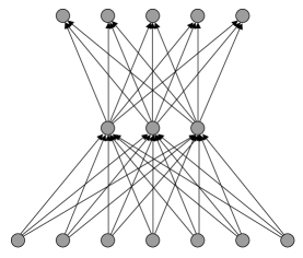
Figure 1: An example of a 3-layer neural network with seven input nodes, 3 nodes in the hidden layer and five output nodes. Each line represents one weight.

In such a network, the outputs of the nodes in the hidden and output layers take the form

hidden layer: $$h_{j}=g^{(1)}(f_{j}^{(1)}); f_{j}^{(1)}=\sum_{l}w^{(1)}_{jl}x_{l}+\theta_{j}^{(1)},$$ (2)

output layer: $$y_{i}=g^{(2)}(f_{i}^{(2)}); f_{i}^{(2)}=\sum_{j}w^{(2)}_{ij}h_{j}+\theta_{i}^{(2)},$$ (3)

where the index $l$ runs over input nodes, $j$ runs over hidden nodes and $i$ runs over output nodes. The functions $g^{(1)}$ and $g^{(2)}$ are called activation functions and are chosen to be bounded, smooth and monotonic. In this letter, we use $g^{(1)}(x)=\tanh x$ and $g^{(2)}(x)=x$, where the non-linear nature of the former is a key ingredient in constructing a viable network.

The weights w and biases $\mn@boldsymbol{\theta}$ are the quantities we wish to determine, which we denote collectively by a. As these parameters vary a very wide range of non-linear mappings between the inputs and outputs are possible. In fact, according to a ‘universal approximation theorem’ (Leshno et al. 1993), a standard multilayer feed-forward network with a locally bounded piecewise continuous activation function can approximate any continuous function to any degree of accuracy if (and only if) the network’s activation function is not a polynomial. This result applies when activation functions are chosen apriori and held fixed as a varies. Accuracy increase with the number in the hidden layer and the above theorem tells us we can always choose sufficient hidden nodes to produce any accuracy. Since the mapping from cosmological parameter space to the space of CMB power spectra (and WMAP3 likelihood) is known to be continuous, a 3-layer MLP with an appropriate choice of activation function is an excellent candidate model for the replacement of the forward model provided by the CAMB package (and WMAP3 likelihood code).

The activation functions act as basic building blocks of non-linearity in a neural network model and should be as simple as possible. Additionally, the MemSys routines used in training (described below) require derivative information and so they should be differentiable. The universal approximation theorem thus motivates us to choose a monotonic (for simplicity), bounded and differentiable function that is not a polynomial and we choose the $tanh$ function. Of course, this could be replaced by another such function, such as the sigmoid function, but the interpolation results will be almost identical.

2.2 Network training

Let us consider building an empirical model of the CAMB mapping using a 3-layer MLP as described above (a model of the WMAP3 likelihood code can be constructed in an analogous manner). The number of nodes in the input layer will correspond to the number of cosmological parameters, and the number in the output layer will be the number of uninterpolated $C_{\ell}$ values output by CAMB. A set of training data ${\cal{D}}=\{{\textbf{{x}}}^{(k)},{\textbf{{t}}}^{(k)}\}$ is provided by CAMB (the precise form of which is described later) and the problem now reduces to choosing the appropriate weights and biases of the neural network that best fit this training data.

As the CAMB mapping is exact, this is a deterministic problem, not a probabilistic one. We therefore wish to choose network parameters a that minimise the ‘error’ term $\chi^{2}({\textbf{{a}}}))$ on the training set given by

$$\chi^{2}({\textbf{{a}}})={\textstyle\frac{1}{2}}\sum_{k}\sum_{i}\left[t^{(k)}_{i}-y_{i}({\textbf{{x}}}^{(k)};{\textbf{{a}}})\right]^{2}.$$ (4)

This is, however, a highly non-linear, multi-modal function in many dimensions whose optimisation poses a non-trivial problem. Despite the deterministic nature of the problem we use an extension of a Bayesian method provided by the MemSys package (Gull & Skilling 1999).

The MemSys algorithm considers the parameters a of the network to be probabilistic variables with prior probability distribution proportional to $\exp(-\alpha S({\textbf{{a}}}))$, where $S({\textbf{{a}}})$ is the positive-negative entropy functional (Gull & Skilling 1999; Hobson & Lasenby 1998) and $\alpha$ is considered a hyperparameter of the prior. The variable $\alpha$ sets the scale over which variations in a are expected, and is chosen to maximise its marginal posterior probability. Its value is inversely proportional to the standard deviation of the prior. For fixed $\alpha$, the log-posterior is thus proportional to $-\chi^{2}({\textbf{{a}}})+\alpha S({\textbf{{a}}})$. For each choice of $\alpha$ there is a solution $\hat{{\textbf{{a}}}}$ that maximises the posterior. As $\alpha$ varies, the set of solutions $\hat{{\textbf{{a}}}}$ is called the ‘maximum-entropy trajectory’. We wish to find the maximum of $-\chi^{2}$ which is the solution at the end of the trajectory where $\alpha=0$. It is difficult to recover results for $\alpha\neq\infty$ (for large $\alpha$ the solution is found at the maximum of the prior) when starting with a result that lies far from the trajectory. Thus for practical purposes, it is best to start from the point on the trajectory at $\alpha=\infty$ and iterate $\alpha$ downwards until either a Bayesian $\alpha$ is acheived, or in our deterministic case, $\alpha$ is sufficiently small that the posterior is dominated by $\chi^{2}$.

MemSys performs the algorithm using conjugate gradients at each step to converge to the maximum-entropy trajectory. The required matrix of second derivatives of $\chi^{2}$ is approximated using vector routines only. This avoids the need for the $O(N^{3})$ operations required to perform exact calculations, that would be impractical for large problems. The application of MemSys to the problem of network training allows for the fast efficient training of relatively large network structures on large data sets that would otherwise be difficult to perform in a useful time-frame. The MemSys algorithms are described in greater detail in (Gull & Skilling 1999).

3 Results

We demonstrate our approach by training networks to replace the CAMB package for the evaluation of the CMB power spectra $C^{\rm TT}_{\ell}$, $C^{\rm TE}_{\ell}$ or $C^{\rm EE}_{\ell}$ for flat $\Lambda$CDM models within a box in parameter space that encompasses the $3\sigma$ confidence region of the WMAP 1-year likelihood. We also train a network to replace the WMAP 3-year likelihood code, however for reasons to be discussed later in this section, this interpolation was preformed over a slightly smaller region than $3\sigma$. We train four seperate networks: one for each CMB power spectra and one for the WMAP 3-year likelihood. It is possible to provide all spectra and the likelihood from a single network, but training speed is increased by keeping them separate.

The training data for the spectra interpolation is produced in a similar way to that used to train the Pico algorithm. We define the same box as Fendt & Wandelt in the 6-dimensional ‘physical parameter’ space of flat $\Lambda$CDM models, which encompasses the $3\sigma$ confidence region of the likelihood determined from WMAP 1-year data (Bennett et al. 2003) and other higher resolution CMB data. This box is then sampled uniformly to select $2000$ models. The physical parameters ($\omega_{\rm b}$, $\omega_{\rm cdm}$, $\theta$, $\tau$, $n_{\rm s}$, $A_{\rm s}$) are converted back to cosmological parameters ($\Omega_{\rm b}$, $\Omega_{\rm cdm}$, $H_{0}$, $z_{\rm re}$, $n_{\rm s}$, $A_{\rm s}$) and used as input to CAMB to produce the training set of CMB power spectra out to $\ell_{\rm max}=1500$ (which corresponds to 50 uninterpolated $C_{\ell}$ values for each spectrum). A further set of $10^{4}$ samples were generated as testing data.

Building a training set for the likelihood was complicated by errors in the WMAP 3-year likelihood code. Spuriously high likelihoods were observed for some models lying outside of roughly $2\sigma$. These spikes in the likelihood surface prevented a reasonable interpolation in these areas and so had to be eliminated from the training set. In addition sampling uniformly from a $3\sigma$ region in 6 dimensions returned very few samples around the maximum likelihood point –making an accurate interpolation around the peak unworkable. To correct for both of these problems we built our likelihood training set from $5000$ samples in parameter space drawn from a Gaussian distribution centered on the maximum likelihood point (restricted to the box encompassing our parameter priors). The covariance matrix of the Gaussian was twice that of the expected variance of the cosmological parameters and was found to provide sufficient coverage, both for the peaks of the marginalised posteriors and their tails.

A small pre-processing step was used to make the variation in the training data of a similar order to the non-linearity present in the network activation functions. This involved mapping all inputs and outputs linearly so they had zero mean and a variance of one-half. Appropriate scaling of the data would be performed by network training if this step were omitted, but the speed of training is increased if the initial values of the weights are closer to their likely optimal values. Also, for the TE and EE spectra, a small number (2-4) of separate neural networks were trained on separate regions of the spectra, and then combined post training to provide a single network for each spectra. This step was required to provide $99^{\hbox{th}}$ percentile error within those produced by the Pico algorithm.

It was found that 50 nodes in the hidden layer for the TT spectra network, 125 nodes for the TE spectra network, 200 nodes for the EE spectra network, and 50 for the likelihood network, were sufficient to provide good results. The results of comparing the CosmoNet output with CAMB over the testing set are shown in Fig. 2.

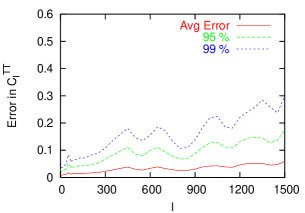
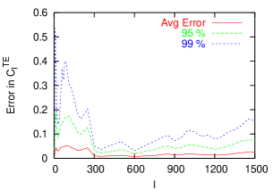
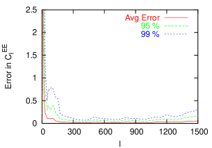
Figure 2: Comparison of the performance of CosmoNet versus CAMB for TT, TE and EE power spectra in 6-parameter flat $\Lambda$CDM models. The plots shows the average error together with the 95 and 99 percentiles in units of cosmic variance.

For all but the very low values of $l$ in the EE spectrum, where the values of the spectrum and cosmic variance are small, the average error is about $2-3\%$ of cosmic variance. The $99^{\hbox{th}}$ percentiles are also comfortably below unit cosmic variance. A comparison of output of the CosmoNet likelihood network with the WMAP3 likelihood code over the testing set reveals a mean error of roughly 0.2 $\ln$ units close to the peak.

4 Application to cosmological parameter estimation

To illustrate the usefulness of CosmoNet in cosmological parameter estimation we perform an analysis of the WMAP 3-year TT, TE and EE data using CosmoMC in three separate ways: (i) using CAMB power spectra and the WMAP3 likelihood code; (ii) using CosmoNet power spectra and the WMAP3 likelihood code; and (iii) using the CosmoNet likelihood. The resulting marginalised parameter constraints for each method are shown in Fig. 3 and Fig. 4, and are clearly very similar.

In each case 4 parallel MCMC chains were run on Intel Itanium 2 processors at the COSMOS cluster (SGI Altix 3700) at DAMTP, Cambridge. The wall-clock computational time required to gather $\sim 20000$ post burn-in MCMC samples was $\sim 12$ hours for method (i) (with CAMB further parallelised over 3 additional processors per chain, therefore totalling 16 CPUs),  8 hours for method (ii) and roughly 35$\pm 5$ minutes using the interpolated likelihood with method (iii). For comparison, a similar run with the Pico code took roughly 55$\pm 5$ minutes illustrating that it is now the remaining sampling calls within Cosmomc that provides the new bottleneck.

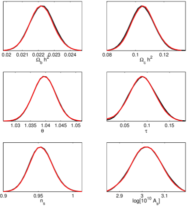
Figure 3: The one-dimensional marginalised posteriors on the cosmological parameters within the 6-parameter flat $\Lambda$CDM model comparing: CAMB power-spectra and WMAP3 likelihood (red) with CosmoNet power spectra and WMAP3 likelihood (black).

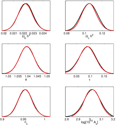
Figure 4: The one-dimensional marginalised posteriors on the cosmological parameters within the 6-parameter flat $\Lambda$CDM model comparing: CAMB power-spectra and WMAP3 likelihood (red) with CosmoNet likelihoods (black).

5 Discussion and conclusions

We have presented a method for accelerating power spectrum and likelihood evaluations based on the training of multilayer perceptron neural networks, which we have shown to be fast, robust and accurate. Our CosmoNet method shares all the advantages of the Pico algorithm of Fendt & Wandelt, achieving similar accuracies on both spectra interpolations and cosmological parameter constraints, but there are several differences between the two methods that we believe give CosmoNet a number of additional benefits, which we now discuss.

Simplicity. Despite requiring the optimisation of a highly non-linear multi-dimensional function using MemSys, we consider the principal advantage of our method to be the relative simplicity of the trained interpolation for the user to implement. CosmoNet provides a single simple, closed-form function for each interpolation over the whole of the parameter space under consideration.

Memory usage. A neural network with $N_{\rm in}$ inputs, $N_{\rm hid}$ nodes in the hidden layer, and $N_{\rm out}$ outputs has $(N_{\rm in}+1)N_{\rm hid}+(N_{\rm hid}+1)N_{\rm out}\approx N_{\rm hid}N_{\rm out}$ parameters. This is far less than in the Pico approach, where the use of clustering and individual interpolations for each $C_{\ell}$ requires far more parameters. In the case of the flat $\Lambda$CDM example demonstrated in section 3, we require about $100$ kB of parameter memory for all three power spectra and the likelihood, whereas Pico would require $15$ MB. While the memory requirements of Pico will increase with the number of cosmological parameters, this should make little difference to the memory requirements of our method, as we have found the required number of nodes in the hidden layer does not increase beyond a factor of 2 for the 11 parameter non-flat model parameterised by $\Omega_{b}h^{2}$, $\Omega_{c}h^{2}$, $\Omega_{k}$, $\theta$, $\tau$, massive neutrino fraction $f_{\nu}$, varying equation of state of dark energy $w$, scalar perturbation amplitude and spectral index $A_{s}$, $n_{s}$ and tensor modes with amplitude ratio and spectral index $R$, $n_{t}$ (results to appear in a forthcoming paper), thus representing a linear rise.

Speed. The number of calculations required to perform the feed-forward network mapping is $2N_{\rm in}\ N_{\rm hid}\ +\ 2N_{\rm hid}\ N_{\rm out}\approx 2N_{\rm hid}N_{\rm out}\$. In the example presented in section 3 the calculation of the 50 uninterpolated $C_{\ell}$ values for each spectrum required $\sim$ 120 microseconds, whereas each WMAP3 likelihood took $\sim$ 10 microseconds; this is $\sim 25$ times faster than Pico in performing the interpolation. Moreover, the CPU requirements of the Pico interpolation scales as $(\frac{N_{\rm in}}{p})^{p}$, for Pico $p$ is 4.

Ease of training. Training using the MemSys package is almost totally automated and relatively quick. In fact the bottleneck in providing appropriate network weights for more complex cosmological models is the calculation of the training data using the CAMB package. The networks used in section 3 took around 100 hours of training (on a standard PC workstation). Additionally, MemSys training time scales linearly with the number of network nodes and again linearly with the number of entries in the training set. However, networks with an accuracy of roughly $2-3$ times worse, that are sufficient to provide good parameter constraints can be trained in under an hour using just 1000 training samples. These simpler neural networks did not require the l-splitting performed in section 3 and had only 50 nodes in the hidden layer.

ACKNOWLEDGMENTS

TA acknowledges a studentship from EPSRC. MB was supported by a Benefactors Scholarship at St. John’s College, Cambridge and an Isaac Newton studentship. This work was conducted in cooperation with SGI/Intel utilising the Altix 3700 supercomputer at DAMTP Cambridge supported by HEFCE and PPARC. We thank S. Rankin and V. Treviso for their assistance.

References

- (1) Bailer-Jones C., 2001, Automated Data Analysis in Astronomy. Narosa Publishing House, New Delhi
- (2) Bennett C. et al., 2003, ApJS, 148, 1
- (3) Christensen N., Meyer R., Knox L., Luey B., 2001, Class. Quant. Grav., 18, 2677
- (4) Fendt W., Wandelt B., 2006, ApJ, submitted (astro-ph/0606709)
- (5) Gull S.F., Skilling J., 1999, Quantified maximum entropy: MemSys 5 users’ manual. Maximum Entropy Data Consultants Ltd, Royston
- (6) Hinshaw G. et al. 2006, ApJ, submitted (astro-ph/0603451)
- (7) Hobson M.P., Lasenby A.N., 1998, MNRAS, 298, 905
- (8) Jimenez R., Verde L., Peiris H., Kosowsky A., 2004, PRD, 70, 023005
- (9) Kaplinghat M., Knox L., Skordis C., 2002, ApJ, 578, 665
- (10) Kosowsky A., Milosavljevic M., Jimenez R., 2002, PRD, 66, 063007
- (11) Knox L., Christensen N., Skordis C., 2001, ApJ, 563, L95
- (12) Lewis A., Bridle S., 2002, PRD, 66, 103511
- (13) Lewis A., Challinor A., Lasenby A., 2000, ApJ, 538, 473
- (14) Leshno M., Ya. Lin V., Pinkus A., Schocken S., 1993, Neural Netw., 1993, 6, 861
- (15) MacKay D.J.C., 2003, Information theory, inference and learning algorithms. Cambridge University Press
- (16) Page L. et al., 2006, ApJ, submitted (astro-ph/0603450)
- (17) Rosenblatt F., 1958, Psychological Review, 65, 386
- (18) Sandvik H.B., Tegmark M., Wang X., Zaldarriaga M., 2004, PRD, 69, 063005
- (19) Seljak U., Zaldarriaga M., 1996, ApJ, 469, 437
- (20) Spergel D. et al., 2006, ApJ, submitted (astro-ph/0603449)
- (21) Tegmark M., Zaldarriaga M., 2000, ApJ, 544, 30
- (22) Vanzella E. et al., 2004, A&A, 423, 761