The probability distribution of the Ly$\alpha$ transmitted flux from a sample of SDSS quasars

Abstract

We present a measurement of the probability distribution function (PDF) of the transmitted flux in the Ly$\alpha$ forest from a sample of 3492 quasars included in the SDSS DR3 data release. Our intention is to investigate the sensitivity of the Ly$\alpha$ flux PDF as measured from low resolution and low signal-to-noise data to a number of systematic errors such as uncertainties in the mean flux, continuum and noise estimate. The quasar continuum is described by the superposition of a power law and emission lines. We perform a power law continuum fitting on a spectrum-by-spectrum basis, and obtain an average continuum slope of $\alpha_{\nu}=0.59\pm 0.36$ in the redshift range $2.5<z<3.5$. Taking into account the variation in the continuum indices increases the mean flux by 3 and 7 per cent at $z=3$ and 2.4, respectively, as compared to the values inferred with a single (mean) continuum slope. We compare our measurements to the PDF obtained with mock lognormal spectra, whose statistical properties have been constrained to match the observed Ly$\alpha$ flux PDF and power spectrum of high resolution data. Using our power law continuum fitting and the SDSS pipeline noise estimate yields a poor agreement between the observed and mock PDFs. Allowing for a break in the continuum slope and, more importantly, for residual scatter in the continuum level substantially improves the agreement. A decrease of $\sim$10-15 per cent in the mean quasar continuum with a typical rms variance at the 20 per cent level can account for the data, provided that the noise excess correction is no larger than $~{}\hbox to0.0pt{$<$\hss}{\lower 4.30554pt\hbox{$\sim$}}10$ per cent.

1 Introduction

The Ly$\alpha$ forest seen in quasar spectra probes the intergalactic medium (IGM) and the underlying matter distribution over a wide range of scales ($k\sim 0.1-10\ {\rm{\it h}Mpc^{-1}}$) and redshifts ($1~{}\hbox to0.0pt{$<$\hss}{\lower 4.30554pt\hbox{$\sim$}}z~{}\hbox to0.0pt{$<$\hss}{\lower 4.30554pt\hbox{$\sim$}}6$). Measurements of the mean flux in the Ly$\alpha$ forest shed light on the reionization history and the physical state of the IGM in the post-reionization area (Press, & Rybicki & Schneider 1993, hereafter P93; Rauch et al. 1997; Bernardi et al. 2003, hereafter B03; Bolton & Haehnelt 2006). Fluctuations in the Ly$\alpha$ flux are of great interest since they provide information on the matter distribution on scales smaller than those accessible to other observables (e.g. Croft et al. 1998; 1999; 2002b; Nusser & Haehnelt 1999; 2000; Pichon et al. 2002; Zaldarriaga, Hui & Tegmark 2003; McDonald et al. 2000; McDonald et al. 2005a). Combined with CMB observations, the power spectrum of the Ly$\alpha$ forest can provide stringent constraints on the shape and amplitude of the primordial power spectrum (Seljak et al. 2004; Viel & Haehnelt 2005).

The probability distribution function (PDF) of the Ly$\alpha$ transmitted flux was first studied by Jenkins & Ostriker (1991). It has, however, received less attention in the past years as it is more sensitive to systematics errors such as continuum fitting uncertainties. Yet, the tension between the WMAP and Ly$\alpha$ values of the normalisation amplitude $\sigma_{8}$ argues in favour of incorporating statistics others than the Ly$\alpha$ flux power spectrum. Rauch et al. 1997 and McDonald et al. (2000) have computed the PDF of the Ly$\alpha$ transmitted flux from high resolution data and found that $\Lambda$CDM cosmologies provide a good fit to the observations. Gaztañaga & Croft (1999) have provided an analytic description of the Ly$\alpha$ flux PDF based on perturbation theory. Choudhury, Srianand & Padmanabhan (2001), and Desjacques & Nusser (2005) have investigated the constraints obtained from a joint fit of the PDF and power spectrum of the Ly$\alpha$ transmitted flux. Becker, Rauch & Sargent (2006) have examined the redshift evolution of the flux Ly$\alpha$ PDF from a large sample of Keck HIRES data. Note also that Lidz et al. (2005) have advocated working with the PDF of the fluctuations in the flux about the mean as it is insensitive to the quasar continuum.

The Sloan Digital Sky Survey (SDSS; York et al. 2000) has greatly increased the statistical power of the Ly$\alpha$ forest. Unfortunately, attempts to exploit the data are plagued by a number of poorly constrained parameters that describe the physical state of the IGM, by inaccuracies in the numerical modelling of the Ly$\alpha$ forest, and by systematics errors in the measurement such as continuum fitting uncertainties. The observed flux in the Ly$\alpha$ region of a quasar (QSO) spectrum depends both on the quasar continuum (the flux emitted by the quasar, including the emission lines) and on the amount of absorption by intervening galactic matter (lines and continuum absorptions). The transmitted (or normalized) flux obtained by continuum fitting of the observed spectrum is related to the optical depth along the line of sight as

$$F(w)\equiv I_{\rm obs}(w)/I_{\rm cont}={\rm e}^{-\tau(w)}\;,$$ (1)

where $\tau$ is the optical depth, $w$ is the redshift space coordinate along the line of sight, $I_{\rm obs}$ is the observed flux and $I_{\rm cont}$ is the flux emitted from the source (quasar) that would be observed in the absence of any intervening material. To estimate the unabsorbed continuum, two different approaches have been used. When the signal-to-noise is large, a polynomial continuum is fitted to regions of the Ly$\alpha$ forest free of absorption (e.g. Rauch et al. 1997; McDonald et al. 2000). When the signal-to-noise is low, one usually extrapolate the continuum redward of the Ly$\alpha$ emission line, assuming a power law shape. The last method only provides an approximation to the true continuum, and can easily introduce several types of systematic errors (e.g. Steidel & Sargent 1987). The strong degeneracy between the effective optical depth $\tau_{\rm eff}=-{\rm ln}\langle F\rangle$ and the continuum level affects the determination of the clustering amplitude $\sigma_{8}$. Measurements of the effective optical depth from low resolution quasar spectra with comparable signal-to-noise (P93; B03) are systematically higher than those based on high-resolution spectra by 10-20 per cent. As argued by Seljak et al. (2003), Tytler et al. (2004), Viel et al. (2004b), this is most likely due to systematic errors in the continuum fitting procedure of the low resolution spectra. Furthermore, the low signal-to-noise of SDSS spectra in the Ly$\alpha$ region ($S/N\sim 3$ typically) requires an accurate noise estimate. Systematic errors in the noise characterisation will affect the accuracy of the measurements. In this respect, several lines of recent evidence suggest that the SDSS reduction pipeline underestimates the true noise by 5-10 per cent (McDonald et al. 2006; Burgess 2004).

In this paper, we measure the PDF of the Ly$\alpha$ transmitted flux from a large (public) sample of quasars included in the SDSS DR3 data release (Abazajian et al. 2005). We assume that the quasar continuum follows the parametric form given in B03. However, unlike B03, we also allow for the variation in the continuum indices of individual spectra and fit a power law continuum for each spectrum separately. We compare our measurements to the probability distribution obtained from lognormal, realistic looking SDSS spectra. The statistical properties of these mock spectra are beforehand constrained to match the observed Ly$\alpha$ flux probability distribution and power spectrum of high resolution data of the forest. Our intention is to investigate the sensitivity of the Ly$\alpha$ flux PDF as measured from low resolution, low signal-to-noise data to a number of systematic errors such as uncertainties in the mean flux, continuum and noise estimate.

The paper is organised as follows. We briefly review the lognormal model of the Ly$\alpha$ forest in Section §2. The constraints on the model parameters are discussed in §3. The continuum fitting procedure and the measurement of the PDF of the Ly$\alpha$ flux are presented in §4. In §5, we compare the simulated and observed PDF, and study the effect of a number of systematic errors. We discuss our results in §6. In  §7, we conclude and indicate potential future works. We will present results for a $\Lambda$CDM cosmology with normalisation amplitude $\sigma_{8}=0.83$, and spectral index $n_{s}=0.96$. This is consistent with the constraints obtained from the latest CMB and Ly$\alpha$ forest data (Spergel et al. 2006; Viel, Haehnelt & Lewis 2006; Seljak, Slosar & McDonald 2006).

2 Generating mock quasar spectra

We implement the lognormal model introduced by Bi and collaborators (Bi, Börner & Chu 1992; Bi 1993; Bi & Davidsen 1997; see also Choudhury, Padmanabhan & Srianand 2001; Viel et al. 2002) to simulate the distribution of low-column density Ly$\alpha$ absorption lines along the LOS to quasars. The main advantage of this procedure is that simulated spectra can have an arbitrary large length. This allows us to eliminate periodicity effects that are present in simulations, where the typical box size is noticeably smaller than the total length of a single spectrum. Furthermore, this approach is computationally very efficient as compared to N-body simulations.

2.1 The lognormal model of the Ly$\alpha$ forest

The lognormal model of the IGM is based on the assumption that the low-column density Ly$\alpha$ forest is produced by mildly nonlinear fluctuations ($\delta\rho/\rho~{}\hbox to0.0pt{$<$\hss}{\lower 4.30554pt\hbox{$\sim$}}10$) which smoothly trace the dark matter distribution. The IGM density contrast $\delta_{\rm b}$ is obtained from a local mapping of the linear IGM density contrast $\delta_{\rm L}$ (Coles & Jones 1991), but the IGM peculiar velocity along the line of sight is assumed to be linear even on scales where the density contrast gets non-linear (Bi & Davidsen 1997) . We have namely

$$\delta_{\rm b}(x,z) = \exp\left(\delta_{\rm L}(x,z)-\sigma_{\rm L}^{2}(z)/2\right)-1$$

$$v_{\rm b}(x,z) = v_{\rm L}(x,z)\;,$$ (2)

where $\sigma_{\rm L}(z)$ is the rms fluctuations of the linear IGM density field at redshift $z$. The linear IGM density and peculiar velocity, $\delta_{\rm L}$ and $v_{\rm L}$, are obtained by smoothing the linear matter density and velocity distribution on some characteristic scale $x_{\rm F}=1/k_{\rm F}$ to mimic pressure smoothing. The linear IGM clustering amplitude, $\sigma_{\rm L}$, is thus

$$\sigma_{\rm L}^{2}=D(z)^{2}\int_{0}^{\infty}\!\!{\rm d}{\rm ln}k\,\Delta_{\rm L}^{2}(k)W_{\rm b}^{2}(k,k_{\rm F})\;,$$ (3)

where $D(z)$ is the linear density growth factor, $\Delta_{\rm L}^{2}(k)$ is the dimensionless, linear matter power spectrum at the present epoch (Peebles 1980) and $W_{\rm b}(k,k_{\rm F})$ is the IGM filter. We take the $k$-space filter $W_{\rm b}$ to be a Gaussian. Such a filter gives a good fit to the gas fluctuations over a wide range of wavenumber (Gnedin et al. 2003; see also Zaroubi et al. 2005). In principle, we expect $k_{\rm F}$ to depend on the physical state of the IGM. However, since the relation between $k_{\rm F}$ and $\hat{T}_{\rm g}$ depends noticeably on the reionization history of the Universe (Gnedin & Hui 1998; Nusser 2000), it is more convenient to treat $k_{\rm F}$ as a free parameter.

We calculate the Ly$\alpha$ transmitted flux $F=\exp(-\tau)$ in the fluctuating Gunn-Peterson approximation (Gunn & Peterson 1965, Bahcall & Salpeter 1965). The optical depth for Ly$\alpha$ resonant scattering at some redshift space position $\omega$ is expressed as a convolution of the real space HI density along the line of sight with a Voigt profile ${\cal H}$,

$$\tau(w)=\frac{c\sigma_{0}}{H(z)}\int_{-\infty}^{+\infty}\!\!dx\,n_{{}_{\rm HI}}(x){\cal H}\left[w-x-v_{\rm b}(x),b(x)\right]\;.$$ (4)

where $\sigma_{0}=4.45\times 10^{-18}\ {\rm cm^{-2}}$ is the effective cross-section for resonant line scattering, H$(z)$ is the Hubble constant at redshift $z$, $x$ is the real space coordinate, $n_{{}_{\rm HI}}(x)$ is the neutral hydrogen density, $b(x)$ is the Doppler parameter due to thermal/turbulent broadening and ${\cal H}(x)$ is the Voigt profile, which can be approximated by a Gaussian for moderate optical depths. The HI hydrogen density, $n_{{}_{\rm HI}}(x)$, and the Doppler parameter, $b(x)$, are computed using a tight polytropic relation (Katz et al. 1996, Hui & Gnedin 1997, Theuns et al. 1998) that produces results comparable to full hydrodynamical simulations,

$$n_{{}_{\rm HI}}(x) = {\hat{n}}_{{}_{\rm HI}}\left(1+\delta_{\rm b}\right)^{2-0.7(\gamma-1)}$$

$$b(x) = \hat{b}\left(1+\delta_{\rm b}\right)^{(\gamma-1)/2}\;,$$ (5)

where the adiabatic index $\gamma$ is in the range $1-1.6$. ${\hat{n}}_{{}_{\rm HI}}$ and $\hat{b}$ are the HI hydrogen density and Doppler parameter at mean gas density respectively. The latter is a function of the IGM temperature, $\hat{b}=13\ {\rm km\,s^{-1}}\hat{T}_{4}^{1/2}$, where $\hat{T}_{4}$ is the IGM temperature at mean density (in unit of $10^{4}\,{\rm K}$). Note that, since ${\hat{n}}_{{}_{\rm HI}}$ is usually constrained by fixing the mean flux level, $\langle F\rangle$, we will treat $\langle F\rangle$ as a free parameter in the remaining of this paper.

2.2 The simulation method

We simulate the Ly$\alpha$ transmitted flux in a periodic line of sight of comoving length $L$ at $N$ discrete $r$-space position $x_{i}$, $i=1,\cdots,N$. Following Bi (1993), we generate two fields $\delta_{\rm L}(k)$ and $v_{\rm L}(k)$ at discrete $k$-space positions. The two fields are correlated Gaussian random fields that can be written as linear combination of two independent fields $u(k)$ and $w(k)$ having (dimensionless) power spectra $\Delta_{\rm u}^{2}(k)$ and $\Delta_{\rm w}^{2}(k)$,

$$\delta_{\rm L}(k,z) = D(z)\left(u(k)+w(k)\right)$$

$$v_{\rm L}(k,z) = iqE(z)\frac{H_{0}}{c}f(k)w(k)\,,$$ (6)

where $E(z)$ is the linear growth factor of the velocity field. $\Delta_{\rm u}^{2}(k)$, $\Delta_{\rm w}^{2}(k)$ and $f(k)$ are constrained by the auto- and cross-correlations of the density and velocity fields,

$$f(k) = \int_{k}^{\infty}\!\!{\rm d}{\rm ln}q\,q^{-5}\Delta_{\rm 3D}^{2}(q)\,/\int_{k}^{\infty}\!\!{\rm d}{\rm ln}q\,q^{-3}\Delta_{\rm 3D}^{2}(q)$$

$$\Delta_{\rm w}^{2}(k) = f(k)^{-1}\,\int_{k}^{\infty}\!\!{\rm d}{\rm ln}q\,q^{-3}\Delta_{\rm 3D}^{2}(q)$$

$$\Delta_{\rm u}^{2}(k) = \Delta_{\rm 1D}^{2}(k)-\Delta_{\rm w}^{2}(k)\;,$$ (7)

where $\Delta_{\rm 3D}^{2}$ and $\Delta_{\rm 1D}^{2}$ are the 3D and 1D power spectra, respectively. We obtain the linear IGM density and peculiar velocity field in $r$-space from a fast Fourier transform (FFT), and calculate the mean transmitted flux by combining equations (2), (4) and (5). For a given cosmological model, the flux distribution depends only on the filtering wavenumber $k_{\rm F}$, the mean flux $\langle F\rangle$, the adiabatic index $\gamma$ and the mean IGM temperature $\hat{T}_{4}$.

2.3 Properties of the synthetic spectra

To create realistic mock spectra, we compute the flux distribution on a one-dimensional (1D) grid whose resolution $\Delta$ is fine enough to resolve the smallest structure on the filtering scale, and whose length $L$ is long enough to incorporate most of the fluctuation power. We typically have $\Delta~{}\hbox to0.0pt{$<$\hss}{\lower 4.30554pt\hbox{$\sim$}}0.002\ {\rm{\it h}^{-1}Mpc}$ and $L~{}\hbox to0.0pt{$>$\hss}{\lower 4.30554pt\hbox{$\sim$}}1000\ {\rm{\it h}^{-1}Mpc}$ (comoving). We constrain the mean flux level $\langle F\rangle$ from a large sample of idealised, noise-free spectra. Instrumental resolution, noise and strong absorption systems are included as described below. Note that, in low resolution spectra, $\langle F\rangle$ will generally differ from the “effective” mean flux $\bar{F}$ of the processed spectra, which include a number of strong absorption systems.

2.3.1 Instrumental noise and resolution

We attempt to include instrumental noise and resolution in our synthetic spectra in a way that mimics the observations as much as possible (e.g. Rauch et al. 1997). We smooth the spectra with a Gaussian of constant width, and re-sample them on pixels of wavelength size $\Delta\lambda$, interpolating between adjacent values in the fine grid. The spectra are not modified to include continuum fitting uncertainties as the latter are taken out from the observed spectra.

In the high resolution spectra, the transmitted flux is convolved with a Gaussian of full width at half maximum (FWHM) $6.6\ {\rm km\,s^{-1}}$, and re-sampled on pixels of wavelength size $\Delta\lambda=0.04\AA$. In units of $\ {\rm km\,s^{-1}}$, the resolution varies from $2\ {\rm km\,s^{-1}}$ at $z=3.9$ to $2.9\ {\rm km\,s^{-1}}$ at $z=2.4$. Further, Gaussian noise is added to each pixel with an amplitude given by a flux-dependent rms noise per pixel, $n(F)$, as measured in M00 (see their Table 3).

In the low resolution spectra, we adopt a FWHM of $170\ {\rm km\,s^{-1}}$ (i.e. a dispersion of $\approx 70\ {\rm km\,s^{-1}}$), and re-sample the flux on a uniform grid with $\Delta\log_{10}\lambda=10^{-4}$. The low signal-to-noise of the SDSS spectra in the Ly$\alpha$ region requires an accurate description of the noise. The true error on each pixel in each quasar spectrum is essentially made up of the Poisson noise from photon counts, the CCD read-noise and systematics errors from sky subtraction. McDonald et al. (2006) have outlined a procedure which follows closely the spectroscopic data reduction pipeline. The inconvenience of this method is that it requires a sky-flux estimate. Here, we simply assume that the noise distribution is Gaussian whose rms variance is given by the SDSS data reduction pipeline. Although the latter computes a variance for each flux pixel, there is some evidence that these error estimates do not perfectly reflect the true errors in the data (Bolton et al. 2004; McDonald et al. 2006; Burgess 2004). McDonald et al. (2006) and Burgess (2004) have recalibrated the noise of their spectra by differencing multiple exposures, and found that the rms noise variance given by the SDSS pipeline is underestimated by resp. 8 and 5 per cent on average. We will hereafter refer to $\sigma_{p}$ as the fiducial (pipeline) noise estimate. The sensitivity of the mock spectra to the noise level will be discussed in detail in §5.2. Given the relatively broad distribution of pixel noise variances at fixed flux $F$, we use the full set of rms noise variances from the data points with $0<F<1$. We then map with repetition the individual noise estimates onto the pixels $0<F<1$ in the idealized mock spectra (e.g. Burgess 2004). Our mapping accounts for the fact that the mean pixel noise increases with redshift (see Figure 3).

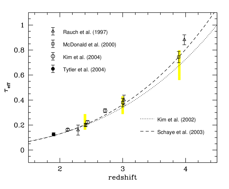
Figure 1: The effective optical depth $\tau_{\rm eff}=-{\rm ln}\langle F\rangle$ as measured from high-resolution spectra. The empty triangles, squares and circles show the measurements of Rauch et al. (1997), McDonald et al. (2000) and Kim et al. (2004). The filled circle is the measurement of Tytler et al. (2004). The dotted and dashed curves show the evolution reported by Kim et al. (2002) and Schaye et al. (2003). The vertical extent of the shaded regions indicate the values considered in our analysis.

2.3.2 Strong absorption systems

High column density systems associated with collapsed objects such as disk galaxies are not reproduced in the lognormal model (Bi & Davidsen 1997). Large column densities are needed ($N_{{}_{\rm HI}}~{}\hbox to0.0pt{$>$\hss}{\lower 4.30554pt\hbox{$\sim$}}10^{17}\ {\rm cm^{-2}}$) to produce the strong damping wings of the observed absorption line profile. In the high-resolution data, damped Ly$\alpha$ systems (DLAs) are removed by eliminating wavelength intervals containing these absorption lines from the spectra. These strong absorption lines are, however, present in our sample of SDSS spectra. We, therefore, include a set of DLAs and Lyman limit systems (LSS) in the low resolution mock spectra. We follow the procedure outlined in McDonald et al. (2005b), which is based on the self-shielding model of Zheng & Miralda-Escudé (2002). The column density distribution of these strong absorbers is then normalised to reproduce the observations of Peroux et al. 2003 and Prochaska, Herbert-Fort & Wolfe (2005). As the Doppler parameter distribution of the strong absorption systems is largely unknown, we use a single value of 30$\ {\rm km\,s^{-1}}$ at all redshifts.

3 Constraining the model parameters from high resolution data

In this Section, we constrain the model parameters from a comparison between the flux power spectrum (PS) and probability distribution (PDF) of the transmitted flux of mock and observed high resolution spectra. Desjacques & Nusser (2005) have pointed out that models that match best the PS alone do not necessarily yield a good fit to the PDF. It is therefore important to combine the PS and PDF statistics to ensure that both are correctly reproduced in the lognormal spectra. We perform a $\chi^{2}$ statistical test for the observed flux power spectrum and PDF to determine quantitatively the values of the parameter required to fit high resolution measurements of the Ly$\alpha$ forest.

3.1 The high resolution data

We use the measurements of McDonald et al. (2000), which were obtained from a sample of eight high resolution QSO spectra. Results are provided for three redshift bins centered at $z=2.41$, $3.00$ and $3.89$. Regarding the flux power spectrum, we consider the data points in the range $0.005<k<0.05\ {\rm s\,km^{-1}}$. The lower limit $k=0.005\ {\rm s\,km^{-1}}$ is chosen so as to avoid continuum fitting errors (Hui et al. 2001), and the upper limit $k=0.05\ {\rm s\,km^{-1}}$ is chosen to avoid metal contamination on smaller scales (Kim et al. 2004). The observed flux PDF is very sensitive to continuum fitting, especially in the high transmissivity tail (e.g. Meiksin, Bryan & Machacek 2001). The modelling of these errors is complicated by the fact that the scales of interest are of the order of the box size $L$ of the simulations. However, M00 demonstrate that, if the inclusion of continuum fitting errors can account for most of the discrepancy between the simulated and observed PDF in the range $F~{}\hbox to0.0pt{$>$\hss}{\lower 4.30554pt\hbox{$\sim$}}0.8$, it should not greatly affect the PDF for $F~{}\hbox to0.0pt{$<$\hss}{\lower 4.30554pt\hbox{$\sim$}}0.8$. We, therefore, exclude the data points with $F\geq 0.8$ from the analysis to avoid dealing with those errors. The M00 measurements are shown in Figure 2 as the filled symbols. The shaded areas indicate the data points used in this analysis is (10+15=25 measurements from the PS and PDF respectively).

3.2 The parameter grid

For each value of the parameter vector ${\bf p}$=($k_{\rm F}$,$\langle F\rangle$,$\gamma$,$\hat{T}_{4}$), we generate mock catalogues of 1000 lines of sight. We let the filtering wavenumber, the IGM adiabatic index and temperature assume the following values,

$$k_{\rm F} = 5.55,6.25,7.14,8.33,10,12.5,16.67,25,50$$

$$\gamma = 1,1.2,1.4,1.6$$

$$\hat{T}_{4} = 1,1.5,2,2.5,$$

irrespective of the redshift. The values of $k_{\rm F}$ (in unit of $\ {\rm{\it h}Mpc^{-1}}$) are chosen such that $1/k_{\rm F}$ uniformly spans the range $0.02-0.18\ {\rm{\it h}^{-1}Mpc}$.

The assumed effective optical depth $\tau_{\rm eff}$ or, equivalently, mean flux $\langle F\rangle=\exp(-\tau_{\rm eff})$ has a large impact on the simulated one- and two-point statistics of the forest. Observations indicate that $\tau_{\rm eff}$ evolves strongly in the redshift range $2~{}\hbox to0.0pt{$<$\hss}{\lower 4.30554pt\hbox{$\sim$}}z~{}\hbox to0.0pt{$<$\hss}{\lower 4.30554pt\hbox{$\sim$}}4$. In Fig.1, we show several measurements of $\tau_{\rm eff}$ obtained from high resolution observations. Empty triangles, squares and circles show the results of Rauch et al. (1997) and McDonald et al. (2000) for a comparable sample of HIRES spectra, whereas the empty circles indicate the estimates of the LUQAS sample of Kim et al. (2004). The filled circle shows the measurements of Tytler et al. (2004). The dotted and dashed curves indicate the evolution reported by Kim et al. (2002) and Schaye et al. (2003). Note that there is significant overlap among the quasar samples of Schaye et al. (2003) and Kim et al. (2004). All these estimates have been obtained after removing damped/sub-damped Ly$\alpha$ systems and pixels contaminated by associated metal absorption. The measurements of $\tau_{\rm eff}$ are mostly affected by cosmic variance due to large variations between lines of sight, uncertainties in the continuum fitting procedure and the somewhat uncertain contribution from metal lines (P93; Zuo & Bond 1994; Rauch et al. 1997; Tytler et al. 2004; Viel et al. 2004a). In particular, the continuum fitting generally adopted for high resolution data may result in an underestimation of the continuum and of $\tau_{\rm eff}$ (Kim et al. 2001). Based on these measurements, we adopt the following values for the mean flux $\langle F\rangle$ : $0.45\leq\langle F\rangle\leq 0.55$ ($z=2.4$), $0.65\leq\langle F\rangle\leq 0.75$ ($z=3$) and $0.75\leq\langle F\rangle\leq 0.85$ ($z=3.9$). These intervals are shown as shaded regions in Fig. 1. Although the effective optical depth appears to evolve smoothly with redshift, the behaviour of $\tau_{\rm eff}(z)$ inferred from a large sample of SDSS quasars is found to deviate from a power law around $z=3.2$ (B03), suggesting that HeII reionizes in that redshift range (Theuns et al. 2002b; Schaye et al. 2000).

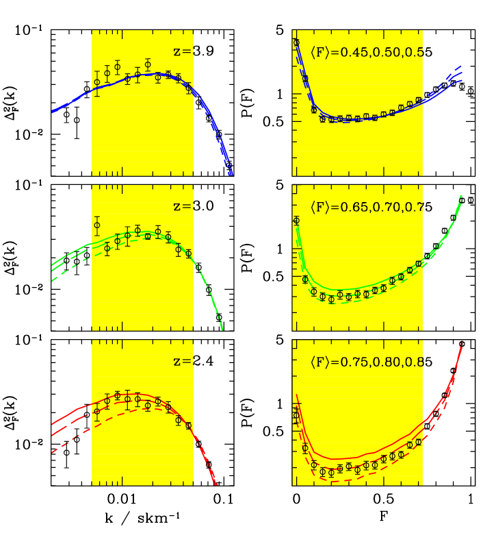
Figure 2: The flux power spectrum and PDF of the best-fitting models ($\Delta\chi^{2}=0$) at redshift $z=3.9$ (top), 3.0 (middle) and 2.4 (bottom). The mean flux is, respectively, $\langle F\rangle=0.45$, 0.5, 0.55, $\langle F\rangle=0.65$, 0.7, 0.75, and $\langle F\rangle=0.75$, 0.8, 0.85. In each panel, the solid and short-dashed curves stand for the lowest and largest values of $\langle F\rangle$, respectively. The IGM temperature has a fixed value, $\hat{T}_{4}=1.5$. Only $k_{\rm F}$ and $\gamma$ are varied to obtain the best-fitting parameters. The shaded regions indicate the data points we use to compute the value of $\chi^{2}$. The best-fitting values of $k_{\rm F}$ and $\gamma$, together with the chi-squared value are listed in Table  1.

We use a spectral grid of $N=2^{19}$ pixels which are evenly spaced in wavelength ($\Delta\lambda=0.005\AA$). $N$ and $\Delta$ are chosen so that the number of pixels in the “degraded” mock spectra is a constant power of 2 to facilitate the computation of Fourier transforms.

For each mock catalogue, we calculate the flux power spectrum and the flux PDF. We determine the goodness of fit of any model in the grid by computing a $\chi^{2}$ statistic from the difference between the simulated PS and PDF and the observational data. In the calculation of the $\chi^{2}$, we neglect the correlations between measurements of the flux PS. However, in the case of the flux PDF, we include the full covariance matrix since these measuremements are highly correlated (M00). We take advantage of the smooth dependence of the flux PS and PDF on the parameter vector, and use cubic spline interpolation to find the best-fitting models.

Table 1: Parameter values of the models which best fit the PS and PDF inferred from high-resolution measurements of the Ly$\alpha$ forest. The mean IGM temperature has a fixed value $\hat{T}_{4}=1.5$. Only $k_{\rm F}$ and $\gamma$ are varied to obtain the best-fitting models. The filtering $k_{\rm F}$ is in unit of $\ {\rm{\it h}Mpc^{-1}}$. The last column gives the chi-squared for 23 degrees of freedom. Note that, since we spline interpolate over the parameters, the best fit values do not necessarily lie at a grid point.

redshift	$\langle F\rangle$	$k_{\rm F}$	$\gamma$	$\chi^{2}$
3.9	0.45	37.1	1.00	24.6
	0.50	32.7	1.00	26.7
	0.55	36.3	1.12	45.7
3.0	0.65	18.3	1.00	39.5
	0.70	20.5	1.00	22.6
	0.75	32.8	1.16	40.7
2.4	0.75	12.5	1.00	108.8
	0.80	15.5	1.00	41.8
	0.85	25.0	1.00	46.3

3.3 The best-fitting models

Fig. 2 compares the best-fitting models to the M00 data at redshift $z=3.9$ (top panels), 3.0 (middle panels) and 2.4 (bottom panels). The parameter values of the models are listed in Table 1. The solid, long dashed and short dashed curves show, respectively, the models with lowest, intermediate and largest value of $\langle F\rangle$ at a given redshift. The IGM temperature has a fixed value, $\hat{T}_{4}=1.5$. Only $k_{\rm F}$ and $\gamma$ are varied to obtain the best-fitting parameters. The shaded regions indicate the data points we use to compute the value of $\chi^{2}$. Note that the 1D grid resolves the best-fitting values of the filtering length with 10 cells at least. The best-fitting models provide an acceptable fit to the data down to redshift $z=3$. At $z=3.9$ and 3, the best chi-squared has an acceptable value of $\chi^{2}~{}\hbox to0.0pt{$<$\hss}{\lower 4.30554pt\hbox{$\sim$}}25$ for 23 degrees of freedom (25 data points minus the filtering length and adiabatic index). At $z=2.4$ however, $\chi^{2}~{}\hbox to0.0pt{$>$\hss}{\lower 4.30554pt\hbox{$\sim$}}40$, which should be exceeded randomly only $\sim$1.5 per cent of the time. As expected, the lognormal approximation no longer provides a good fit (in a chi-squared sense at least) to the data for $z<3$ (e.g. Nusser & Haehnelt 2000). For most of the models, the best-fitting value of the adiabatic index is $\gamma=1$, whereas observations indicate that $\gamma\sim 1.3-1.5$ in the redshift range considered here (Schaye et al. 2000b; McDonald & Miralda-Escudé 2001). Note, however, that there is a degeneracy between the filtering wavenumber $k_{\rm F}$ and the adiabatic index $\gamma$ which allows one to match the data with larger values of $\gamma$ and $k_{\rm F}$ (Desjacques & Nusser 2005; see also Meiksin & White 2001).

The M00 results are averaged in relatively large redshift bins, $2.09\leq z\leq 2.67$, $2.67\leq z\leq 3.39$ and $3.39\leq z\leq 4.43$. The evolution of the mean flux $\langle F\rangle$, for example, is significant over those redshift intervals. We could account for the redshift evolution by averaging mock catalogues computed at different $z$ in the same redshift bin before comparing with the observations. However, this correction is difficult to apply as the exact dependence of $k_{\rm F}$, $\gamma$ and $\hat{T}_{4}$ on the redshift is unknown. Additional assumptions on the reionization history of the Universe could reduce the freedom in the parameter space. In this respect, the observed line-width distribution suggests that, around $z=3$, there is a sharp increase in $\hat{T}_{\rm g}$ together with a decrease in $\gamma$ (Schaye et al. 2000b; Ricotti, Gnedin & Shull 2000; McDonald & Miralda-Escudé 2001). However, the data are too noisy to provide robust constraints on $\hat{T}_{4}$ and $\gamma$.

4 The data

4.1 The SDSS DR3 sample

We use 3492 quasar spectra included in the Sloan Digital Sky Survey DR3 data release (Abazajian et al. 2005). York et al. (2000) provide a technical summary of the survey. The SDSS camera and the filter response curves are described in Gunn et al. (1998) and Fukugita et al. (1996), respectively. Lupton et al. (2001) and Hogg et al. (2001) discuss the SDSS photometric data and monitoring system. Richards et al. (2002) describe the algorithm for targeting quasar candidates from the multi-color imaging SDSS data. To avoid contamination from Ly$\beta$ absorption and the proximity effect on the blue and red sides of the Ly$\alpha$ forest, we define the Ly$\alpha$ forest as the rest-frame interval $1080-1160\AA$ (B03). The top panel of Fig. 3 shows the number of pixels in the DR3 sample which belong to the Ly$\alpha$ forest as defined above. The gaps at $z\simeq 3.59$ and $z\simeq 3.84$ correspond to the OI(5577Å) skyline, and interstellar line NaI(5894.6Å) respectively. Pixels in the wavelength range $5570\leq\lambda\leq 5590$ and $5885\leq\lambda\leq 5905\AA$ were removed from the analysis. The fainter quasars, mostly those at redshift $z>4$, suffer from significant contamination from OH emission features. Although these OH sky-subtraction residuals could in principle be removed (e.g. Wild & Hewett 2005), we have not bothered to do so because they mostly affect pixels longward of 6700Å.

The distribution of the signal-to-noise ratios in the Ly$\alpha$ forest as a function of the median redshift $z_{\rm Ly\alpha}$ is plotted in the bottom panel of Fig. 3. The transmitted flux in the forest is lower at high-redshifts, so higher redshift spectra tend to have lower signal-to-noise ratios. The typical signal-to-noise ratio in the Ly$\alpha$ forest is $S/N\simeq 4.6$, 3.8 and 2.1 at redshift $z=2.4$, 3.0 and 3.9, respectively. As a result, most of the Ly$\alpha$ absorption lines are unresolved in the data.

Figure 3: Top : Distribution of the Ly$\alpha$ forest pixels in the data as a function of redshift. There are typically $350$ pixels per spectrum which lie in the Ly$\alpha$ forest. The gaps at $z=3.59$ and $3.84$ correspond to the OI and NaI lines. Bottom : Average signal-to-noise ratios in the Ly$\alpha$ forest as a function of its median redshift for the quasars in the DR3 sample.

4.2 Estimating the continuum

In high resolution and high signal-to-noise spectra, the shape of the continuum is determined separately for each QSO. A polynomial continuum is fitted to regions of the Ly$\alpha$ forest which are free of absorption lines (as judged by eye). In low resolution observations such as the SDSS-DR3 sample, an object-by-object estimate of the continuum is difficult. However, the large size of the sample is suitable for a statistical approach. This allowed B03 to constrain simultaneously the mean quasar continuum and mean transmitted flux in the Ly$\alpha$ forest. There is indeed a remarkable similarity between the spectra of the most distant quasars at $z~{}\hbox to0.0pt{$>$\hss}{\lower 4.30554pt\hbox{$\sim$}}6$ and their low redshift counterparts (Fan et al. 2003). At fixed luminosity, the spectral properties of quasars show little evolution with cosmic epoch (Vanden Berk et al. 2004 ). Hence, the mean QSO continuum can be thought of as being representative of the quasar population as a whole.

The mean continuum is usually calibrated redward of the Ly$\alpha$ emission line and then extrapolated blueward assuming a smooth power law shape (P93). Composite spectra suggest that the shape of the quasar continuum is the superposition of a single power law and emission lines. A principal component analysis (PCA) demonstrates that this is a reasonable assumption redward of the Ly$\alpha$ emission line, where QSOs differ significantly in the normalisation, but little in the shape of the continuum (e.g. Yip et al. 2004). It is unclear, however, whether this parametrisation can be extended to wavelengths blueward of the Ly$\alpha$ emission line given the large impact of intervening absorption. At low redshift, where absorption in the Ly$\alpha$ range is much less significant, composite spectra of IUE (International Ultraviolet Explorer) and HST (Hubble Space Telescope) quasars reveal that there is a significant steepening of the continuum slope towards wavelength shorter than $\sim 1000\AA$ (Francis et al. 1991; O’Brien, Gonhalekar & Wilson 1992; Zheng et al. 1997; Telfer et al. 2002). However, for a limited range in optical and UV, the continuum can be approximated by a power law $I_{\rm cont}(\nu)\propto\nu^{\alpha_{\nu}}$. The distribution of indices may not be Gaussian, and may also depend on redshift (e.g. Telfer et al. 2002). However, measuring continuum indices without a very large range of wavelength, or some estimate of the strength of the contribution from blended emission lines, proves difficult (e.g. Vanden Berk et al. 2001). Indeed, Natali et al. (1998) have noted that the value of the continuum index is sensitive to the precise rest wavelength regions used for fitting. Therefore, the steep indices measured for high-redshift quasars (e.g. Sargent, Steidel & Boksenberg 1989; Schneider, Schmidt & Gunn 1991; Francis 1996; Fan et al. 2001) may be due to the restricted wavelength range used in the fit, as suggest by Schneider et al. (2001), and not to a change in the continuum index with redshift.

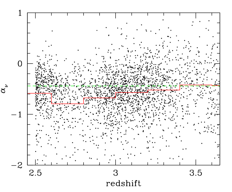
Figure 4: The distribution of continuum indices as a function of redshift for quasars with $z~{}\hbox to0.0pt{$<$\hss}{\lower 4.30554pt\hbox{$\sim$}}3.6$. The histogram indicates the mean in bins of $\Delta z=0.2$. The averaged continuum index is $-0.59\pm 0.35$. The horizontal dashed line is $\alpha_{\nu}=-0.44$, the mean slope reported by Vanden Berk et al. (2001) and B03.

Following P93 and B03, we assume that the shape of the quasar continuum is the superposition of a single power law and emission lines. Our approach, however, differs from theirs in that we include variation in continuum indices. To proceed, we select wavelength windows free of emission lines and fit a power law continuum on a spectrum-by-spectrum basis. Although there are essentially no emission-line free regions (Vanden Berk et al. 2001), we use the rest wavelength intervals 1450-1470Å and 1975-2000Å (e.g. Telfer et al. 2002). A visual inspection of the fitted continuum has convinced us that this prescription provides a reasonable description of the individual continua. Note, however, that low redshift SDSS composites indicate that the window 1975-2000Å may be contaminated by FeII emission (see Fig.6 of Vanden Berk et al. 2001). This would cause us to infer continua softer than the actual ones (Telfer et al. 2002). The distribution of continuum indices is plotted in Fig. 4 for quasars with $z~{}\hbox to0.0pt{$<$\hss}{\lower 4.30554pt\hbox{$\sim$}}3.6$. It is not possible to perform a similar measurement of the continuum at higher redshift because of the spectroscopic red limit of 9200Å . The histogram indicates the mean value of $\alpha_{\nu}$ in bins of $\Delta z=0.2$. The average power law slope of the subsample is -0.59 (median -0.53) with a 1$\sigma$ dispersion of 0.36. This is in good agreement with the mean slope reported by Vanden Berk et al. (2001) and B03, $\alpha_{\nu}=-0.44$, and with values found in optically selected samples (e.g. Francis et al. 1991; Natali et al. 1998). At $z~{}\hbox to0.0pt{$>$\hss}{\lower 4.30554pt\hbox{$\sim$}}3.6$, fitting a continuum proves difficult due to the relatively low signal-to-noise, and the short continuum baseline available redward of the op emission line. Using the rest wavelength range redward of the CIV emission line, $\sim$1600-1700Å  then plays a significant role in determining the slope (Schneider et al. 2001). We have tried to fit the regions near 1260Å and 1650Å  as done in Schneider et al. (2001). As a consistency check, we have remeasured the continuum indices of quasars with $z~{}\hbox to0.0pt{$<$\hss}{\lower 4.30554pt\hbox{$\sim$}}3.6$ using that rest frame region. We have found that this method gives steeper indices than those inferred from the rest wavelength region 1460-2000Å, in agreement with Vanden Berk et al. 2001. We have tried several other alternatives but none of them gave satisfactory results. We have therefore opted for a constant slope $\alpha_{\nu}=-0.44$ when the quasar redshift is $z~{}\hbox to0.0pt{$>$\hss}{\lower 4.30554pt\hbox{$\sim$}}3.6$, implicitly assuming that the mean continuum index does not change much with redshift. Note that this will affect solely our measurement of the Ly$\alpha$ flux PDF at $z=3.9$.

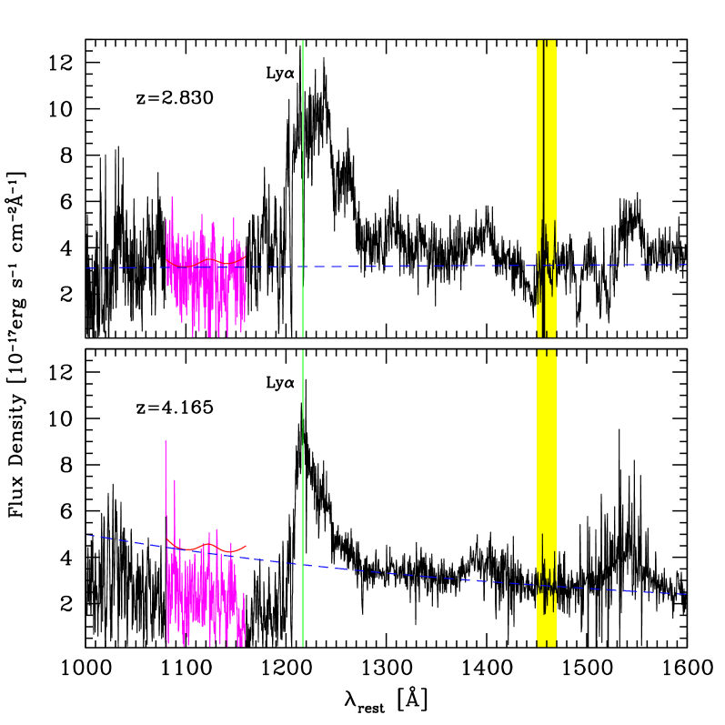
Figure 5: Two quasar spectra of the DR3 sample plotted as a function of wavelength in the rest frame. The dashed line shows the power law fit. The continuum index is $\alpha_{\lambda}=0.10$ and -1.56 for the low and high redshift spectrum, respectively. The shaded area indicates the wavelength range 1450-1470Å used to normalise the continuum. The solid curve shows the continuum in the Ly$\alpha$ forest, including the emission lines. We analyse the Ly$\alpha$ forest in the wavelength region 1080-1160Å.

We follow P93, Zheng et al. (1997) and normalise the QSO continuum in the rest-wavelength range $1450-1470\AA$ to have the same flux as the observed spectra. To account for the emission lines blueward of 1216Å, we adopt the parametrisation of B03,

$${\cal C} = c_{0}\left(\frac{\lambda_{\rm rest}}{\lambda_{0}}\right)^{\alpha_{\lambda}}+c_{2}\exp\left[-\frac{\left(\lambda_{\rm rest}-c_{3}\right)^{2}}{2c_{4}^{2}}\right]$$ (8)

$$+c_{5}\exp\left[-\frac{\left(\lambda_{\rm rest}-c_{6}\right)^{2}}{2c_{7}^{2}}\right]$$

$$+c_{8}\exp\left[-\frac{\left(\lambda_{\rm rest}-c_{9}\right)^{2}}{2c_{10}^{2}}\right]\;,$$

where ${\cal C}$ is the continuum as a function of the rest wavelength $\lambda_{\rm rest}$. The continuum slope $\alpha_{\lambda}=-\left(2+\alpha_{\nu}\right)$ is estimated spectrum-by-spectrum as explained above. The position of the peak of the Ly$\alpha$ emission line ($c_{9}$=1215.67Å), and the other two emission lines seen in the composite spectrum ($c_{3}$=1073Å and $c_{6}$=1123Å) are fixed to reduce the number of free parameter. The remaining six parameters can be obtained, e.g., from a $\chi^{2}$ minimisation of the difference between the simulated and observed composite spectra (B03). Here, we have simply adopted the best fit values of B03 that were obtained for a constant power law slope $\alpha_{\lambda}=-1.56$. Two examples of spectra and continuum are shown in Fig. 5. The solid curve indicates our fit (8) to the continuum in the Ly$\alpha$ forest region. Note that the continuum index of the low redshift spectrum, $\alpha_{\lambda}=0.10$, differs noticeably from the average slope of -1.56.

4.3 The probability distribution of the transmitted flux

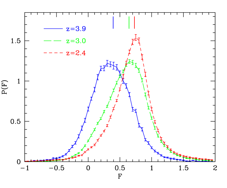
Figure 6: The probability distribution of the transmitted flux $F$ is computed from the DR3 sample and plotted in differential form. Results are presented for three different redshift intervals of length $\Delta z=0.2$ centered at $z=3.9$, 3.0 and 2.4. Vertical bars indicate the mean transmitted flux $\bar{F}$ in each redshift interval. The error bars are computed from a jackknife estimate

Once we have taken out the contribution of the continua from our quasar spectra (on a spectrum-by-spectrum basis), we compute $P(F)$, the probability distribution of the transmitted flux $F$. Since a substantial fraction of the pixels has a transmitted flux which lies outside the interval $0\leq F\leq 1$, we use 60 bins of width $\Delta F=0.05$ with the first centered on $F=-1$ and the last on $F=2$. The first and last bins include the few additional points with $F<-1$ and $F>2$, respectively. Results are shown in the top panel of Fig. 6 for three different redshift intervals as defined in Table 2. These redshift intervals are centered on $z=3.9$, 3.0 and 2.4, allowing a direct comparison with the high resolution measurements of McDonald et al. (2000). It is important to note that each redshift interval covers a narrow redshift range of $\Delta z=0.2$. This is in order to reduce the impact of evolution with redshift in each interval. The vertical bars mark the mean transmitted flux $\bar{F}$ in each redshift interval, obtained by averaging the individual flux pixels (without weighing them according to their noise). We have $\bar{F}\simeq 0.39$, 0.64 and 0.73 respectively. These values are significantly lower than those inferred from the high resolution sample, $\bar{F}\simeq 0.45$, 0.69 and 0.82 (M00). The high noise level smoothes severely the PDF relative to that of high-resolution observations (compare with the right panels of Fig. 2), and is responsible for the existence of pixels with $F>1$ and $F<0$. The effect is strongest at $z=3.9$, where the average signal-to-noise in the Ly$\alpha$ forest is lowest (see Figure 3).

The errors bars attached on the measured PDF shown in Fig. 6 are obtained from a jackknife estimate of the covariance matrix $C_{ij}$, which includes Ly$\alpha$ forest fluctuations and measurement noise. These diagonal elements are plotted as dashed curves in Fig. 7. Note that the curves at redshift $z=2.4$ and 3 have been shifted vertically by 0.04 and 0.02 respectively for clarity. As it is difficult to estimate cleanly off-diagonal terms or diagonal elements lying in the tails of the PDF with such an estimator, we have also computed the errors from the dispersion across many realisations of mock spectra with properties similar to that of the observed sample (cf. Section §2). In particular, the mock samples have exactly the same total wavelength coverage (number of pixels) as the actual sample. The parameters assume the best fit values inferred in  §3, with a mean flux $\langle F\rangle=0.5$, 0.7 and 0.8. Our estimates of $\sqrt{C_{ii}}$ are shown in Fig. 7 as dashed and solid curves, respectively. They are consistent with each other at redshift $z~{}\hbox to0.0pt{$>$\hss}{\lower 4.30554pt\hbox{$\sim$}}3$. However, at lower redshift, the errors inferred from the observed sample are significantly larger than those obtained from the mocks. We have found that the jackknife estimator, when applied to a single mock SDSS sample, predicts errors similar to those inferred from a large number of mock realisations. Therefore, this discrepancy probably reflects errors in the measurement of the flux PDF, errors in the modelling of low resolution SDSS spectra, or/and the failure of the lognormal model to adequately describe the low redshift Ly$\alpha$ forest (e.g. Nusser & Haehnelt 1999). Note that the off-diagonal terms of the covariance matrix are negligible presumably because the large noise washes out correlations among the data points. The correlation coefficient $r_{ij}=C_{ij}/\sqrt{C_{ii}C_{jj}}$ is no larger than $|r_{ij}|~{}\hbox to0.0pt{$<$\hss}{\lower 4.30554pt\hbox{$\sim$}}0.01$ for $i\neq j$. This is in contrast with high signal-to-noise measurements of the PDF (see e.g. M00; Lidz et al. 2005) where off-diagonal terms in the covariance matrix are significant due to the strong correlation among data points.

Table 2: The redshift intervals considered in this paper. The last two columns show the number of spectra and pixels included in each interval.

$\langle z\rangle$	$z_{\rm min}$	$z_{\rm max}$	$N$ of spectra	$N$ of pixels
2.4	2.3	2.5	942	127212
3.0	2.9	3.1	1082	133371
3.9	3.8	4.0	281	29003

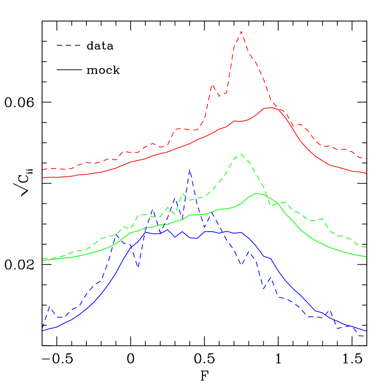
Figure 7: A comparison between the diagonal terms $\sqrt{C_{ii}}$ of the covariance matrix computed from the data with a jackknife estimate (dashed curve), and the $\sqrt{C_{ii}}$ obtained from a large number of mock catalogues (solid curves). Results are shown at $z=2.4$, 3 and 3.9 (from bottom to top). The curves at $z=2.4$ and 3 have been shifted vertically for clarity.

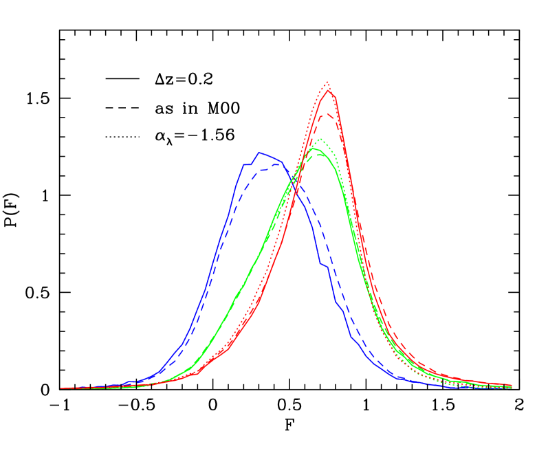
Figure 8: The probability distribution of the transmitted flux for the redshift intervals adopted in M00 (dashed curves), for the redshift intervals considered in this work (solid curves), and for a fixed continuum index $\alpha_{\lambda}=-1.56$ (dotted curves). The redshift intervals are centered at $z=2.4$, 3 and 3.9.

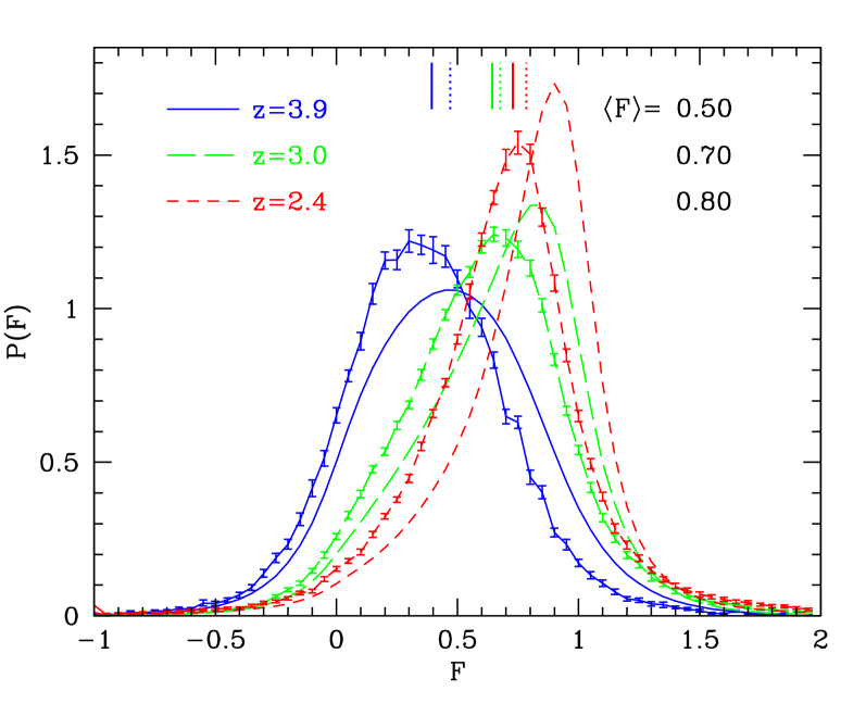
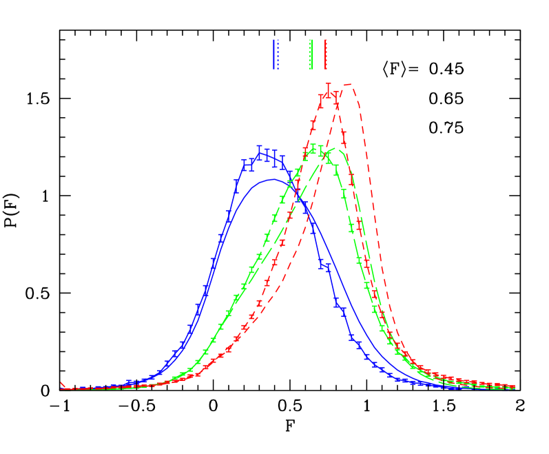
Figure 9: A comparison between the observed and mock Ly$\alpha$ flux PDFs of low-resolution QSOs at redshift $z=3.9$, 3 and 2.4. The error bars are attached to the observed PDF only. The solid and dotted vertical bars indicate the observed and predicted mean flux $\bar{F}$. In the left panel, the models have $\langle F\rangle=0.50$, 0.70 and 0.80. In the right panel, the mean flux parameter is $\langle F\rangle=0.45$, 0.65 and 0.75, respectively.

In Section §3, we have constrained the model parameters from measurements of the flux PS and PDF which are fairly representative of the true statistics at redshift $z=2.4$, 3 and 3.9. However, these measurements are averaged in relatively large redshift bins, over which the evolution of the Ly$\alpha$ forest is significant. It is, therefore, prudent to examine the extent to which our measurements of the PDF at redshift $z=2.4$, 3 and 3.9 are sensitive to the adopted redshift intervals. We have thus computed the PDF of the transmitted flux for the redshift intervals adopted in M00 ($2.09\leq z\leq 2.67$, $2.67\leq z\leq 3.39$ and $3.39\leq z\leq 4.43$). The results are shown as dashed curves in Fig. 8. They are compared to our fiducial measurement of the probability distribution function obtained with a redshift interval $\Delta z=0.2$ (solid curves). The difference is largest at $z=3.9$, where the sharp decrease in the number of pixels at $z~{}\hbox to0.0pt{$>$\hss}{\lower 4.30554pt\hbox{$\sim$}}4$ (Fig. 3) and the strong increase in the flux over the range $3.5<z<4.5$ conspire to raise the average mean flux by 10 per cent. At $z=2.4$, the height of the peak is decreased by about 10 per cent. Obviously, the strength of the effect depends on the exact shape of the selection function (see Fig. 3). This result suggests that the PDF measured by M00 from a sample of Keck quasars is also likely to be biased with respect to that measured in intervals of size $\Delta z=0.2$. We will discuss this point later in Section §6. In Fig. 8, the dotted curves show the PDF at $z=3$ and 2.4 for a fixed value of the continuum index, $\alpha_{\lambda}=-1.56$. Interestingly, accounting for variation in the continuum slope has a noticeable impact on the PDF, especially on the average mean flux. For a fixed index $\alpha_{\lambda}=-1.56$, the mean flux at $z=3$ and 2.4 is $\bar{F}=0.626$ and 0.675, respectively $\sim$3 and $\sim$7 per cent lower than the values of 0.643 and 0.728 obtained with a spectrum-by-spectrum fitting. We have also changed the interval defining the Ly$\alpha$ forest, and found that the measured PDF is robust to the wavelength range as long as intrinsic features to the quasar are excluded.

5 comparison between observed and mock spectra

In this Section, we compare the flux probability distribution of low resolution mock spectra with that inferred from the DR3 sample.

5.1 The PDF of the transmitted flux

We generate mock catalogues of low resolution spectra for the best-fitting values of the parameters obtained in Section §3. We adopt a grid similar to that used in §3. The comoving length of a single mock spectrum is typically $~{}\hbox to0.0pt{$>$\hss}{\lower 4.30554pt\hbox{$\sim$}}1000\ {\rm{\it h}^{-1}Mpc}$. We account for instrumental resolution, noise and the presence of strong absorption systems according to the procedure outlined in §2.3.

The observed and mock PDFs are compared in the left panel of Fig. 9. Error bars are attached to the observed PDF only. The mock spectra have a mean flux parameter $\langle F\rangle=0.50$, 0.70 and 0.80 at $z=3.9$, 3 and 2.4. This corresponds to an ’effective’ (i.e. including strong absorption systems) mean flux $\bar{F}\approx$ 0.47, 0.67 and 0.78 respectively. The solid and dotted vertical bars indicate $\bar{F}$ for the observed and simulated samples, respectively. $\bar{F}$ is on average larger by $~{}\hbox to0.0pt{$>$\hss}{\lower 4.30554pt\hbox{$\sim$}}10$ per cent in the mock samples. The mock PDF correctly accounts for the shape and redshift evolution measured in the data. However, the agreement is poor given the small error bars. At $z~{}\hbox to0.0pt{$<$\hss}{\lower 4.30554pt\hbox{$\sim$}}3$ in particular, the peak in the flux probability distribution is significantly more pronounced in the mock PDF than in the observation.

5.2 Sensitivity to the mean flux, noise level, and the presence of strong absorption systems

Since the synthetic spectra have been constrained to reproduce the observed PDF and PS measured in high resolution data, the shortcomings of the lognormal model are unlikely responsible for the difference between the observed and mock PDFs. The disagreement must originate either in the transformation of the idealised mocks into realistic looking SDSS spectra, or in the measurement of the Ly$\alpha$ flux probability distribution of the SDSS sample. We now discuss a number of systematics that may cause the difference between data and simulation.

5.2.1 Mean flux

Fig. 9 examines the sensitivity of the SDSS PDF to the mean flux level. The right panel shows the mock PDF of the best-fitting models listed in Table 1, with $\langle F\rangle=0.45$, 0.65 and 0.75 at $z=3.9$, 3 and 2.4, respectively (This corresponds to $\bar{F}=$0.42, 0.63 and 0.74). These values are marginally consistent with those inferred from high resolution measurements of the Ly$\alpha$ forest. Note, however, that the $z~{}\hbox to0.0pt{$<$\hss}{\lower 4.30554pt\hbox{$\sim$}}3$ models poorly account for the observed Ly$\alpha$ flux PDF and PS. Changing $\langle F\rangle$ affects both the shape and the peak position $F_{\rm peak}$ of the PDF. The right panel of Fig. 9 demonstrates that a $\sim$10 per cent decrease in $\langle F\rangle$ improves the agreement with the observed PDF, especially with the observed mean flux $\bar{F}$. Notwithstanding this, at $z~{}\hbox to0.0pt{$<$\hss}{\lower 4.30554pt\hbox{$\sim$}}3$, the mock PDF still peaks at a higher value of the transmitted flux $F$ than the observed PDF. The effect is strongest at $z~{}\hbox to0.0pt{$<$\hss}{\lower 4.30554pt\hbox{$\sim$}}3$. Consequently, lowering the mean flux level $\langle F\rangle$ in the mock spectra can at best partly alleviate the tension between the mock and observed PDFs. It should also be noted that, in the mock PDF, the mean flux value $\bar{F}$ is significantly lower than $F_{\rm peak}$ at $z~{}\hbox to0.0pt{$<$\hss}{\lower 4.30554pt\hbox{$\sim$}}3$. This follows from the fact that the PDF is asymmetric around $F_{\rm peak}$, decreasing sharply for $F~{}\hbox to0.0pt{$>$\hss}{\lower 4.30554pt\hbox{$\sim$}}F_{\rm peak}$.

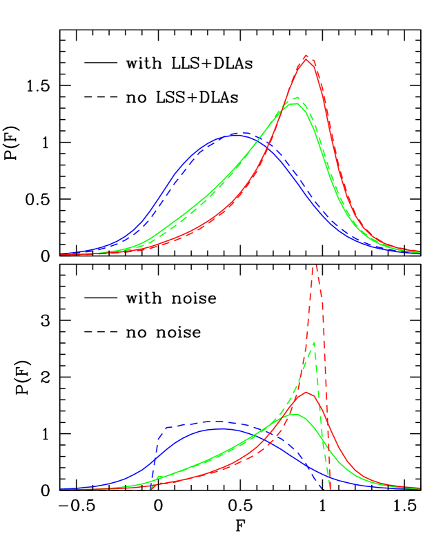
Figure 10: Top panel : Impact of strong absorption systems on the flux PDF. The solid and dashed curves show the PDF with and without strong absorption systems. Bottom panel : Sensitivity of the PDF to the noise level. The dashed curves show the PDF when the noise is set to zero. The mock PDF have $\langle F\rangle=0.5$, 0.7 and 0.8 for $z=3.9$, 3 and 2.4, respectively.

5.2.2 Metal lines and strong absorption systems

The probability distribution of the flux may be affected by the presence of metal lines and strong absorption systems (e.g. Schaye et al. 2003; Viel et al. 2004b). The top panel of Fig. 10 investigates the sensitivity of the PDF to the presence of strong absorption systems. The inclusion of strong absorption systems (cf. Section §2.3) decreases the mean transmitted flux $\bar{F}$ of the low resolution mock spectra by $\sim 3-6$ per cent in the redshift range $2.5~{}\hbox to0.0pt{$<$\hss}{\lower 4.30554pt\hbox{$\sim$}}z~{}\hbox to0.0pt{$<$\hss}{\lower 4.30554pt\hbox{$\sim$}}4$. We confirm the results of McDonald et al. (2005b) who find that the Ly$\alpha$ forest is not very sensitive to the details of the strong absorption lines, except when the damping wings become important. Regarding the presence of metal lines, the typical metallicity of the low-density IGM remains largely unknown, although early statistical analysis based on pixel optical depth methods seemed to indicate that there is CIV and OVI associated with the low-column density Ly$\alpha$ forest (Cowie & Songaila 1998; Ellison et al. 2000; Schaye et al. 2000a). More recent studies appear to refute these claims, and suggest that the volume filling fraction of metals is small, $\sim 5$ per cent, in the redshift range $2<z<4$ (Pieri & Haehnelt 2003; Aracil et al. 2004). Clearly, at redshift $z~{}\hbox to0.0pt{$>$\hss}{\lower 4.30554pt\hbox{$\sim$}}3$, absorption in the Ly$\alpha$ forest region is strongly dominated by the Ly$\alpha$ resonant transition, and the impact of metals on the flux PDF is likely to be negligible. At lower redshift however, metals contribute more significantly to the absorption. From a sample of quasars at mean redshift $z=1.9$, Tytler et al. (2004) have estimated that metal lines absorb $\sim$2.5 per cent of the flux in the Ly$\alpha$ forest. However, this falls short of explaining the $~{}\hbox to0.0pt{$>$\hss}{\lower 4.30554pt\hbox{$\sim$}}10$ per cent different found between the simulated and predicted PDFs.

5.2.3 Noise level

The bottom panel of Fig. 10 illustrates the sensitivity of the flux probability distribution to the amount of noise. The solid curve shows the mock PDF obtained with our default noise level $\sigma_{p}$ given by the SDSS reduction pipeline (cf. §2.3). The dashed curve shows the PDF when the noise is set to zero. The large pipeline noise smoothes the idealized, noise-free PDF significantly. A few per cent change in $\sigma_{p}$ noticeably affects the shape of the PDF. In this respect, at $z~{}\hbox to0.0pt{$<$\hss}{\lower 4.30554pt\hbox{$\sim$}}3$, increasing $\sigma_{p}$ would lower the peak, and bring the PDF in better agreement with the observations. Note, however, that changing the noise level leaves the mean flux $\langle F\rangle$ unchanged.

Fig. 3 shows that the distribution of signal-to-noise in our sample is broad. To assess the extent to which the shape of the measured PDF is affected by the noise level, we split the sample based on the mean signal-to-noise in the Ly$\alpha$ forest. The upper panels of Fig. 11 show the probability distribution of the Ly$\alpha$ flux for spectra with $S/N>4$ (left panels) and $S/N<4$ (right panels) for our fiducial continuum and noise level. Results are shown solely for $z=3$ and 2.4, as higher redshift spectra tend to have low $S/N$ ratios (see Figure 3). The observed PDF is plotted with errorbars. Cosmic variance errors have been computed separately for both subsamples, which include approximately the same number of data points ($\sim 6\times 10^{4}$ pixels). The upper right panels show that the peak height of the observed flux probability distribution of low $S/N$ spectra is larger at $z=3$ than at $z=2.4$, while high $S/N$ spectra show the opposite trend. This is presumably due to the large noise which dominates the signal, and gives the PDF a nearly Gaussian shape.

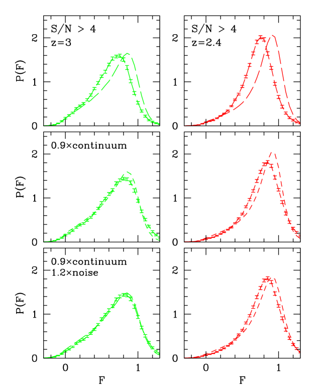
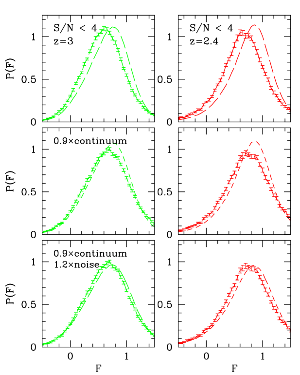
Figure 11: A comparison between the measured (curves with errorbars) and mock probability distributions of the Ly$\alpha$ flux at $z=3$ and 2.4. The left and right panels are for spectra with $S/N$ ratios greater than and less than 4, respectively. The upper panels show results for our default noise and continuum. In the middle panels, the fiducial continuum has been decreased by 10 per cent. In the bottom panels, both the continuum and the noise have been rescaled by a factor 0.9 and 1.2, respectively.

Since the SDSS spectral resolution varies in the range $R\sim 1800-2100$, we have also computed the PDF with an lower instrumental resolution of 150$\ {\rm km\,s^{-1}}$ (FWHM). At $z~{}\hbox to0.0pt{$<$\hss}{\lower 4.30554pt\hbox{$\sim$}}3$, a decrease of  $<$$\sim$ 10 per cent in the instrumental resolution has a relatively small impact on the flux probability distribution.

5.3 Changing the continuum and noise levels

Decreasing the mean flux, accounting for metal lines or increasing the noise level in the mock spectra can only partly account for the difference between the observed and simulated PDF.

In the data, the main sources of systematic errors are inaccuracies in the continuum fitting of the spectra. Given the large degeneracy between the amount of absorption and the continuum level in the Ly$\alpha$ region, it is unclear whether the single power law approximation can be extended shortward of the Ly$\alpha$ emission line. Low redshift spectroscopic measurements show indeed that there is a break around $1000-1300\AA$ in the slope of the mean quasar continuum. They indicate that the continuum turns over in that rest frame region, from $\alpha_{\nu}>-1$ longward of the break to $\alpha_{\nu}<-1$ shortward (e.g. Zheng et al. 1997; Telfer et al. 2002). The exact location of the break is, however, difficult to determine due to the presence of emission lines. This turnover is neither accounted for in the continuum extrapolation method of P93 and B03, nor in our procedure. As noticed by by Kim et al. (2001) and Meiksin, Bryan & Machacek (2001), this may lead to an underestimation of $\langle F\rangle$ that could be as large as $~{}\hbox to0.0pt{$<$\hss}{\lower 4.30554pt\hbox{$\sim$}}7$ per cent (Seljak, McDonald & Makarov 2003). Consequently, we will now relax the assumption of a single power law. Since there are large uncertainties in the behaviour of the continuum blueward of 1216Å, we have not looked for a parametric form of the turnover. Instead, we have simply assumed that the true continuum is a rescaled version of our fiducial continuum ${\cal C}$, ${\cal C}_{\rm true}=\beta_{c}\,{\cal C}$, where $\beta_{c}$ is a mean correction factor which we will attempt to constrain. We ignore any possible dependence on redshift and quasar luminosity.

The middle panels of Fig. 11 show the observed probability distribution when the continuum in the Ly$\alpha$ region is rescaled by 90 per cent ($\beta_{c}=0.9$). It is compared to the mock PDF obtained with the fiducial noise level. Note that the errors in the observed transmitted flux depend on the continuum level, as $F=I_{\rm obs}/I_{\rm cont}$. The 10 per cent decrease in the continuum translates into a comparable increase in the observed mean flux, which is now $\bar{F}=0.69$ and 0.80 at $z=3$ and 2.4, respectively. Notwithstanding this, the peak in the simulated PDF is still more pronounced than in the observed PDF. A further decrease of the continuum does not improve the agreement. In fact, unless the actual mean flux is significantly lower than that inferred from high resolution data, a substantial increase in the noise level is needed to reproduce the smooth shape of the observed PDF.

The bottom panel of Fig. 11 demonstrates that the agreement with the data is substantially improved if the pipeline noise is increased by $\sim$20 per cent. The agreement is however better at $z=3$ than at $z=2.4$, where the mock PDF still appears to be shifted to larger values of $F$ when compared to the observed PDF. This may be due to too large a mean flux level $\langle F\rangle$. It may also reflect the poor performance of the lognormal model at redshift $z<3$ (cf. Table 1).

The correction factor $\beta_{c}$ that quantifies the deviation from a power law is expected to vary from spectrum to spectrum. It also probably depends on the rest frame wavelength $\lambda_{\rm rest}$. Using a constant value of $\beta_{c}$ smoothes the flux probability distribution as compared to the “true” PDF, thereby mimicking the effect of a larger noise. We have found that the introduction of a 10 per cent scatter (Gaussian deviate) in the continuum level of $z=3$ mock spectra smoothes the flux PDF on a level comparable to a 20 per cent increase in the noise. At $z=2.4$, this corresponds to an even larger increase in the noise, presumably because the average signal-to-noise is lower. Therefore, an increase in the mean noise level can account for both a larger noise per pixel and variations in the continuum. We will come back to this point in §6.

5.4 The best-fitting models

The agreement between the mock and observed PDFs of low resolution spectra can be substantially improved with a simultaneous decrease in the continuum level, and an increase in the noise per pixel. We will now attempt to quantify the correction needed in the continuum level and noise estimate. In spite of the large uncertainties in the actual noise level, we assume that the true noise $\sigma_{\rm true}$ differs from the pipeline noise by a constant factor, $\sigma_{\rm true}=\beta_{n}\,\sigma_{p}$. Similarly, we take the true continuum in the Ly$\alpha$ region to be a scaled version of the fiducial continuum, ${\cal C}_{\rm true}=\beta_{c}\,{\cal C}$. We let $\beta_{n}$ and $\beta_{c}$ vary in the range $1\leq\beta_{n}\leq 1.8$ and $0.8\leq\beta_{c}\leq 1$. We take $0.65\leq\langle F\rangle\leq 0.75$ and $0.75\leq\langle F\rangle\leq 0.85$ at $z=3$ and 2.4, respectively. For each value of $\beta_{c}$, we compute the PDF of the Ly$\alpha$ transmitted flux from the SDSS quasars with $S/N>4$. We store the distribution of noise per pixel values, $\delta F$, as a function of $\beta_{c}$ since the average $\delta F$ increases with decreasing value of $\beta_{c}$. To compute the mock PDF, we let the filtering wavenumber $k_{\rm F}$ and the adiabatic index $\gamma$ assume the best-fitting values obtained in  §3 as a function of $\langle F\rangle$, but for a fixed value of the temperature, $\hat{T}_{4}=1.5$. We compute the flux probability distribution for each choice of $(\beta_{c},\beta_{n},\langle F\rangle)$. The goodness of fit of the models is obtained by minimizing a $\chi^{2}$ statistic as in §3. The shaded region in Fig. 12 indicates the SDSS data points we use in the calculation of $\chi^{2}$. We discard the data points falling in the  $<$$\sim$10 per cent lower and $~{}\hbox to0.0pt{$<$\hss}{\lower 4.30554pt\hbox{$\sim$}}10$ per cent upper tails of the flux distribution. We also include in the $\chi^{2}$ minimisation the best-fitting values of $\chi^{2}$ as a function of $\langle F\rangle$ obtained from the measurements of M00 (cf. §3). The best-fitting values of the parameters are $(\beta_{c},\beta_{n},\langle F\rangle)$=(0.87,1.51,0.72) and (0.84,1.55,0.84), and correspond to a reduced chi-squared $\chi^{2}/\nu=1.03$ and 1.54 at $z=3$ and 2.4 respectively. The best-fitting models are plotted in Fig. 12 as short and long dashed curves. Restricting the $\chi^{2}$ minimisation to the SDSS data set solely does not affect noticeably the central values of $\beta_{c}$, $\beta_{n}$ and $\langle F\rangle$.

6 Discussion

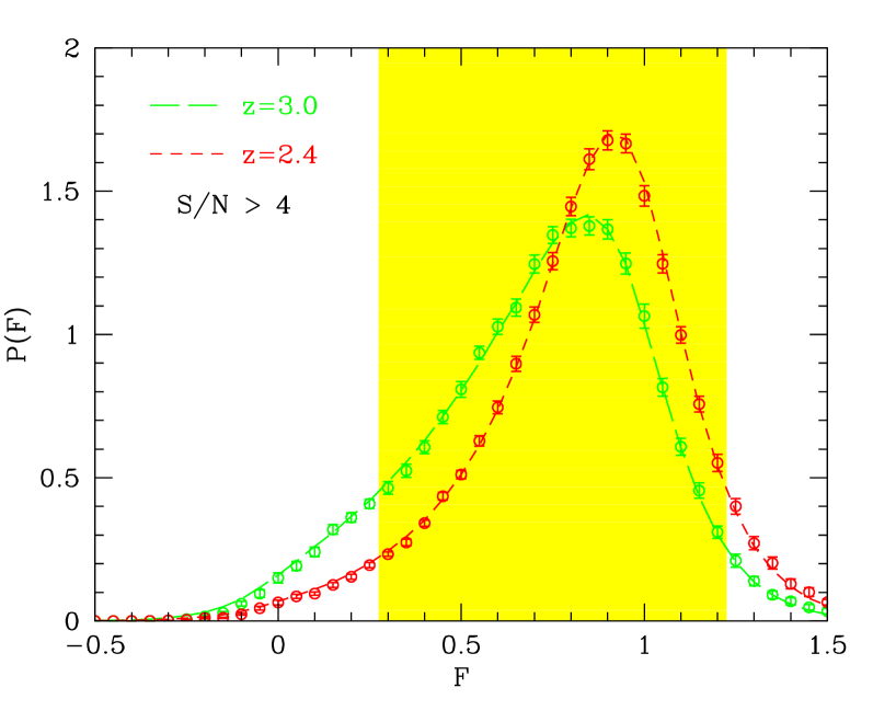
Figure 12: The best-fitting Ly$\alpha$ flux PDF at redshift $z=3$ and 2.4. The short and long dashed curves show the best-fitting mock PDF at $z=3$ and 2.4 respectively. The continuum level, noise estimate and mean flux parameter $\langle F\rangle$ have been varied to obtain the best-fitting models. The symbols with errorbars show the observed flux PDF of spectra with a signal-to-noise ratio greater than 4. The shaded region indicates the SDSS data points used to compute the value of $\chi^{2}$. We also include in the chi-squared the measurements of M00 as described in §3.

6.1 Systematics in the measurements

Section §5.4 argues that the continuum level needs to be lowered by 10-15 per cent, and the pipeline noise increased by $\sim$ 50 per cent so that the mock PDF matches the data. The noise correction is significantly larger than that inferred by McDonald et al. (2006) and Burgess (2004) by differencing multiple exposures of the same quasar. They have found that the SDSS pipeline underestimates the true errors by 5-10 per cent on average. Although we do not have access to additional exposures, we can take advantage of the relative smoothness of the spectra redward of the Ly$\alpha$ emission line, and estimate the noise in, e.g., the rest-frame wavelength interval 1450-1470Å as the rms variance $\sigma_{f}$ of the flux around the continuum. Then, $\sigma_{f}$ can be compared to the average pipeline noise variance, $\bar{\sigma}_{p}$, in the same region. The value of $\bar{\sigma}_{p}$ is obtained by squaring the individual pixel noise estimates, computing the average of these squared values, and taking the square root. The distribution of ratios $\sigma_{f}/\bar{\sigma}_{p}$ is shown in Fig. 13 for the individual spectra. The solid histogram indicates the mean in bins of $\Delta z=0.2$. The median, which is less sensitive to outliers, is also shown as the dashed histogram. The mean ratio does not evolve significantly with redshift, although Fig. 13 suggests that it might be bigger at higher redshift. In the range $z\sim 2.5-4$, $\sigma_{f}$ is on average 10-15 per cent larger than $\bar{\sigma}_{p}$. This is comparable to the excess noise contribution inferred by McDonald et al. (2006) and Burgess (2004). It is unclear to which extent $\sigma_{f}/\bar{\sigma}_{p}$ reflects the excess noise contribution in the Ly$\alpha$ forest. However, the fact that McDonald et al. (2006) find the same excess noise power in the region 1268-1380Å as they do in the Ly$\alpha$ forest suggests that the fraction of extra noise does not depend strongly on $\lambda_{\rm rest}$. Consequently, the 50 per cent increase in the noise level most probably arises from residual variations in the continua of quasars that are not accounted for by our spectrum-to-spectrum continuum fitting. In §5.3, we have found that the introduction of a 10 per cent scatter in the continuum level of $z~{}\hbox to0.0pt{$<$\hss}{\lower 4.30554pt\hbox{$\sim$}}3$ mock spectra smoothes the flux PDF on a level comparable to a 20-30 per cent increase in the noise. Hence, we believe that a reasonable $\sim$20 per cent scatter in the continuum level can account for the smooth shape of the SDSS PDF if the noise excess correction is no larger than  $<$$\sim$10 per cent. To proceed further, one could add another free parameter describing the residual scatter in the continuum and perform again the $\chi^{2}$ minimisation of §5.4. However, given our approximate characterisation of the continuum and noise level, we have not examined this issue here.

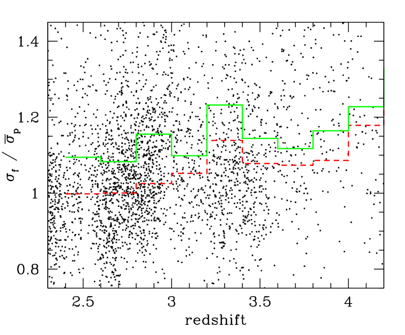
Figure 13: The distribution of ratios $\sigma_{f}/\bar{\sigma}_{p}$ in the rest-frame wavelength interval $1450-1470\AA$, where $\sigma_{f}$ is the rms flux variance, and $\bar{\sigma}_{p}$ is the mean SDSS pipeline noise estimate (see text). The solid and dashed histograms indicate the mean and median in bins of $\Delta z=0.2$.

Systematics errors arising from continuum fitting in the measurements of M00 may bias our best-fitting values of the parameters, and thereby affect the PDF of mock SDSS spectra. However, a comparison with hydrodynamical simulations of the Ly$\alpha$ forest indicates that the M00 measurements are robust to continuum errors for transmitted flux values $F~{}\hbox to0.0pt{$<$\hss}{\lower 4.30554pt\hbox{$\sim$}}0.8$. The large redshift range covered by the M00 bins may also affect our results. The latter have been obtained using small redshift intervals, $\Delta z=0.2$, to avoid dealing with the (poorly constrained) redshift dependence of the model parameters. Fig. 8 shows that our measurement of the PDF of SDSS quasars is sensitive to the redshift extent of the bins. The significance of this effect in measurements of the PDF from high-resolution quasars is unknown, though it could be easily estimated from the few tens of spectra available so far.

6.2 Systematics in the model

The lognormal model of the IGM allows us to create very long, realistic mock spectra of the Ly$\alpha$ forest. However, the model has several shortcomings. It neglects any possible scatter in the temperature-density relation of the low density IGM as a results of shocks and inhomogeneous helium reionization. It also assumes an uniform ultraviolet (UV) background, and a filtering length that is independent of the local gas density and temperature. Furthermore, it ignores any galactic feedback.

Hydrodynamical simulations predict that shock heating should drive a significant fraction of the baryons into the warm-hot phase of the intergalactic medium (WHIM) at low redshift. At the present epoch, this fraction might be as large as 40 per cent (e.g. Cen & Ostriker 1999; Davé et al. 2001; see also Nath & Silk 2001). At redshift $z\sim 3$ however, these simulations indicate that this fraction falls below 10 per cent, and that most of the WHIM baryons resides in overdensities $\delta_{\rm b}~{}\hbox to0.0pt{$>$\hss}{\lower 4.30554pt\hbox{$\sim$}}10$ (Davé et al. 2001). Hence, shock heating should have a rather weak impact on the low density IGM at $z\approx 3$.

Inhomogeneities in the UV background may also affect the power spectrum and the PDF of the Ly$\alpha$ flux (Zuo 1992; Fardal & Shull 1993; Croft et al. 2002a). At $z<4$ however, fluctuations due to the finite number of sources are only at the few percent level because of the small attenuation length (Croft 2004; Meiksin & White 2004; McDonald et al. 2005b). Recent measurements of the Ly$\alpha$ absorption near Lyman-break galaxies (Adelberger et al. 2003) are taken as evidence for the existence of dilute and highly ionised gas bubbles caused by supernovae-driven winds. Notwithstanding this, simulations indicate that their small filling factor results in a moderate impact on statistics of the Ly$\alpha$ forest such as the power spectrum or the PDF of the transmitted flux (e.g. Croft et al. 2002a; Weinberg et al. 2003; Desjacques et al. 2004; McDonald et al. 2005b; Desjacques, Haehnelt & Nusser 2006). They may, however, have a large impact on the number and properties of absorption lines with $N_{{}_{\rm HI}}~{}\hbox to0.0pt{$>$\hss}{\lower 4.30554pt\hbox{$\sim$}}10^{16}\ {\rm cm^{-2}}$ (Theuns, Mo & Schaye 2000; Theuns et al. 2002a).

The use of a polytropic equation of state and a constant filtering length to mimic the temperature and pressure of the gas has been shown to produce results comparable to detailed hydrodynamical simulations (Petitjean et al. 1995; Croft et al. 1998; Gnedin & Hui 1998; Meiksin & White 2001). Yet, patchy helium reionization can cause significant scatter in the temperature-density relation (e.g. Gleser et al. 2005). Furthermore, in light of the results of Viel, Haehnelt & Springel (2006), we expect significant differences between the Ly$\alpha$ statistics predicted by full hydrodynamical simulations and from the lognormal model. Consequently, the constraints on, e.g., the temperature and adiabatic index which can be inferred from the high resolution data should be taken with caution. In particular, the linear amplitude $\sigma_{\rm L}$ is an effective normalisation which cannot be directly related to the actual rms variance of the gas distribution. However, once the parameters of the lognormal model are constrained so as to reproduce the observed Ly$\alpha$ flux power spectrum and probability distribution measured in M00, the disagreement seen in Fig. 9 must arise either from systematics errors in the measurement of the PDF or in the conversion of the idealised mocks into realistic looking SDSS spectra.

7 Conclusion

We have presented measurements of the probability distribution of the Ly$\alpha$ transmitted flux in the redshift range $2.5~{}\hbox to0.0pt{$<$\hss}{\lower 4.30554pt\hbox{$\sim$}}z~{}\hbox to0.0pt{$<$\hss}{\lower 4.30554pt\hbox{$\sim$}}4$, from 3492 quasars included in the SDSS DR3 data release. We have compared the measured PDF to predictions derived from mock spectra, whose statistical properties have been constrained to match those of high resolution data. To proceed, we have generated very long, lognormal spectra of the Ly$\alpha$ forest that have been degraded to include the instrumental noise and resolution of real data. The mock spectra provide a good match to the Ly$\alpha$ flux PS and PDF measured in McDonald et al. (2000) in the region $z~{}\hbox to0.0pt{$>$\hss}{\lower 4.30554pt\hbox{$\sim$}}3$.

We have assumed that the quasar continuum follows the parametric form given in B03. However, unlike B03, we have allowed for the slope of the power-law continuum to vary from object to object. We measure an average continuum slope of $\alpha_{\nu}-0.59\pm 0.36$ in the range $2.4~{}\hbox to0.0pt{$<$\hss}{\lower 4.30554pt\hbox{$\sim$}}z~{}\hbox to0.0pt{$<$\hss}{\lower 4.30554pt\hbox{$\sim$}}3.6$, in good agreement with the mean slope reported by Vanden Berk et al. (2001), $\alpha_{\nu}=-0.44$, and with values found in optically selected samples (e.g. Francis et al. 1991; Natali et al. 1998). Accounting for variation in continuum indices has a significant impact on the mean flux $\bar{F}$. We find that $\bar{F}$ at redshift $z=3$ and 2.4 is respectively 3 and 7 per cent higher than the mean flux measured for a fixed index $\alpha_{\nu}=-0.44$.

Although the model parameters have been adjusted to reproduce the observed Ly$\alpha$ flux PS and PDF of high resolution data, the mock SDSS spectra predict a probability distribution that is significantly different from the PDF we measure from the SDSS quasar sample. Allowing for a break in the continuum and, more importantly, for residual scatter in the continuum level improve the agreement substantially. We find that the introduction of a 10 per cent scatter in the continuum level of $z~{}\hbox to0.0pt{$<$\hss}{\lower 4.30554pt\hbox{$\sim$}}3$ mock spectra smoothes the flux PDF on a level comparable to a 20-30 per cent increase in the noise. A combined fit of the SDSS and Keck data indicates that a decrease of 10-15 per cent in the amplitude of the power law continuum together with a 20 per cent scatter can account for the data, provided that the noise excess correction is no larger than  $<$$\sim$10 per cent.

Measuring the probability distribution of the transmitted flux requires a spectrum-by-spectrum treatment of the quasar continuum, as the latter varies significantly from quasar to quasar. Furthermore, as we have seen, it is crucial to account for the slow variation of the continuum slope in the Ly$\alpha$ region in order to obtain a sensible estimate of the flux probability distribution. Therefore, it would be desirable to obtain high resolution exposures of a subsample of SDSS quasars so as to quantify the errors introduced by the continuum fitting procedure described in this paper. Alternatively, Lidz et al. (2005) have suggested working with the estimator defined by $\delta_{f}(\omega)=\left(I_{\rm obs}^{r}(\omega)-I_{\rm obs}^{R}(\omega)\right)/I_{\rm obs}^{R}(\omega)$, where $I_{\rm obs}^{r}$ and $I_{\rm obs}^{R}$ is the observed flux smoothed with a Gaussian filter on scale $r\ll R$ and $R\sim 500\ {\rm km\,s^{-1}}$, respectively. They have demonstrated that the PDF of $\delta_{f}$ is insensitive to the shape and normalisation of the continuum. However, this estimator has an important drawback as it also smoothes out any feature in the redshift evolution of the mean optical depth, $\tau_{\rm eff}(z)$, whose scale is larger than $R$. Their choice of $R$ corresponds to a redshift interval $\Delta z~{}\hbox to0.0pt{$<$\hss}{\lower 4.30554pt\hbox{$\sim$}}0.01$ at $z=3$. It is therefore unclear whether the sudden change measured by B03 at $z\sim 3.2$ can be detected in the statistics of flux estimators other than the transmitted flux $F$.

8 Acknowledgement

Special thanks to Scott Burles who made the DR3 sample available, and to Joe Hennawi, Joanne Cohn and Martin White for organizing the meeting in Berkeley which brought us all together. We acknowledge stimulating discussions with Mariangela Bernardi, Ari Laor, Dan Maoz and Matthew Pieri. This Research was supported by the United States-Israel Bi-national Science Foundation (grant # 2002352). V.D. thanks the University of Pittsburgh for its kind hospitality, and acknowledges the support of a Golda Meir fellowship at the Hebrew University.

The SDSS is managed by the Astrophysical Research Consortium (ARC) for the Participating Institutions. The Participating Institutions are The University of Chicago, the Institute for Advanced Studies, the Japan Participation Group, The John-Hopkins University, the Korean Scientist Group, Los Alamos National Laboratory, the Max-Planck Institute for Astronomy, the Max-Planck Institute for Astrophysics, New Mexico State University, University of Pittsburgh, University of Portsmouth, Princeton University, the United States Naval Observatory and the University of Washington.

References

- [1] Abazajian K. et al. , 2005, AJ, 129, 1755
- [2] Aracil B., Petitjean P., Pichon C., Bergeron J., 2004, A&A, 419, 811
- [3] Bahcall J.N., Salpeter E.E., 1965, ApJ, 142, 1677
- [4] Bernardi M. et al. , 2003, ApJ, 125, 32
- [5] Bolton A.S., Burles S., Schlegel D.J., Eisenstein D.J., Brinkmann J., 2004, AJ, 127, 1860
- [6] Bolton J.S., Haehnelt M.G., 2006, astro-ph/0607331
- [7] Bi H.G., Börner G., Chu Y., 1992, A&A, 266, 1
- [8] Bi H.G., 1993, ApJ, 405, 479
- [9] Bi H.G., Davidsen A.F., 1997, ApJ, 479, 523
- [10] Becker G.D., Rauch M., Sargent W.L.W., 2006, astro-ph/0607633
- [11] Burgess K.M., 2004, PhD Thesis, Massachusetts Institute of Technology
- [12] Cen R., Ostriker J.P., 1999, ApJ, 519, L109
- [13] Choudhury T.R., Padmanabhan T., Srianand R., 2001 MNRAS, 322, 561
- [14] Choudhury T.R., Srianand R., Padmanabhan T., 2001, ApJ, 559, 29
- [15] Coles P., Jones B., 1991, MNRAS, 248, 1
- [16] Cowie L.L., Songaila A., 1998, Nature, 394, 44
- [17] Croft R.A.C., Weinberg D.H., Katz N., Hernquist L., 1998, ApJ, 495, 44
- [18] Croft R.A.C., Weinberg D.H., Pettini M., Hernquist L., 1999, ApJ, 520, 1
- [19] Croft R.A.C., Hernquist L., Springel V., Westover M., White M., 2002a, ApJ, 580, 634
- [20] Croft R.A.C., Weinberg D.H., Bolte M., Burles S., Hernquist L., Katz N., Kirkman D., Tytler D., 2002b, ApJ, 581, 20
- [21] Croft R.A.C, 2004, ApJ, 610, 642
- [22] Davé R. et al. , 2001, ApJ, 552, 473
- [23] Desjacques V., Nusser A., Haehnelt M.G., Stoehr F., 2004 MNRAS, 350, 879
- [24] Desjacques V., Nusser A., 2005, MNRAS, 361, 1257
- [25] Desjacques V., Haehnelt M.G., Nusser A., 2006, 367, L74
- [26] Ellison S.L., Songaila A., Schaye J., Pettini M., 2000, AJ, 120, 1175
- [27] Fan X., et al. , 2001, AJ, 121, 31
- [28] Fardal M.A., Shull J.M., 1993, ApJ, 415, 524
- [29] Francis P.J., Hewett P.C., Foltz C.B., Chaffee F.H., Weynmann R.J., 1991, ApJ, 373, 465
- [30] Francis P.J., 1996, PASA, 13, 21
- [31] Fukugita M., Ichikawa T., Gunn J.E., Doi M., Shimasaku K., Schneider D.P., 1996, AJ, 111, 1748
- [32] Gaztañaga E., Croft R.A.C., 1999, MNRAS, 309, 885
- [33] Gnedin N.Y., Hui L., 1998, MNRAS, 296, 44
- [34] Gnedin N.Y. et al. , 2003, ApJ, 583, 525
- [35] Gunn J.E., Peterson B.A., 1965, ApJ, 142, 1633
- [36] Gunn J.E. et al. , 1998, AJ, 116, 3040
- [37] Hogg D.W., Finkbeiner D.P., Schlegel D.J., Gunn J.E., 2001, AJ, 122, 2129
- [38] Hui L., Gnedin N.Y., 1997, MNRAS, 292, 27
- [39] Hui L., Burles S., Seljak U., Rutledge R.E., Magnier E., Tytler D., 2001, ApJ, 552, 15
- [40] Jenkins E.B., Ostriker J.P., 1991, ApJ, 376, 33
- [41] Katz N., Weinberg D.H., Hernquist L., 1996, ApJS, 105, 19
- [42] Kim T.-S., Cristiani S., D’Odorico S., 2001, A&A, 373, 757
- [43] Kim T.-S., Carswell R.F., Cristiani S., D’Odorico S., Giallongo E., 2002, MNRAS, 335, 555
- [44] Kim T.-S., Viel M., Haehnelt M.G., Carswell R.F., Cristiani S., 2004, MNRAS, 347, 355
- [45] Lidz A., Heitmann K., Hui L., Habib S., Rauch M., Sargent W.L.W., 2006, ApJ, 638, 27
- [46] Lupton R., Gunn J.E., Ivezić Z., Knapp G.R., Kent S., Yasuda N., 2001, in ASP Conf. Ser. 238, Astronomical Data Analysis Software and Systems X., ed. F.R. Harnden Jr., F.A. Primini and J.E. Payne (San Fransisco:ASP), 269
- [47] McDonald P., Miralda-Escudé J., Rauch M., Sargent W.L.W., Barlow T.A., Cen R., Ostriker J.P., 2000, ApJ, 543, 1
- [48] McDonald P., Miralda-Escudé J., 2001, ApJ, 549, L11
- [49] McDonald P. et al. , 2005a, ApJ, 635, 761
- [50] McDonald P., Seljak U., Cen R., Bode P., Ostriker J.P., 2005b, MNRAS, 360, 1417
- [51] McDonald P. et al. , 2006, ApJS, 163, 80
- [52] Meiksin A., White M., 2001, MNRAS, 324, 141
- [53] Meiksin A., Bryan G., Machacek M., 2001, MNRAS, 327, 296
- [54] Meiksin A., White M., 2004, MNRAS, 350, 1107
- [55] Natali F., Giallongo E., Cristiani S., La Franca F., 1998, AJ, 115, 397
- [56] Nath B.B., Silk J., 2001, MNRAS, 327, 5
- [57] O’Brien P.T., Gondhalekar P.M., Wilson R., 1988, MNRAS, 233, 801
- [58] Nusser A., Haehnelt M.G., 1999, MNRAS, 303, 179
- [59] Nusser A., Haehnelt M.G., 2000, MNRAS, 313, 364
- [60] Nusser A., 2000, MNRAS, 317, 902
- [61] Peebles P.J.E., 1980, The Large Scale Structures of the Universe, Princeton University Press
- [62] Péroux C., McMahon R.G., Storrie-Lombardi L.J., Irwin M.J., 2003, MNRAS, 346, 1103
- [63] Petitjean P., Mücket J.P., Kates R.E., 1995, A&A, 295, L9
- [64] Pichon C., Vergely J.L., Rollinde E., Colombi S., Petitjean P., 2001, MNRAS, 326, 597
- [65] Pieri M.M., Haehnelt M.G., 2004, MNRAS, 347, 985
- [66] Press W.H., Rybicki G.B., Schneider D.P., 1993, ApJ, 414, 64
- [67] Prochaska J.X., Herbert-Fort S., Wolfe A., 2005, ApJ, 635, 123
- [68] Rauch M. et al. , 1997, ApJ, 489, 7
- [69] Richards G.T. et al. , 2002, AJ, 123, 2945
- [70] Ricotti M., Gnedin N.Y., Shull J.M., 2000, ApJ, 534, 41
- [71] Schaye J., Rauch M., Sargent W.L.W., Kim T.-S., 2000a, ApJ, 541, L1
- [72] Schaye J., Theuns T., Rauch M., Efstathiou G., Sargent W.L.W, 2000b, MNRAS, 318, 817
- [73] Schaye J., Aguirre A., Kim T.-S., Theuns T., Rauch M., Sargent W.L.W., 2003, ApJ, 596, 768
- [74] Schneider D.P., Schmidt M., Gunn J.E., 1991, AJ, 101, 2004
- [75] Schneider D.P. et al. , 2001, AJ, 121, 1232
- [76] Seljak U., McDonald P., Makarov A., 2003, MNRAS, 342, L79
- [77] Seljak U. et al. , 2004, Phys. Rev. D., 71, 3515
- [78] Seljak U., Slosar A., McDonald P., 2006, astro-ph/0604335
- [79] Steidel C.C., Sargent W.L.W., 1987, ApJ, 313, 171
- [80] Spergel D.N. et al. , 2006, astro-ph/0603449
- [81] Telfer R.C., Zheng W., Kriss G.A., Davidsen A.F., 2002, ApJ, 565, 773
- [82] Theuns T., Leonard A., Efstathiou G., Pearce F.R., Thomas P.A., 1998, MNRAS, 301, 478
- [83] Theuns T., Mo H., Schaye J. 2001, MNRAS, 321, 450
- [84] Theuns T., Viel M., Kay S., Schaye J., Carswell R.F, Tzanavaris P., 2002a, MNRAS, 578, 5
- [85] Theuns T., Bernardi M., Frieman J., Hewett P., Schaye J., Sheth R.K., Subbarao M., 2002b, ApJ, 574, L111
- [86] Tytler D. et al. , 2004, ApJ, 617, 1
- [87] Vanden Berk D. et al. , 2001, AJ, 122, 549
- [88] Vanden Berk D., Yip C., Connolly A., Jester S., Stoughton C., 2004, in ASP Conf. Ser. 311, AGN Physics with the Sloan Digital Sky Survey, ed. Gordon T. Richards and Patrick B. Hall (San Fransisco:ASP), 21
- [89] Viel M., Matarrese S., Mo H.J., Haehnelt M.G., Theuns T., 2002, MNRAS, 329, 848
- [90] Viel M., Haehnelt M.G., Carswell R.F., Kim T.-S., 2004a, MNRAS, 349, L33
- [91] Viel M., Haehnelt M.G., Springel V., 2004b, 354, 684
- [92] Viel M., Haehnelt M.G., 2006, MNRAS, 365, 231
- [93] Viel M., Haehnelt M.G., Springel V., 2006, 367, 1655
- [94] Viel M., Haehnelt M.G., Lewis A., 2006, 370, L51
- [95] Weinberg D.H., Romeel D., Katz N., Kollmeier J., 2003, AIP Conf. Proc., 666, 157
- [96] Wild V., Hewett P.C., 2005, MNRAS, 358, 1083
- [97] Yip C.W. et al. , 2004, AJ, 128, 2603
- [98] York D.G. et al. , 2000, AJ, 120, 1579
- [99] Zaldarriaga M., Hui L., Tegmark M., 2003, ApJ, 557, 519
- [100] Zaroubi S., Viel M., Nusser A., Haehnelt M.G., Kim T.-S., 2006, MNRAS, 369, 734
- [101] Zheng W., Kriss G.A., Telfer R.C., Grimes J.P., Davidsen, A.F., 1997, ApJ, 475, 469
- [102] Zheng Z., Miralda-Escudé J., ApJ, 2002, 568, L71
- [103] Zuo L., 1992, MNRAS, 258, 36
- [104] Zuo L. Bond J.R., 1994, ApJ, 423, 73