First Evidence of a Precessing Jet Excavating a Protostellar Envelope

Abstract

We present new, sensitive, near-infrared images of the Class I protostar, Elias 29, in the Ophiuchus cloud core. To explore the relationship between the infall envelope and the outflow, narrowband H₂ 1$-$0 S(1), Br$\gamma$, and $K_{\rm{cont}}$ filters were used to image the source with the Wide-Field Infrared Camera on the Hale 5.0-meter telescope and with Persson’s Auxiliary Nasmyth Infrared Camera on the Baade 6.5-meter telescope. The source appears as a bipolar, scattered light nebula, with a wide opening angle in all filters, as is typical for late-stage protostars. However, the pure H₂ emission-line images point to the presence of a heretofore undetected precessing jet. It is argued that high velocity, narrow, precessing jets provide the mechanism for creating the observed wide-angled outflow cavity in this source.

1 Introduction

Powerful, bipolar supersonic outflows are a hallmark of the earliest protostellar stages. Molecular outflows generally exhibit wide opening angles and velocities of $\sim$ 10–30 km s^-1. Optical jets powered by protostars exhibit small opening angles and velocities of $\sim$ 100-400 km s^-1 Mundt et al. (1990); Fridlund et al. (2005). Due to the disparate spatial and velocity distributions of the molecular and optical outflow components, a two-wind structure has often been invoked to explain the instances in which both outflow components are observed to be powered by a single source Stocke et al. (1988); Davis et al. (2002); Liseau et al. (2005). However, an alternative scenario, in which optical jets and molecular outflows result from a single, collimated flow is gaining wide acceptance Hartigan et al. (1994); Sandell et al. (1999); Wolf-Chase et al. (2000); Yun et al. (2001).

An outstanding, unsolved problem with jet-driven outflow models is how jets produce the wide-angle outflow cavities observed in both protostellar envelopes and in molecular outflows. A proposed solution is that of jets changing direction Masson & Chernin (1993), for which there is now growing evidence Bence et al. (1996); Reipurth et al. (1997); Barsony et al. (1998); Arce & Sargent (2005). Nevertheless, the spatial relationship between the outflow cavity and the currently active wandering jet has not yet been directly observed within the boundaries of a protostellar envelope. We use sensitive, narrowband near-infrared imaging to study this relationship: the scattered light emission from the protostellar envelope is imaged with a narrowband continuum filter, whereas the currently active jet regions within the infall envelope are traced in continuum-subtracted, narrowband H₂ images, sensitive to shock-excited emission. Based on such observations of the Class I protostar, Elias 29$=$WL15 ($\alpha_{2000}=16^{h}27^{m}09.43^{s}$, $\delta_{2000}=-24^{\circ}37^{\prime}18\farcs 7$) in the nearby (d$=$125 pc) $\rho$ Ophiuchi molecular cloud, we report the first detection of a precessing jet carving out a protostellar envelope’s cavity.

2 Observations and Data Reduction

Near-infrared, narrowband imaging of Elias 29 was undertaken at two facilities, Palomar and Las Campanas Observatories. The Wide Field Infrared Camera (WIRC) on the Hale 5.0-meter telescope at Palomar Observatory, with its 8$\farcm$7 $\times$ 8$\farcm$7 field of view, was used to image the field including Elias 29 Wilson et al. (2003). WIRC employs a 2048$\times$2048 pixel Hawaii-II detector with a plate-scale of 0$\farcs$2487 pixel^-1. The K-band seeing was $\sim$ 1$\farcs$0 on the night of the observations, 2004 July 11. Two narrowband filters were used for imaging: an H₂ 1–0 S(1) filter centered at 2.120 $\mu$m with a 1.5% bandpass and a line-free continuum filter (K_cont) centered at 2.270 $\mu$m with a 1.7% bandpass. The telescope was dithered in a nine-point pattern, with 6^′′ offsets between dither positions. The integration time at each dither position was 60 sec (30 sec x 2 coadds). The dither pattern was repeated, after a 5^′′ offset of the telescope, until a total integration time of 27 minutes was reached in each filter. Elias 29 was re-observed with Persson’s Auxiliary Nasmyth Infrared Camera (PANIC) on the Baade 6.5-meter telescope at Las Campanas Observatory (LCO) on the night of 2005 June 17 UT. The K-band seeing was 0$\farcs$5. PANIC employs a 1024$\times$1024 Hawaii-I detector with a plate scale of 0$\farcs$125 pixel^-1 Martini et al. (2004). The two narrowband filters used for imaging at LCO were the H₂ 1–0 S(1) filter centered at 2.125 $\mu$m with a 1.1% bandpass, and the Br$\gamma$ filter, centered at a wavelength of 2.165 $\mu$m with a 1.0% bandpass. The Br$\gamma$ filter served as a surrogate narrowband continuum filter for the PANIC dataset, in the absence of a line-free, narrowband continuum filter adjacent to the H₂ filter at LCO. The observing pattern for Elias 29 at LCO consisted of interleaved on- and off-source integrations, of 30 sec duration each, through each filter. On-source integrations were dithered in a checkerboard pattern, with 12^′′ offsets. Five-point dithered sky observations were taken in a clear patch 3^′ E of Elias 29. The final on-source integration times with PANIC were 70 mins. through the H₂ filter and 67.5 mins. through the Br$\gamma$ filter.

All data were reduced using IRAF. Object frames were sky-subtracted, flat-fielded, and corrected for bad pixels for each night’s observations through each narrowband filter. Individual processed images for each filter/instrument combination were then aligned using the available point sources in common with the IRAF task IMCENTROID, before combining to produce final images.

Although the H₂ filters are so-called because they transmit the 2.12$\mu$m emission line, they both also transmit some continuum emission, if present in the source. Therefore, to to trace the morphology of any outflow/jet component within the protostellar envelope of Elias 29, the bright continuum emission from the scattering envelope must be subtracted from the H₂ filter images. This requires proper scaling and alignment of the narrowband “continuum” images before subtracting them from the respective H₂ filter images. These tasks were achieved separately for the WIRC and PANIC data. For the PANIC images, shown in Figure 1, the Br$\gamma$ filter image was scaled by a factor of 0.82, which is simply the ratio of the transmission of the H₂ filter to that of the Br$\gamma$ filter, from the filter transmission curves. Proper alignment of the H₂ and scaled “continuum” images before subtraction, crucial for obtaining accurate pure H₂ line-emission images, was achieved by using the IRAF task, IMCENTROID, for common point sources in each filter.

For astrometry, a plate solution was determined for the WIRC data by using a least squares fit for 7 point-like objects in common with 2MASS . The 2MASS reference objects had uncertainty ellipses of $\sim$ 0$\farcs$09. The plate solution had a 0$\farcs$2 RMS residual, our estimated astrometric uncertainty.

3 Results and Discussion

The reduced WIRC and PANIC images of Elias 29 appear essentially identical. Only the PANIC images are presented here, since these were obtained in better seeing and have higher signal-to-noise. Figure 1 shows our results, all presented at a linear greyscale stretch to emphasize the presence of the pure emission features, 3a and 3b in Figure 1a, and their absence from Figure 1b. Figure 1a shows the appearance of Elias 29 through the narrowband H₂ filter. Figure 1b shows Elias 29 through the surrogate “narrowband continuum” (Br $\gamma$) filter. Since the NIR continuum emission overwhelms the strength of the pure H₂ line emission for this object, Elias 29 looks similar in both filters. Figure 1c shows the continuum-subtracted, pure H₂ emission-line image of Elias 29. Saturation effects from the extreme brightness of Elias 29 prevent correct image subtraction within the central $\sim$ 5$\farcs$5 radius region, resulting in the black and white circular artifacts at the center of Figure 1c. Outside this area, five regions of pure H₂ line emission are discovered, having been missed by previous investigators Gómez et al. (2003); Khanzadyan et al. (2004). The appearance of Elias 29 in Figures 1a & 1b is consistent with scattered light models of Class I protostars consisting of an infall envelope containing a bipolar cavity Whitney et al. (2003). The boundary of the wide-angled cavity walls within the protostellar infall envelope is indicated by the lowest contour levels overplotted on Figures 1b & 1c. The lack of a narrow “waist” or distinctive hourglass shape at this angular resolution is consistent with a disk of small spatial extent (B. Whitney, priv. comm.). Elias 29 appears strikingly different in the continuum-subtracted, pure H₂ emission line image than in the narrowband filter images. The pure H₂ emission objects, labelled 1, 2a, 2b, 3a, and 3b, appear at the same location, and have similar morphologies in both the PANIC and the WIRC (not shown here) continuum-subtracted images. Taken together, the H₂ emission knots form a sinuous structure with S-shaped point-symmetry about the center.

Table 1 lists the observed characteristics of each H₂ feature. The first column lists the feature designations from Figure 1c. The second and third columns list the coordinates of each H₂ emission region, corresponding to the WIRC pixel with the highest counts in each object. The coordinates are derived from the WIRC data, since there were not enough sources in the smaller PANIC field to provide a plate solution for absolute astrometry. The final, continuum-subtracted PANIC image was used to determine the signal to noise ratio of each emission feature, listed in the last column of Table 1, since the seeing and signal to noise were better in the PANIC than in the WIRC dataset. A rectangular aperture (of dimensions given in the fourth column of Table 1) was used to determine the average counts in each feature. Several background regions were used to calculate the average background noise level and its standard deviation. The backgound level was subtracted from the average counts in the rectangular aperture containing each H₂ emission region, and the result was divided by the standard deviation of the background to give the SNR. Only features 3a and 3b have $\sigma$ $<$ 3. Nevertheless, these objects are real, since they appear at identical locations and have similar morphologies in both datasets (WIRC and PANIC).

H₂ emission associated with molecular outflows generally arises from shock interactions of the unseen, fast jet/wind component with the ambient medium. Elias 29 is known to drive a CO outflow Bontemps et al. (1996); Sekimoto et al. (1997), with velocities as high as $\sim$ 80 km s^-1 Boogert et al. (2002), although its morphology is unknown at the scales of the images presented here. In some Class I protostellar envelopes, both spatially diffuse H₂ emission and compact H₂ emission knots have been identified in the same source Yamashita & Tamura (1992); Davis et al. (2002). In such cases, the diffuse component is found to trace the infrared continuum reflection nebula, whereas knotty, compact emission traces the fast jets observed at optical or cm-continuum wavelengths. By analogy, the knotty H₂ emission features identified in Figure 1c are likely to be associated with the jets driven by Elias 29. Since the cooling time of shocked 2.12 $\mu$m H₂ emission is of order $\sim$ a few years Shull & Beckwith (1982); Allen & Burton (1993), the newly identified features in Figure 1c are tracing recent shock activity. The three H₂ emission features in Figure 1c: 1, 2a, and 2b, describe an S-shaped, point-symmetry, about the center, consistent with a precessing jet. Features 3a and 3b are extended and diffuse, close to the inferred cavity wall within the southern hemisphere of the protostellar envelope of Elias 29. More quantitative results on the precessing jet, such as its precession period and initial opening angle await HST NICMOS polarimetry. Ground-based, AO-assisted integral field spectroscopy of the H₂ line would establish the velocity field.

Hydrodynamic simulations of molecular outflows driven by pulsed, precessing protostellar jets have become available only recently Lim (2001); Rosen & Smith (2004); Smith & Rosen (2005). One stated aim of these studies is to model the outflows to infer properties of the (unseen) driving jets, such as jet power and precession. Currently, only a limited set of models have been calculated with accompanying simulated H₂ images. Assumed jet radii are 1.7 $\times$ 10¹⁵ cm, corresponding to $\sim 1\farcs 0$ at the distance to Elias 29 (so, well beyond the disk region where jets may be generated). The pulsation is input as a 30% velocity modulation with a 60 yr period into the models. The timespan over which the models are calculated is short (t $<$ 500 yr), but much longer than the dynamical time of a few decades for a jet travelling a conservative $\sim$ 100 km s^-1 to reach the H₂ Features 1 and 2a in Elias 29. This, compared with the very fast cooling time of H₂, validates comparison of the Elias 29 pure emission-line H₂ image (Figure 1c) with simulated H₂ images.

Models of molecular jets with precession angles of 5^∘, 10^∘, and 20^∘ have been calculated, although the precession angle of the Elias 29 jet may well be even wider, based on the projected half-angles formed by Features 1 and 2a with the central symmetry axis of the observed reflection nebulosity. Simulated H₂ images from two general classes of precessing jet models have been published: Jets with assumed precession periods of 50 yr, termed “fast” precessing, and jets with precession periods of 400 yr, termed “slow” precessing Rosen & Smith (2004); Smith & Rosen (2005). The terms “fast” and “slow” here are relative to the flow evolution time of 500 yr. Comparison of Figure 1c with synthetic H₂ $v=1-0$ S(1) model images from such simulations leads to the conclusion that this jet exhibits slow, rather than fast, precession, that is to say, qualitatively, Figure 1c resembles the H₂ 1$\rightarrow$0 morphologies presented in Figures 6 & 7, rather than those of Figure 5, of Smith & Rosen (2005). For slow precession, the simulations show ordered chains of bow shocks and meandering streamers of H₂, which contrast with the chaotic H₂ structures produced by jets in rapid precession. The production of specific simulated H₂ images for direct comparison with Figure 1c is beyond the scope of this paper, but may be attempted in the future.

Images of both scattered light cavities and H₂ jet emission within them exist for only a handful of Class I objects Davis et al. (2002). For all of these, the jets lie well within the outflow cavity walls, close to, if not precisely along, the symmetry axis of each outflow cavity. By contrast, the jet of Elias 29, as traced by H₂, is found close to, and, in one case (Feature 2b) along, the cavity walls (Fig. 1c).

Examples of other S-shaped, precessing outflows are known (Gueth et al. 1996; Schwartz & Greene 1999; Hodapp et al. 2005; Sahai et al. 2005). However, no precessing protostellar jets have been imaged at their base within their scattered light cavities, either because they are too embedded to be detected in the NIR (L1157, HH211-mm), or because of lack of narrowband continuum data excluding the H₂ emission line for proper image subtraction(IRAS 03256$+$3055).Binarity has inevitably been invoked to account for the presence of precessing jets Terquem et al. (1999). However, Elias 29 is known to be single Simon et al. (1995); Ghez et al. (1993). At scales between $\sim 1-60$AU, lunar occultation observations show that 90% of the K-band flux from Elias 29 originates in a component $\sim$ 7 mas diameter ($\sim$ 0.8 AU) with the remaining 10% of the K-band flux originating in a much larger, 415 mas diameter, diffuse component Simon et al. (1987). It is then inferred that within $\approx$ 0.8 AU, Elias 29 is a single object. Alternative scenarios leading to jet precession that may be operative in Elias 29 might be disk oscillations associated with a propeller-driven outflow, recently discovered in MHD simulations Romanova et al. (2006) or warping of the accretion disk caused by the magnetically driven jets Lai (2003). Future high-resolution integral field spectroscopic observations of both the jet and the disk components could test the latter model, which predicts the disk and jets to precess in opposite senses.

We thank our very professional night assistants, Jean Mueller at Palomar Observatory and Hernan Nuñez at Las Campanas Observatory. Portions of this research were funded by NSF AST-0206146 to M.B. and by the NASA LTSA Program (NAG5-8933). NASA/LTSA Award 399-30-61-00-00 to R.S. is gratefully acknowledged. AJW acknowledges support from NASA Space Science grant NAG5-3175.

Table 1: H₂ emission features

H2 Feature	$\alpha_{2000}$	$\delta_{2000}$	Aperture	S/N
Designation	(h    m    s    )	°     ′$\ \ {}^{\prime\prime}\ \$
1	16 27 08.79	-24 37 16.5	$0\farcs 6\times 0\farcs 5$	3.5
2a	16 27 10.04	-24 37 20.8	$0\farcs 6\times 0\farcs 5$	3.9
2b	16 27 10.70	-24 37 24.3	$1\farcs 3\times 0\farcs 5$	14.2
3a	16 27 11.64	-24 37 56.1	$0\farcs 6\times 0\farcs 5$	2.6
3b	16 27 11.88	-24 38 00.0	$0\farcs 9\times 0\farcs 4$	2.8

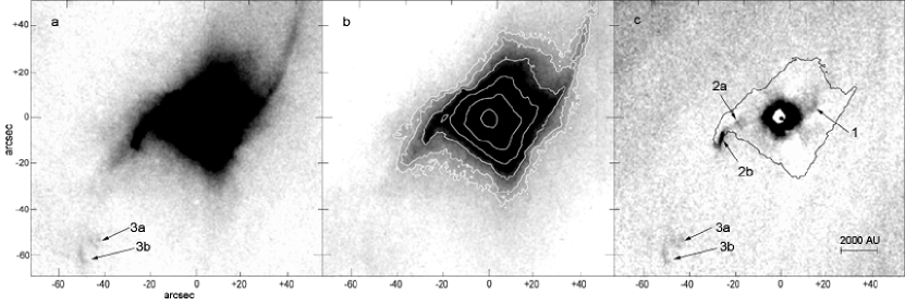
Figure 1: Narrowband Images of Elias 29. N is up and E is left in all panels. Offsets from RA(2000)= $16^{h}27^{m}09.43^{s}$ and Dec(2000)= $-24^{\circ}37^{\prime}18\farcs 7$ are indicated, in arcsec units. (a) Elias 29, observed through the narrowband H₂ filter with PANIC, (b) Elias 29 imaged with the Br$\gamma$ filter with PANIC, contour levels are 3, 5, 10, 20, 50, 500 $\sigma$. Note the absence of Features 3a and 3b in the Br$\gamma$ image, and their presence in the H₂ filter image. (c) Pure H₂ emission-line image of Elias 29, obtained by subtracting the scaled and aligned Br$\gamma$ filter image from the PANIC H₂ filter image with the Br$\gamma$ 10 $\sigma$ contour superimposed. The pure H₂ emission line features discussed in the text and listed in Table 1 are labelled.

References

- Arce & Sargent (2005) Arce, H. G. & Sargent, A.I. 2005, ApJ, 624, 232
- Allen & Burton (1993) Allen, D.A. & Burton, M.G. 1993, Nature, 363, 54
- Barsony et al. (1998) Barsony, M., Ward-Thompson, D., André, Ph., & O’Linger, J. 1998, ApJ, 509, 733
- Bence et al. (1996) Bence, S., RIcher, J.S., & Padman, R. 1996, MNRAS, 279, 886
- Bontemps et al. (1996) Bontemps, S., André, P., Terebey, S., & Cabrit, S. 1996, A&A, 311, 858
- Boogert et al. (2002) Boogert, A. C. A., Hogerheijde, M. R., Ceccarelli, C., Tielens, A. G. G. M., Van Dishoeck, E. F., Blake, G. A., Latter, W. B., & Motte, F. 2002, ApJ, 570, 708
- Davis et al. (2002) Davis, C.J., Stern, L., Ray, T.P., & Chrysostomou, A. 2002, A&A, 382, 1021
- Fridlund et al. (2005) Fridlund, C.V.M., Liseau, R., Djupvik, A.A., Huldtgren, M., White, G.J., Favata, F. & Giardino, G. 2005, A&A, 436, 983
- Ghez et al. (1993) Ghez, A., Neugebauer, G., & Matthews, K. 1993, AJ, 106, 2005
- Gómez et al. (2003) Gómez, M., Stark, D. P., Whitney, B. A., & Churchwell, E. 2003, AJ, 126, 863
- Gueth et al. (1996) Gueth, F., Guilloteau, S., & Bachiller, R. 1996, A&A, 307, 891
- Hartigan et al. (1994) Hartigan, P., Morse, J., & Raymond, J. 1994, ApJ, 436, 125
- Hodapp et al. (2005) Hodapp, K.W., Bally, J., Eislöffel, J., & Davis, C.J. 2005, AJ, 129, 1580
- Khanzadyan et al. (2004) Khanzadyan, T., Gredel, R., Smith, M. D., & Stanke, T. 2004, A&A, 426, 171
- Lai (2003) Lai, D. 2003, ApJL, 591, L119
- Lim (2001) Lim, A.J. 2001, MNRAS, 327, 507
- Liseau et al. (2005) Liseau, R., Fridlund, C.V.M., & Larsson, B. 2005, ApJ, 619, 959
- Martini et al. (2004) Martini, P., Persson, S.E., Murphy, D.C., Birk,C., Shectman, S.A., Gunnels, S.M., Koch, E. 2004, Proc. SPIE, 5492, 1653
- Masson & Chernin (1993) Masson, C.R. & Chernin, L. 1993, ApJ, 414, 230
- Mundt et al. (1990) Mundt, R., Bührke, T., Solf, J., Ray, T.P., & Raga, A.C. 1990, A&A, 232, 37
- Reipurth et al. (1997) Reipurth, B., Bally, J., & Devine, D. 1997, AJ, 114, 2708
- Romanova et al. (2006) Romanova, M.M., Ustyugova, G.V., Koldoba, A.V., & R.V.E. Lovelace 2006, ApJL, 635, L165
- Rosen & Smith (2004) Rosen, A., & Smith, M. D. 2004, MNRAS, 347, 1097
- Sahai et al. (2005) Sahai, R., Le Mignant, D., Sánchez Contreras, C., Campbell, R. D., & Chaffee, F. H. 2005, ApJL, 622, L53
- Sandell et al. (1999) Sandell, G. & 18 co-authors 1999, ApJ, 519, 236
- Schwartz & Greene (1999) Schwartz, R.D. & Greene, T. P. 1999, AJ, 117, 456
- Sekimoto et al. (1997) Sekimoto, Y., Tatematsu, K., Umemoto, T., Koyama, K., Tsuboi, Y., Hirano, N., & Yamamoto, S. 1991, ApJL, 489, L63
- Shull & Beckwith (1982) Shull, J.M. & Beckwith, S., ARAA, 20, 163
- Simon et al. (1987) Simon, M., Howell, R.R., Longmore, A.J., Wilking, B.A., Peterson, D.M., & Chen, W.P. 1987, ApJ, 320, 344
- Simon et al. (1995) Simon, M., Ghez, A.M., Leinert, Ch., Cassar, L., Chen, W.P., Howell, R.R., Jameson, R.F.m Matthews, K., Neugebauer, G., & Richichi, A. 1995, ApJ, 443, 625
- Smith & Rosen (2005) Smith M. D. & Rosen, A. 2005, MNRAS, 357, 579
- Stocke et al. (1988) Stocke, J., Hartigan, P.M., Strom, S.E., Strom, K.M., Anderson, E.R., Hartmann, L, & Kenyon, S.J. 1988, ApJS, 68, 229
- Terquem et al. (1999) Terquem, C., Eislöffel, J., Papaloizou, J., & Nelson, R.P. 1999, ApJL, 512, L131
- Whitney et al. (2003) Whitney, B.A., Wood, K., Bjorkman, J.E., & Cohen, M. 2003, ApJ, 598, 1079
- Wilson et al. (2003) Wilson, J.E., Eikenberry, S.S., Henderson, C.P., Hayward, T.L., Carson, J.C., Pirger, B., Barry, D.J., Brandl, B.R., Houck, J.R., Fitzgerald, G., & Stolberg, T.M. 2003, Proc. SPIE, 4841, 451
- Wolf-Chase et al. (2000) Wolf-Chase, G.A., Barsony, M., & O’Linger, J. 2000, AJ, 120, 1467
- Yamashita & Tamura (1992) Yamashita, T. & Tamura, M. 1992, ApJL, 387, L93
- Yun et al. (2001) Yun, J.C., Santos, C.A., Clemens, D.P., Afonso, J.M., McCaughrean, M.J., Preibisch, T., Stanke, T., & H. Zinnecker 2001, A&A, 372, L33