Concentration, Spin and Shape of Dark Matter Haloes: Scatter and the Dependence on Mass and Environment

Abstract

We use a series of cosmological N-body simulations for a flat $\Lambda$CDM cosmology to investigate the structural properties of dark matter haloes, at redshift zero, in the mass range $3\times 10^{9}h^{-1}\,\rm M_{\odot}\mathrel{\hbox to0.0pt{\lower 3.0pt\hbox{$\sim$}\hss}\raise 2.0pt\hbox{$<$}}M_{\rm vir}\mathrel{\hbox to0.0pt{\lower 3.0pt\hbox{$\sim$}\hss}\raise 2.0pt\hbox{$<$}}3\times 10^{13}$$h^{-1}\,\rm M_{\odot}$. These properties include the concentration parameter, $c$, the spin parameter, $\lambda$, and the mean axis ratio, $\bar{q}$. For the concentration-mass relation we find $c\propto M_{\rm vir}^{-0.11}$ in agreement with the model proposed by Bullock et al. (2001), but inconsistent with the alternative model of Eke, Navarro & Steinmetz (2001). The normalization of the concentration-mass relation, however, is 15 percent lower than suggested by Bullock et al. (2001). The results for $\lambda$ and $\bar{q}$ are in good agreement with previous studies, when extrapolated to the lower halo masses probed here, while $c$ and $\lambda$ are anti-correlated, in that high-spin haloes have, on average, lower concentrations. In an attempt to remove unrelaxed haloes from the sample, we compute for each halo the offset parameter, $x_{\rm off}$, defined as the distance between the most bound particle and the center of mass, in units of the virial radius. Removing haloes with large $x_{\rm off}$ increases the mean concentration by $\sim 10$ percent, lowers the mean spin parameter by $\sim 15$ percent, and removes the most prolate haloes. In addition, it largely removes the anti-correlation between $c$ and $\lambda$, though not entirely. We also investigate the relation between halo properties and their large-scale environment density. For low mass haloes we find that more concentrated haloes live in denser environments than their less concentrated counterparts of the same mass, consistent with recent correlation function analyses. Note, however, that the trend is weak compared to the scatter. For the halo spin parameters we find no environment dependence, while there is a weak indication that the most spherical haloes reside in slightly denser environments. Finally, using a simple model for disk galaxy formation we show that haloes that host low surface brightness galaxies are expected to be hosted by a biased sub-set of haloes. Not only do these haloes have spin parameters that are larger than average, they also have concentration parameters that are $\sim 15$ percent lower than the average at a given halo mass. We discuss the implications of all these findings for the claimed disagreement between halo concentrations inferred from LSB rotation curves, and those expected for a $\Lambda$CDM cosmology.

1 Introduction

The theory of cold dark matter (CDM) provides a successful framework for understanding structure formation in the universe. Within this paradigm dark matter collapses first into small haloes which merge to form progressively larger haloes over time. Galaxies are thought to form out of gas which cools and collapses to the centers of these dark matter haloes (White & Rees 1978).

In the standard picture of disk galaxy formation the structural and dynamical properties of disk galaxies are expected to be strongly related to the properties of the dark matter haloes in which they are embedded. In particular the characteristic sizes and rotation velocities of disk galaxies are determined (to first order) by the spin parameter, concentration parameter, and size of the host dark matter halo (e.g. Mo, Mao & White 1998, hereafter MMW). Consequently, the detailed rotation curve shapes of disk galaxies can, in principle, be used to constrain the structural properties of their dark matter haloes. This is especially true for low surface brightness (LSB) galaxies, which are believed to be dark matter dominated even at small radii. A steadily increasing data base of observed LSB rotation curves has resulted in a heated debate as to whether the slopes of the inner density profiles of dark matter dominated disk galaxies are consistent with the cuspy profiles found in N-body simulations, or similarly, whether the inferred concentrations are as high as predicted (see Swaters et al. 2003 and references therein).

Unfortunately, determining cusp slopes and/or concentration parameters from mass modeling rotation curves is non-unique, even for dark matter dominated galaxies (e.g., Dutton et al. 2005). In particular, determining $c$ requires knowledge of the virial radius, which is hard to constrain using data that only covers the inner $\simeq 10\%$ of the halo. As an alternative measure of the central density of a halo, Alam, Bullock & Weinberg (2002) introduced a dimensionless quantity that does not require knowledge of the halo virial radius, and demonstrated convincingly that the observed rotation curves of LSB galaxies imply halo concentrations that are systematically lower than predicted for a flat $\Lambda$CDM cosmology with a matter density $\Omega_{\rm M}=0.3$ and a scale-invariant Harrison-Zeldovich power-spectrum with normalization $\sigma_{8}=1.0$.

Further observational support for a lower normalization of the $c-M_{\rm vir}$ relation comes from the zero point of the rotation velocity-luminosity relation, also known as the Tully-Fisher relation (Tully & Fisher 1977) of disk galaxies (van den Bosch 2000). Detailed disk formation models have clearly demonstrated that the high concentrations of CDM haloes cause an overprediction of the rotation velocities at a fixed disk luminosity, at least for a ‘standard’ $\Lambda{\rm CDM}$ cosmology with $\Omega_{\rm M}=0.3$, $\Omega_{\rm\Lambda}=0.7$, and $\sigma_{8}=0.9$ (e.g., Dutton et al. 2007; Gnedin et al. 2006).

Although these discrepancies may indicate a genuine problem for the CDM paradigm, there are a number of alternative explanations: First of all, as shown by various authors (e.g. Swaters et al. 2003; Rhee et al. 2004; Spekkens, Giovanelli, & Haynes 2005) the observed rotation curves could be hampered by a variety of observational biases, such as beam smearing, slit offsets and inclination effects, all of which tend to underestimate the circular velocity in the central regions.

Secondly, the dark matter distribution could have been modified by astrophysical processes such as bars (e.g. Holley-Bockelmann, Weinberg, & Katz 2005) or dynamical friction (e.g. Mo & Mao 2004; Tonini et al. 2006). These processes tend to lower the concentration of the dark matter halo, bringing it in better agreement with the observations. On the other hand, adiabatic contraction (e.g., Blumenthal et al. 1986) thought to be associated with the formation of disk galaxies, actually tends to increase the halo concentration, and it remains to be seen whether the above mentioned processes are strong enough to undo this contraction and still cause a relative expansion of the inner halo (see Dutton et al. 2007 for a detailed discussion).

A third option is that the data-model comparison has been made for the wrong cosmology. In particular, a reduction in the power of cosmological density fluctuations on small scales causes a significant reduction of the predicted halo concentrations (e.g. Eke, Navarro & Steinmetz 2001; Zentner & Bullock 2002; Alam et al. 2002; van den Bosch, Mo, & Yang 2003). Most data-model comparisons have been based on a flat $\Lambda$CDM cosmology with $\Omega_{\rm M}=0.3$ and $\sigma_{8}=0.9$. However, recently the third year data release from the WMAP mission has advocated a model with $\Omega_{\rm M}\simeq 0.25$ and $\sigma_{8}\simeq 0.75$ (Spergel et al. 2006). This relatively small change in cosmological parameters causes a significant reduction of the predicted halo concentration parameters, bringing them in much better agreement with the data (e.g., Yang, Mo, & van den Bosch 2003; van den Bosch, Mo & Yang 2003).

Another potentially important cause for the discrepancy are systematic errors in the actual model predictions. Both Bullock et al. (2001a; hereafter B01) and Eke, Navarro & Steinmetz (2001; hereafter ENS) presented analytical models that allow one to compute the mean halo concentration for given halo mass, redshift and cosmology. Unfortunately, at redshift zero the predictions of these models are divergent below $\sim 10^{11}M_{\odot}$, with the ENS model predicting halo concentrations that are significantly lower. This is of particular importance for LSB (and dwarf) galaxies with $V\mathrel{\hbox to0.0pt{\lower 3.0pt\hbox{$\sim$}\hss}\raise 2.0pt\hbox{$<$}}100\,\rm km\,s^{-1}$, which are thought to typically reside in haloes with masses below this value. Both B01 and ENS calibrated their models against numerical simulations. Those of B01 probed the mass range between $3\times 10^{11}h^{-1}M_{\odot}$ and $6\times 10^{13}h^{-1}M_{\odot}$, while those of ENS probed an even narrower range from $3\times 10^{11}h^{-1}M_{\odot}$ to $3\times 10^{12}h^{-1}M_{\odot}$ (albeit with higher resolution). What is needed to discriminate between these models are simulations that resolve a large population of low mass haloes, which is one of the main objectives of this paper.

Another important issue that we wish to address in this paper is the possibility that the LSB disk galaxies that have been used to constrain halo concentrations reside in a biased sub-set of haloes (see discussion in Wechsler et al. 2006). Numerical simulations have shown that there is a significant scatter in both halo concentration, $c$, and halo spin parameter, $\lambda$, at a given halo mass (e.g. Bullock et al. 2001a,b). Thus if disk galaxies form in a biased subset of haloes, this could lead to an apparent discrepancy between theory and observation. In fact, there are a number of potential causes for such a bias. First of all, disk galaxies are expected to preferentially form in haloes that have not experienced any recent major merger. There is evidence that such a subset of haloes has higher mean $c$, lower mean $\lambda$, and lower scatter in both $c$ and $\lambda$ (Wechsler et al. 2002; D’Onghia & Burkert 2004). Clearly, this would worsen the disagreement between model and data. On the other hand, it has also been suggested that LSB galaxies preferentially reside in haloes with relatively low concentrations. First of all, since disks are thought to be in centrifugal equilibrium, less concentrated haloes will harbor less concentrated (i.e., lower surface brightness) disk galaxies (e.g., MMW, B01). In addition, using numerical simulations Bailin et al. (2005) found that haloes with higher spin parameters have, on average, lower concentration parameters. Since LSB galaxies are thought to be those with high spin parameters such a correlation would imply that LSB galaxies reside in haloes with relatively low concentrations. If confirmed this could offer an alternative explanation as to why (some) LSB galaxies have lower concentrations than predicted. Note, however, that previous studies (B01, Navarro, Frenk & White 1997, hereafter NFW), have found no correlation between spin parameter and concentration.

Another potential bias for disk galaxy formation could arise if there is a correlation between environment (defined as the large scale matter density) and $c$ or $\lambda$. In particular, Harker et al. (2006) found evidence that low mass haloes in dense environments assemble earlier than haloes of the same mass in under-dense environments. Note however, that for the lowest density environments this trend reverses so that formation redshifts actually increase with decreasing density. Since haloes that assemble later are less concentrated (Wechsler et al. 2002), one thus may expect a similar correlation between halo concentration and environmental density. If dwarf and LSB galaxies preferentially form in under-dense regions this could also help explain the lower than expected halo concentrations of these galaxies.

In this paper we study galaxy size dark matter haloes from a set of cosmological N-body simulations with the following goals: (i) to test the predictions of B01 and ENS regarding the halo concentrations of low mass haloes (down to $\sim 3\times 10^{9}h^{-1}M_{\odot}$), (ii) to determine the scatter in concentration, spin parameter, and halo shape at a given mass, (iii) to determine whether there is a correlation between the spin and concentration parameters, and (iv) to determine whether $c$, $\lambda$ and halo shape depend on the density of the environment in which the halo is located. Our paper is organized as follows. Section 2 describes our set of N-body simulations. In Section 3 we discuss how halo concentration, halo spin parameter and halo shape depend on halo mass. Sections 4 investigates whether $c$ and $\lambda$ are correlated, while Section 5 focuses on the environment dependence of halo properties. In Section 6 we use simple models for disk formation to investigate whether one expects LSB galaxies to reside in haloes with a biased concentration parameter. Finally, we summarize our results in Section 7.

2 N-body simulations

In order to explore as wide a range of virial masses as possible, we run simulations of 4 different box sizes, listed in Table 1. For comparison we also show the parameters of the Bullock et al. (2001a,b), Bailin et al. (2005) and millennium run (Springel et al. 2005) simulations. The B01 simulation has similar size and mass resolution as our 64_a,b boxes, while our smallest box simulation has a mass resolution that is $\sim 5$ times higher than that of Bailin et al. (2005). In order to test for cosmic variance, and to increase the size of our sample we ran two simulations for each of the three smallest box sizes.

All simulations have been performed with PKDGRAV, a tree code written by Joachim Stadel and Thomas Quinn (Stadel 2001). The code uses spline kernel softening, for which the forces become completely Newtonian at 2 softening lengths. Individual time steps for each particle are chosen proportional to the square root of the softening length, $\epsilon$, over the acceleration, $a$: $\Delta t_{i}=\eta\sqrt{\epsilon/a_{i}}$. Throughout, we set $\eta=0.2$, and we keep the value of the softening length constant in comoving coordinates during each run. The physical values of $\epsilon$ at $z=0$ are listed in Table 1. Forces are computed using terms up to hexadecapole order and a node-opening angle $\theta$ which we change from $0.55$ initially to $0.7$ at $z=2$. This allows a higher force accuracy when the mass distribution is nearly smooth and the relative force errors can be large.

We adopt a flat $\Lambda$CDM cosmology with parameters from the first year WMAP results (Spergel et al. 2003): matter density $\Omega_{\rm M}=0.268$, baryon density $\Omega_{b}=0.044$, Hubble constant $h\equiv H_{0}/(100\>{\rm km}\,{\rm s}^{-1}\,{\rm Mpc}^{-1})=0.71$, and a scale-invariant, Harrison-Zeldovich power-spectrum with normalization $\sigma_{8}=0.9$. The initial conditions are generated with the GRAFIC2 package (Bertschinger 2001), which also computes the transfer function as described in Ma & Bertschinger (1995). The starting redshifts $z_{i}$ are set to the time when the standard deviation of the smallest density fluctuations resolved within the simulation box reaches $0.2$ (the smallest scale resolved within the initial conditions is defined as twice the intra-particle distance, while the maximum scale is set by the Box size).

Table 1: N-body Simulation Parameters

Name	Box size	N	particle mass	force soft.
	$[h^{-1}{\rm Mpc}]$		$[h^{-1}M_{\odot}]$	$[h^{-1}{\rm kpc}]$
14a, 14b	14.2	$250^{3}$	$1.4\times 10^{7}$	0.43
28a, 28b	28.4	$250^{3}$	$1.1\times 10^{8}$	0.85
64a, 64b	63.9	$300^{3}$	$7.2\times 10^{8}$	1.92
128	127.8	$300^{3}$	$5.8\times 10^{9}$	3.83
Bullock	60	$256^{3}$	$1.1\times 10^{9}$	1.8
Bailin	50	$512^{3}$	$7.8\times 10^{7}$	5.0
Millennium	500	$2160^{3}$	$8.6\times 10^{8}$	5.0

In all of our numerical simulations, haloes are identified using a SO (Spherical Overdensity) algorithm. As a first step, candidate haloes are located using the standard friends-of-friends (FOF) algorithm, with a linking length $bn^{-1/3}$, with $n$ the mean particle density and $b$ a free parameter which we set to $0.2$. We only keep FOF haloes with at least $N_{\rm min}=200$ particles, which we subject to the following two operations: (i) we find the point, $C$, where the gravitational potential due to the group of particles is minimum, and (ii) we determine the radius $R_{\rm vir}$, centered on $C$, inside of which the density contrast is $\Delta_{\rm vir}$. For our adopted cosmology $\Delta_{\rm vir}\simeq 98$ (using the fitting function of Mainini et al. 2003). Using all particles in the corresponding sphere we iterate the above procedure until we converge onto a stable particle set. The set is discarded if, at some stage, the sphere contains less than $N_{\rm min}$ particles. If a particle is a potential member of two haloes it is assigned to the more massive one. For each stable particle set we obtain the virial radius, $R_{\rm vir}$, the number of particles within the virial radius, $N_{\rm vir}$, and the virial mass, $M_{\rm vir}$. Above a mass threshold of $N_{\rm vir}=250$ particles there are $\sim 2750$, $3750$, $7450$ and $4500$ haloes in the simulations of box size 14.2, 28.4, 63.9, 127.8 $h^{-1}{\rm Mpc}$ respectively (these numbers refer to the two versions of each box size combined together).

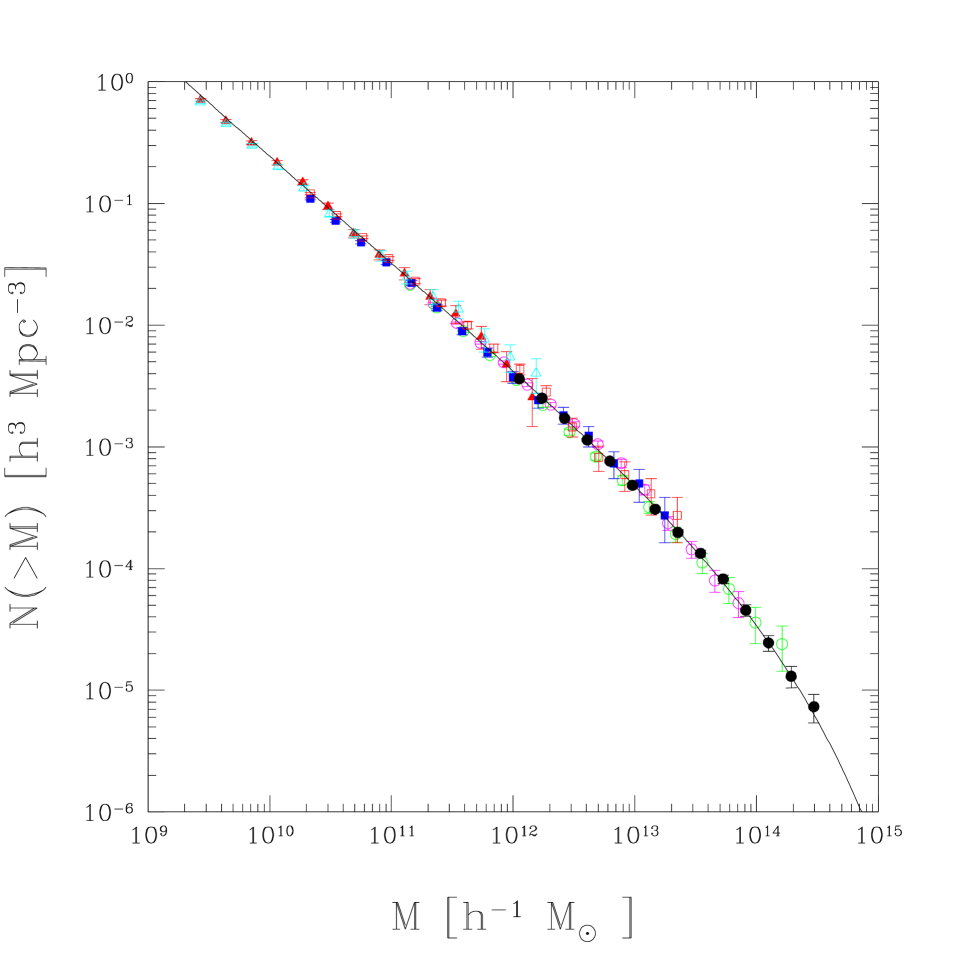
Figure 1: Mass functions for the simulations. The point and color types correspond to the different runs: 14a (cyan triangles); 14b (red triangles); 28a (blue squares); 28b (yellow squares); 64a (magenta open circles); 64b (green open circles); 128 (black circles). The solid line is the Sheth & Tormen prediction for $\sigma_{8}=0.9$.

In Fig.  1 we report the comparison of the halo mass functions of all our simulations with the analytical mass function of Sheth & Tormen (2002). Since the Sheth & Tormen mass function has been tuned to reproduce the mass function of FOF haloes (with $b=0.2$), we use the same FOF masses here. For the remainder of this paper, however, we consistently will use the spherical overdensity masses, $M_{\rm vir}$, described above. Note that the FOF mass functions agree well with the Sheth & Tormen mass function over the full five orders of magnitude in halo mass probed by our simulations: all data points are consistent with the model within one sigma (error bars show the Poisson noise in each bin due to the finite number of haloes). Moreover all the simulations made with different box sizes agree with each other in the mass ranges where they overlap.

2.1 Halo parameters

For each halo we determine a set of parameters as described below. All of these parameters are derived from the SO haloes (i.e. from the particle sets defined by the SO criteria), rather than from the FOF particle sets.

2.1.1 concentration parameter

N-body simulations have shown that the spherically averaged density profiles of DM haloes can be well described by a two parameter NFW profile:

$$\frac{\rho(r)}{\rho_{\rm crit}}=\frac{\delta_{\rm c}}{(r/r_{\rm s})(1+r/r_{\rm s})^{2}},$$ (1)

where $\rho_{\rm crit}$ is the critical density of the universe, $\delta_{\rm c}$ is the characteristic overdensity of the halo, and $r_{\rm s}$ is the radius where the logarithmic slope of the halo density profile ${\rm d}\ln\rho/{\rm d}\ln r=-2$ (NFW). A more useful parametrization is in terms of the virial mass, $M_{\rm vir}$, and concentration parameter, $c\equiv R_{\rm vir}/r_{\rm s}$. The virial mass and radius are related by $M_{\rm vir}=\Delta_{\rm vir}\rho_{\rm crit}(4\pi/3)R_{\rm vir}^{3}$, where $\Delta_{\rm vir}$ is the density contrast of the halo.

To compute the concentration of a halo we first determine its density profile. The halo center is defined as the location of the most bound halo particle, and we compute the density ($\rho_{i}$) in 50 spherical shells, spaced equally in log radius. Errors on the density are computed from the Poisson noise due to the finite number of particles in each mass shell. The resulting density profile is fit with a NFW profile (Eq. 1), which provides a good fit to most haloes over the range of radii we are interested in. Note that, in this paper, we are not concerned with the inner asymptotic slope of the density profile. During the fitting procedure we treat both $r_{\rm s}$ and $\delta_{c}$ as free parameters. Their values, and associated uncertainties, are obtained via a $\chi^{2}$ minimization procedure using the Levenberg & Marquart method. We define the r.m.s. of the fit as:

$$\rho_{\rm rms}=\frac{1}{N}\sum_{i}^{N}{(\ln\rho_{i}-\ln\rho_{m})^{2}}$$ (2)

where $\rho_{\rm m}$ is the fitted NFW density distribution. We do not use the $\chi^{2}$ value of the best-fit since this increases with $N_{\rm vir}$. This occurs because higher resolution haloes have better resolved substructure and smaller Poisson errors on the density, thus making the fit worse. Finally, we compute the concentration of the halo, $c$, using the virial radius obtained from the SO algorithm, and we define the error on $\log c$ as $(\sigma_{r_{\rm s}}/r_{\rm s})/\ln(10)$, where $\sigma_{r_{\rm s}}$ is the fitting uncertainty on $r_{\rm s}$.

We checked our concentration fit pipeline against the one suggested by B01. As a test we used both the procedures to compute $c$ in all our cubes. No systematic offset arises in the concentration vs. mass relation due to the different halo definition and fitting procedure.

2.1.2 spin parameter

The spin parameter is a dimensionless measure of the amount of rotation of a dark matter halo. The standard definition of the spin parameter, due to Peebles (1969), is given by

$${\lambda=\frac{J_{\rm vir}|E_{\rm vir}|^{1/2}}{GM_{\rm vir}^{5/2}},}$$ (3)

where $M_{\rm vir},$ $J_{\rm vir}$ and $E_{\rm vir}$ are the mass, total angular momentum and energy of the halo, respectively. Due to difficulties with accurately measuring $E_{\rm vir}$, Bullock et al. (2001b) introduced a modified spin parameter:

$$\lambda^{\prime}=\frac{J_{\rm vir}}{\sqrt{2}M_{\rm vir}V_{\rm vir}R_{\rm vir}}$$ (4)

with $V_{\rm vir}$ the circular velocity at the virial radius. For a singular isothermal sphere these two definitions are equivalent. For a pure NFW halo, however, they are related according to $\lambda=\lambda^{\prime}f(c)^{1/2}$ with $f(c)=\frac{1}{2}c[(1+c)^{2}-1-2(1+c)\ln(1+c)]/[c-(1+c)\ln(1+c)]^{2}$ (MMW). In what follows, we define $\lambda^{\prime}_{\rm c}\equiv\lambda^{\prime}f(c)$ as the “corrected” spin parameter.

In order to avoid potential problems and inaccuracies with the measurement of $E_{\rm vir}$, we adopt the $\lambda^{\prime}$ definition for the halo spin parameter, unless specifically stated otherwise. The advantage of $\lambda^{\prime}$ over $\lambda^{\prime}_{\rm c}$ is that the latter can introduce artificial correlations between halo concentration and halo spin parameter, since an error in $c$ translates into an error in $f(c)$ and hence $\lambda^{\prime}_{\rm c}$. We define the uncertainty in $\log\lambda^{\prime}$ as $(\sigma_{J}/J)/\ln(10)$, were we use that $\sigma_{J}/J=\sqrt{\frac{1}{N}(1+0.04/\lambda^{\prime 2})}\simeq 0.2/\lambda^{\prime}\sqrt{(}N)$ (Bullock et al. 2001b). Note that this implies that the errors on $\lambda^{\prime}$ are largest for haloes with a low spin parameter and with few particles.

2.1.3 shape parameter

Determining the shape of a three-dimensional distribution of particles is a non-trivial task (i.e. Jing & Suto 2002). Following Allgood et al. (2006) we determine the shape of our haloes starting from the inertia tensor. As a first step the inertia tensor of the halo is computed using all the particles within the virial radius; in this way we obtain a $3\times 3$ matrix. Then the inertia tensor is diagonalized and the particle distribution is rotated according to the eigen vectors. In this new frame (in which the moment of inertia tensor is diagonal) the ratios $a_{2}/a_{1}$ and $a_{3}/a_{1}$ ($a_{1},a_{2},a_{3}$ being the major, intermediate and minor axis, respectively) are given by:

$${a_{2}\over a_{1}}=\sqrt{{\sum m_{i}y_{i}^{2}}\over\sum{m_{i}x_{i}^{2}}},\newline {a_{3}\over a_{1}}=\sqrt{{\sum m_{i}z_{i}^{2}}\over\sum{m_{i}x_{i}^{2}}}.$$ (5)

Next we again compute the inertia tensor, but this time only using the particles inside the ellipsoid defined by $a_{1}$, $a_{2}$ and $a_{3}$. When deforming the ellipsoidal volume of the halo, we keep the longest axis ($a_{1}$) equal to the original radius of the spherical volume (cf. Allgood et al. 2006). We iterate this procedure until we converge to a stable set of the axis ratios.

Since dark matter haloes tend to be prolate, a useful parameter that describes the shape of the halo is $\bar{q}\equiv(a_{2}+a_{3})/2a_{1}$, with the limiting cases being a sphere ($\bar{q}=1$) and a needle ($\bar{q}=0$).

2.1.4 offset parameter

The last quantity that we compute for each halo is the offset, $x_{\rm off}$, defined as the distance between the most bound particle (used as the center for the density profile) and the center of mass of the halo, in units of the virial radius. This offset is a measure for the extent to which the halo is relaxed: relaxed haloes in equilibrium will have a smooth, radially symmetric density distribution, and thus an offset that is virtually equal to zero. Unrelaxed haloes, such as those that have only recently experienced a major merger, are likely to reveal a strongly asymmetric mass distribution, and thus a relatively large $x_{\rm off}$. Although some unrelaxed haloes may have a small $x_{\rm off}$, the advantage of this parameter over, for example, the actual virial ratio, $2T/V$, as a function of radius (Macciò, Murante & Bonometto 2003; Shaw et al. 2006), is that the former is trivial to evaluate.

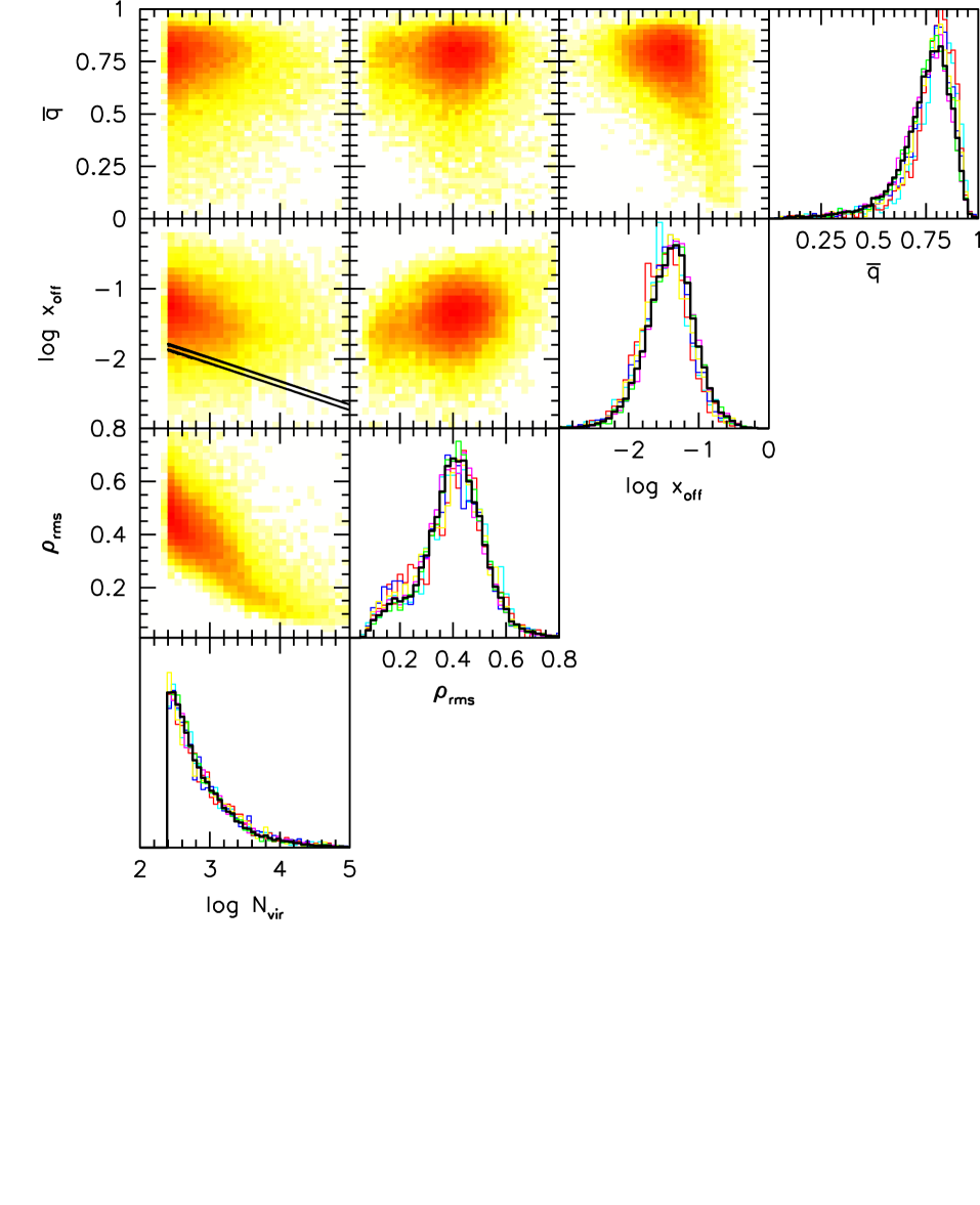
Figure 2: Correlations between, $N_{\rm vir}$, $\rho_{\rm rms}$, $x_{\rm off}$, and $\bar{q}$. The color coding in the density plots is according to the logarithm of the number of points in each cell. For the histograms the colors correspond to the different simulations as in Fig. 1, the thick black line shows the histograms of the combined samples. The black lines in the $x_{\rm off}-N_{\rm vir}$ plot shows the ratio of the softening length to the virial radius.

Fig. 2 shows histograms of, and correlations between $N_{\rm vir}$, $\rho_{\rm rms}$, $x_{\rm off}$, and $\bar{q}$. The rms of the density profile fit decreases with $N_{\rm vir}$, as expected, while $x_{\rm off}$ and $\bar{q}$ are uncorrelated with $N_{\rm vir}$ (especially for $N_{\rm vir}>10^{3})$. The solid lines in the $x_{\rm off}$-$N_{\rm vir}$ plot show the ratios of the softening length to the virial radius. This shows that the offset parameter is not effected by resolution effects. In an ideal halo simulation with a large number of particles $x_{\rm off}$ is expected to decrease with the decrease of the halo mass. We do not see this trend in the $x_{\rm off}$-$N_{\rm vir}$ relation because in our simulations the value of $x_{\rm off}$ is mostly dominated by numerical effects at the low mass tail. Moreover since we used different simulations with different mass resolution there is not a one to one relation between mass and $N_{\rm vir}$. Note also that $x_{\rm off}$ is uncorrelated with $\rho_{\rm rms}$, but that there is a strong correlation between $x_{\rm off}$ and $\bar{q}$ so that more prolate haloes tend to have larger offsets. We discuss the implications of this correlation in §3.1.

The distributions of $\rho_{\rm rms}$ and $\log(x_{\rm off})$ are approximately normal with means of $0.4$ and $-1.4$, respectively. The distribution of $\bar{q}$, on the other hand, is strongly skewed. Note also that the $\bar{q}$-distributions are slightly different for different box-sizes. This is because there is a correlation between halo mass and halo shape, such that more massive haloes are less spherical (see Section 3.1 below). Since larger boxes contain more massive haloes, this results in lower mean axis ratios.

3 Mass dependence of Spin, Concentration and Shape

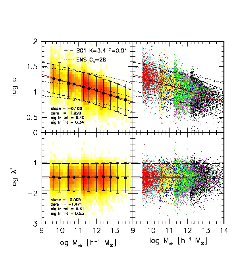
Figure 3: Relations between concentration, spin parameter and virial mass for haloes with $N_{\rm vir}>250$. The dashed lines give the mean and $2\sigma$ scatter from Bullock et al. 2001a,b. Dotted lines give the ENS model prediction. The solid red lines give weighted power-law fits: $y={\rm zero}+{\rm slope}(\log M_{\rm vir}-12)$, where $y=\log c$ or $\log\lambda$ and $M_{\rm vir}$ is in units of $h^{-1}M_{\odot}$. The parameters of the fits are given in the lower left corner of each panel. The panels on the left show the data binned in mass. The filled circles give the error weighted mean, the small error bars gives the Poisson error on the mean while the larger error bars give the intrinsic 2-sigma scatter. The panels on the right show all the data points color coded according to the simulation: 14a (cyan); 14b (red); 28a (blue); 28b (yellow); 64a (magenta); 64b (green); 128 (black).

Fig. 3 shows the relations of concentration vs. mass, and spin parameter vs. mass for all haloes with more than 250 particles within the virial radius. The right panels show the data from the simulations with the four box sizes clearly visible. The left panels show the mean (solid dots) and twice the standard deviation of $c$ and $\lambda^{\prime}$ (error bars) in bins equally spaced in $\log M_{\rm vir}$ (plotted at the mean $M_{\rm vir}$ in each bin). The mean $c$ and $\lambda^{\prime}$ are computed taking account of both the estimated measurement errors and the intrinsic scatter, using

$$\bar{y}=\frac{\Sigma_{i}y_{i}w_{i}}{\Sigma_{i}w_{i}},\;\;w_{i}=(\sigma_{\rm int}^{2}+\sigma_{i}^{2})^{-1}$$ (6)

Here $y_{i}$ denotes either $c$ or $\lambda^{\prime}$ of the $i$th halo, $w_{i}$ is the weight (haloes with larger uncertainties receive less weight), and $\sigma_{i}$ is the measurement error on $c$ or $\lambda^{\prime}$. The intrinsic scatter $\sigma_{\rm int}$ is given by

$$\sigma_{\rm int}^{2}=\frac{\Sigma_{i}\left[(y_{i}-\bar{y})^{2}-\sigma_{i}^{2}\right]w_{i}}{\Sigma_{i}w_{i}}.$$ (7)

Since these two equations are coupled the computation of $\bar{y}$ and $\sigma_{\rm int}$ requires an iterative procedure. We start by computing $\bar{y}$ and $\sigma_{\rm int}$ with $w_{i}=1$. Next we iterate until a stable solution for $\bar{y}$ and $\sigma_{\rm int}$ is found. This procedure converges rapidly, typically in 3-4 iterations.

The solid red lines in Fig. 3 show weighted (using errors on $c$ and $\lambda^{\prime}$) least squares fits of $c$ and $\lambda^{\prime}$ on $M_{\rm vir}$. The $c-M_{\rm vir}$ relation is well fitted by a single power-law over four orders of magnitude in mass $3\times 10^{9}\,h^{-1}\,\rm M_{\odot}\mathrel{\hbox to0.0pt{\lower 3.0pt\hbox{$\sim$}\hss}\raise 2.0pt\hbox{$<$}}M_{\rm vir}\mathrel{\hbox to0.0pt{\lower 3.0pt\hbox{$\sim$}\hss}\raise 2.0pt\hbox{$<$}}3\times 10^{13}\,h^{-1}\,\rm M_{\odot}$, with

$$\log c=1.020[\pm 0.015]-0.109[\pm 0.005](\log M_{\rm vir}-12).$$ (8)

Note that $M_{\rm vir}$ is in units of $h^{-1}M_{\odot}$. The numbers in square brackets give the scatter in the corresponding value between the seven different simulations. The total scatter about this mean relation is $\sigma_{\ln c}=0.40\pm 0.03$ and the intrinsic scatter is $\sigma_{\ln c}=0.33\pm 0.03$, where again the uncertainty corresponds to the box-to-box scatter. These are in excellent agreement with the total and intrinsic scatter found by B01 which are $0.41$ and $0.32$, respectively (see also Wechsler et al. 2002). The slope of the $\lambda^{\prime}-M_{\rm vir}$ relation is consistent with zero, in agreement with previous studies (e.g. Lemson & Kauffmann 1999, hereafter LK99; Shaw et al. 2006). If we take $\lambda^{\prime}$ to be independent of $M_{\rm vir}$, we find a median $\lambda^{\prime}=0.034\pm 0.001$ with an intrinsic scatter of $\sigma_{\ln\lambda^{\prime}}=0.55\pm 0.01$, which are in excellent agreement with Bullock et al. (2001b) (median of $\lambda^{\prime}=0.035\pm 0.005$ and $\sigma_{\ln\lambda^{\prime}}=0.50\pm 0.03$) and other studies (e.g., van den Bosch et al. 2002; Avila-Reese et al. 2005).

The dashed and dotted lines show the mean $c(M_{\rm vir})$ for the B01 and ENS models, respectively. In addition, for both models we also show the upper and lower $2\sigma$ intrinsic scatter bounds, where we adopt $\sigma_{\ln c}=0.32$ (Wechsler et al. 2002). The B01 model has two free parameters: $K$, which determines the normalization of the relation, and $F$, which effects the slope. The ENS model has just one free parameter $C_{\sigma}$ which controls the normalization; the slope is fully determined by the model. If we adopt $F=0.01$, as advocated by B01, we find that the slope of the B01 model is in excellent agreement with our simulations over the full range of masses covered. Consequently, our data is inconsistent with the significantly shallower slope of the ENS model. Note that ENS compared their model to a very small sample of relaxed haloes ($\sim 15$), albeit with high resolution ($N_{\rm vir}>30000$), over a small mass range $M_{\rm vir}\simeq 2\times 10^{11}-4\times 10^{12}\;h^{-1}\,\rm M_{\odot}$. Over this mass range the ENS model is in reasonable agreement with our simulation data.

In terms of the normalization our data is best fit with $K=3.4\pm 0.1$ (for $F=0.01$), where the error reflects the effect of cosmic variance as determined from the various independent simulation boxes. This is 15 percent lower than the $K=4.0$ originally advocated by B01, but consistent with Zhao et al. (2003) and Kuhlen et al. (2005), who found $K=3.5$ (both for $F=0.01$). In their paper Kuhlen et al. argued that the cause for their lower normalization might be due to the $N$-body code used for their simulations (GADGET-1). However, we have used an independent code, PKDGRAV, and obtain the same result. We therefore suspect that the cause for this discrepancy resides somewhere else. Indeed, as it turns out, B01 used a slightly different transfer function for setting up the initial conditions of their numerical simulation than for computing their model. If they correct this, they obtain a best fit $K=3.75$ (James Bullock & Andrew Zentner, private communication). If we take our (admittedly crude) estimate for the cosmic variance at face value, this still implies that we predict a normalization that is significantly lower (at the $3\sigma$ level).

As pointed out by B01, a better match to the slope of the $c-M_{\rm vir}$ relation for haloes more massive than $\simeq 10^{13}h^{-1}\,\rm M_{\odot}$ (at the expense of worsening the agreement for haloes with $M\mathrel{\hbox to0.0pt{\lower 3.0pt\hbox{$\sim$}\hss}\raise 2.0pt\hbox{$<$}}10^{11}h^{-1}\,\rm M_{\odot}$) can be obtained by using $F=0.001$, in which case we find that $K=2.6$. This is again approximately 15 percent smaller than the $K=3.0$ advocated by B01 for this value of $F$.

3.1 The Impact of Unrelaxed Haloes

Our halo finder (and halo finders in general) do not distinguish between relaxed and unrelaxed haloes. There are two reasons why we might want to remove unrelaxed halos. First, and most importantly, unrelaxed haloes often have poorly defined centers, which makes the determination of a radial density profile, and hence of the concentration parameter, an ill-defined problem. Secondly for applications to disk galaxy formation, haloes that are not in dynamical equilibrium are unlikely to host disk galaxies, and even less likely to host the more dynamically fragile LSB galaxies. In this case, the halo parameters inferred from (LSB) disk rotation curves need to be compared to those of the subset of relaxed haloes only.

One could imagine using $\rho_{\rm rms}$ (the r.m.s. of the NFW fit to the density profile) to decide whether a halo is relaxed or not. However, while it is true that $\rho_{\rm rms}$ is typically high for unrelaxed haloes, haloes with relatively few particles also have a high $\rho_{\rm rms}$ (due to Poisson noise) even when they are relaxed. This is evident from Fig. 2, which shows that $\rho_{\rm rms}$ and $N_{\rm vir}$ are strongly correlated. Furthermore not all unrelaxed haloes have a high $\rho_{\rm rms}$. We found several examples of haloes with low $\rho_{\rm rms}$ which are clearly unrelaxed. This is due to the smoothing effects of spherical averaging when computing the density profile. However, these haloes are often characterized by a large $x_{\rm off}$ (the offset between the most bound particle and the center of mass). In what follows we therefore use both $\rho_{\rm rms}$ and $x_{\rm off}$ to judge whether a halo is relaxed or not.

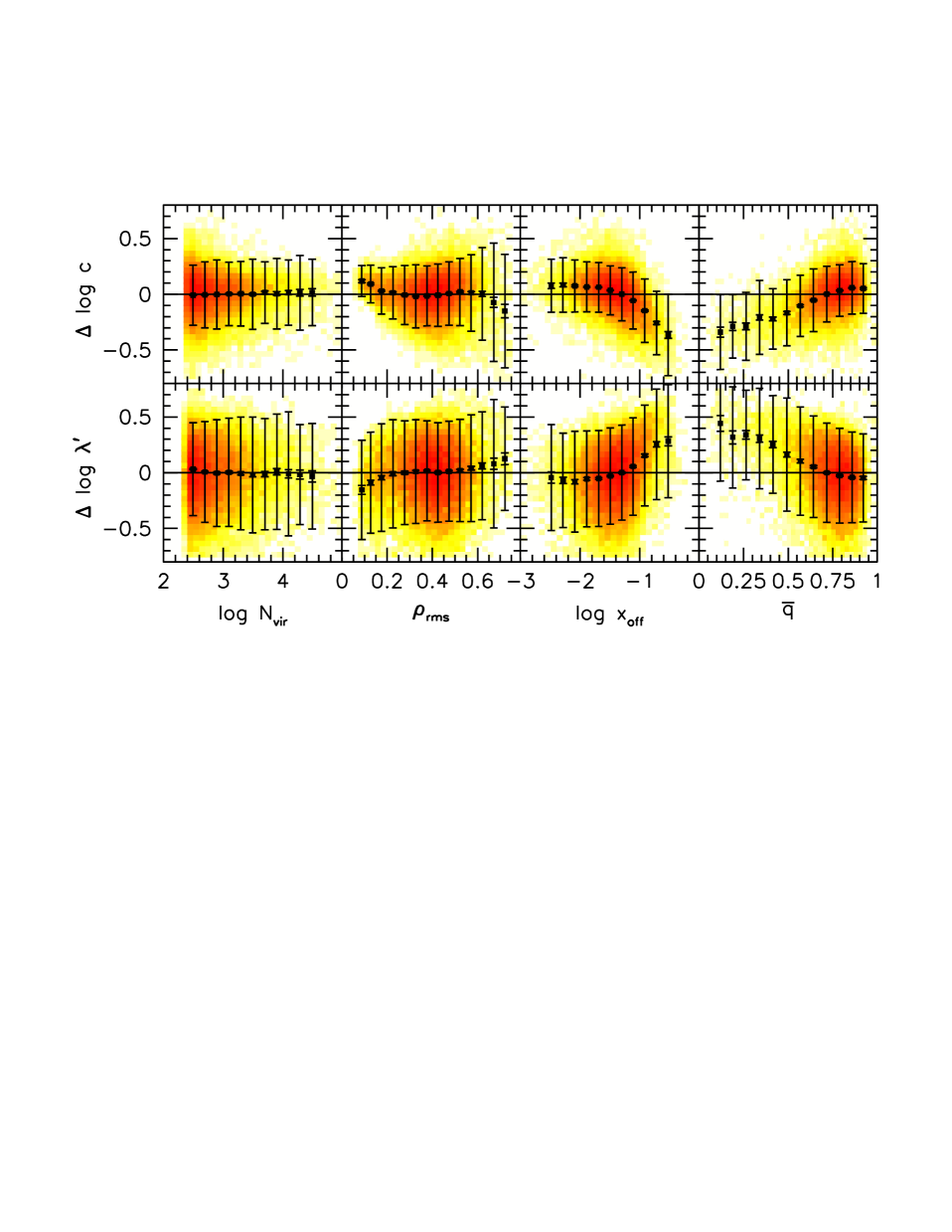
Figure 4: Residuals of the $c-M_{\rm vir}$ (upper panels) and $\lambda^{\prime}-M_{\rm vir}$ (lower panels) relations as fitted in Fig. 3, against $N_{\rm vir}$, $\rho_{\rm rms}$, $x_{\rm off}$, and $\bar{q}$ for all haloes with $N_{\rm vir}>250$. The large error bars show twice the $1\sigma$ intrinsic scatter, while the small error bar shows the possion error on the mean.

Fig. 4 shows the residuals of the $c-M_{\rm vir}$ and $\lambda^{\prime}-M_{\rm vir}$ relations for haloes with $N_{\rm vir}>250$, against $N_{\rm vir}$, $\rho_{\rm rms}$, $x_{\rm off}$, and $\bar{q}$. The filled circles and error bars show the mean and 2$\sigma$ scatter of points in equally spaced bins. The smaller error bars, sometimes barely visible, show the Poisson error on the mean ($\sigma/\sqrt{N}$). Both the $c$ and $\lambda^{\prime}$ residuals show no trend with $N_{\rm vir}$, even down to our limit of 250 particles. This indicates that numerical resolution is not affecting our results.

Table 2: Effect of RMS parameter on $c$ and $\lambda^{\prime}$ distributions for haloes with $N_{\rm vir}>10000$.

$\rho_{\rm rms}$	N haloes	$<\log c_{12}>$	$\sigma_{\ln c}$	$<\log\lambda^{\prime}>$	$\sigma_{\ln\lambda^{\prime}}$	$<\rho_{\rm rms}>$	$<x_{\rm off}>$	$<\bar{q}>$
$>$ 0.25	88	0.770	0.392	-1.285	0.528	0.36	0.100	0.52
0.15-0.25	183	0.986	0.281	-1.436	0.596	0.19	0.038	0.66
0.10-0.15	226	1.111	0.204	-1.552	0.513	0.12	0.022	0.73
0.00-0.10	117	1.138	0.167	-1.625	0.516	0.09	0.018	0.74
$>$ 0.0	614	1.039	0.353	-1.493	0.597	0.17	0.031	0.68

Interestingly we find that haloes with the lowest $\rho_{\rm rms}$ tend to have larger $c$, smaller scatter in $c$, and lower $\lambda^{\prime}$. A similar result for halo $c$ was found by Jing (2000), who used the maximum deviation of the density profile from the NFW fit, which is similar to our $\rho_{\rm rms}$ parameter. In Table 2 we show the effect of the RMS parameter on the mean and scatter of halo $c$ and $\lambda^{\prime}$. Here $<\log c_{12}>$ is the zero point of the $c-M_{\rm vir}$ relation, measured at $M_{\rm vir}=10^{12}h^{-1}\,\rm M_{\odot}$. To allow for comparison with Jing (2000) we only use haloes with $N_{\rm vir}>10000$. We find that the highest $\rho_{\rm rms}$ haloes have a mean $c$ which is roughly a factor of 2 lower, and a scatter in $c$ which is roughly a factor of 2 higher, than the lowest $\rho_{\rm rms}$ haloes, in agreement with Jing (2000). Additionally we also find a factor of 2 difference between the average $\lambda^{\prime}$ of the highest and lowest $\rho_{\rm rms}$ haloes. Haloes with the highest $\rho_{\rm rms}$ have the highest mean offset parameter, $<x_{\rm off}>$, and the lowest mean halo shape parameter, $<\bar{q}>$. This suggests that these haloes are the most unrelaxed.

The trends between $c$ and $\lambda^{\prime}$ with $x_{\rm off}$ are shown in the third column of Fig. 4. These show that for haloes with small $x_{\rm off}$ the residuals are uncorrelated with $x_{\rm off}$. However, these haloes have concentrations that are higher and spin parameters that are lower than the overall average. For $x_{\rm off}\mathrel{\hbox to0.0pt{\lower 3.0pt\hbox{$\sim$}\hss}\raise 2.0pt\hbox{$>$}}0.04$ ($\log x_{\rm off}>-1.4$) there is a clear systematic trend that haloes with larger $x_{\rm off}$ have lower $c$ and higher $\lambda^{\prime}$. The same trends are seen for $\bar{q}$, where more prolate haloes (of a given mass) have lower $c$ and higher $\lambda^{\prime}$. This basically reflects the correlation between $x_{\rm off}$ and $\bar{q}$ (see Fig. 2).

These trends are consistent with unrelaxed haloes being the systems that experienced a recent major merger: (i) the center of the halo is poorly defined, which results in a large $x_{\rm off}$ and an artificially shallow (low concentration) density profile, (ii) the halo shape is more prolate, and (iii) the spin parameter is higher due to the orbital angular momentum ‘transferred’ to the system due to the merger (e.g., Vitvitska et al. 2002; Maller, Dekel & Somerville 2002). Ideally one would test the correspondence between merger histories and $x_{\rm off}$ using the actual merger trees extracted from the simulation. Unfortunately, we did not store sufficient outputs to be able to do so. We intend to address these issues in a future paper, based on a new set of simulations.

We now split our sample into 4 sub-samples according to $\rho_{\rm rms}$ and $x_{\rm off}$, with dividers of $\rho_{\rm rms}=0.4$ and $x_{\rm off}=0.04$, which correspond to the mean of the distributions of $\rho_{\rm rms}$ and $x_{\rm off}$, respectively (see Fig. 2). We refer to the 4-subsamples as:

• GOOD  ($\rho_{\rm rms}<0.4$ & $x_{\rm off}<0.04$);

• BAD     ($\rho_{\rm rms}<0.4$ & $x_{\rm off}>0.04$);

• UGLY   ($\rho_{\rm rms}>0.4$ & $x_{\rm off}>0.04$);

• NOISY ($\rho_{\rm rms}>0.4$ & $x_{\rm off}<0.04$).

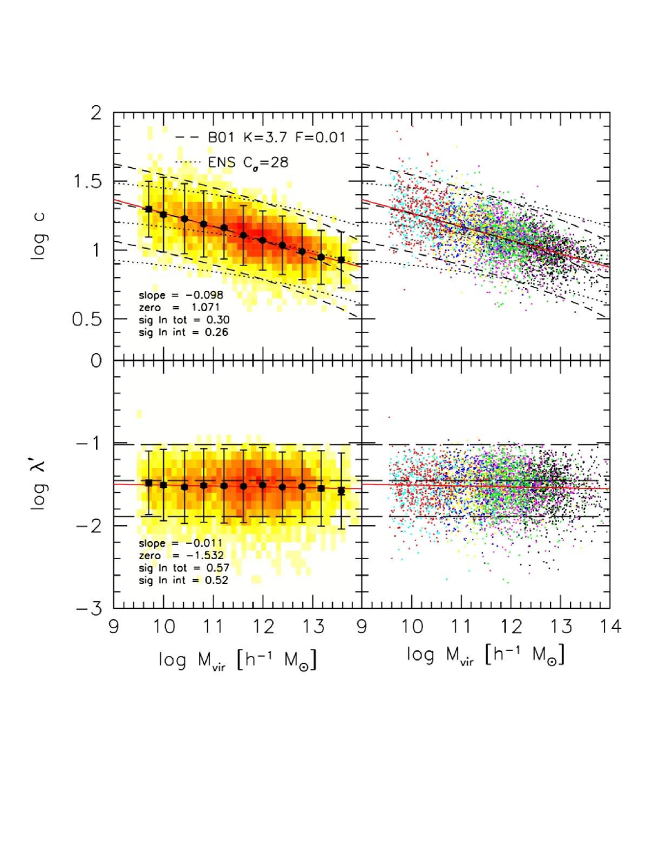
Figure 5: As Fig. 3, but for “relaxed” haloes ($\rho_{\rm rms}<0.4,x_{\rm off}<0.04$). The most notable differences with Fig. 3 are the reduced scatter and shallower slope of the $c-M_{\rm vir}$ relation. See text for further details.

Fig. 5 shows the $c-M_{\rm vir}$ and $\lambda^{\prime}-M_{\rm vir}$ relations for the haloes in the GOOD sub-sample with $N_{\rm vir}>250$. As with the full sample, this $c-M_{\rm vir}$ relation is well fitted with a single power-law given by

$$\log c=1.071[\pm 0.027]-0.098[\pm 0.009](\log M_{\rm vir}-12).$$ (9)

This relation has a slope that is $\sim 10$ percent shallower and a zero point that is $\sim 10$ percent higher than for the full sample (eq. [8]). The total scatter about this mean relation is $\sigma_{\ln c}=0.30\pm 0.03$ and the intrinsic scatter is $\sigma_{\ln c}=0.26\pm 0.03$, about $25$ percent lower than for the full sample. The B01 model again accurately fits the $c-M_{\rm vir}$ relation, but with $K=3.7\pm 0.15$ (for $F=0.01$). For $F=0.001$ the best-fit value for $K$ is $2.9$.

The slope of the $c(M)$ relation for low mass haloes is still consistent with that predicted by the B01 model but steeper than the prediction of the ENS model. Thus, the fact that ENS only compared their model to a small sample of well relaxed haloes can not explain the discrepancy between their results and those of B01. As already eluded to above, the main reason the ENS model was found to be consistent with their own simulations is that the haloes in their simulation only covered a small range in halo masses, over which the difference in slope with respect to the B01 model is difficult to infer.

The slope of the $\lambda^{\prime}-M_{\rm vir}$ relation is again consistent with zero. However, the median is $\sim 15$ percent lower ($\lambda^{\prime}=0.030\pm 0.003$) and the intrinsic scatter is reduced by $\sim 5$ percent ($\sigma_{\ln\lambda^{\prime}}=0.52\pm 0.01$). These differences in $c(M_{\rm vir})$ between the full set of haloes and our GOOD sub-sample are almost identical to those obtained by Wechsler et al. (2002) between all haloes and haloes without a major merger since $z=2$. This reinforces the notion that our GOOD sub-sample consists mostly of haloes which have not experienced a recent major merger.

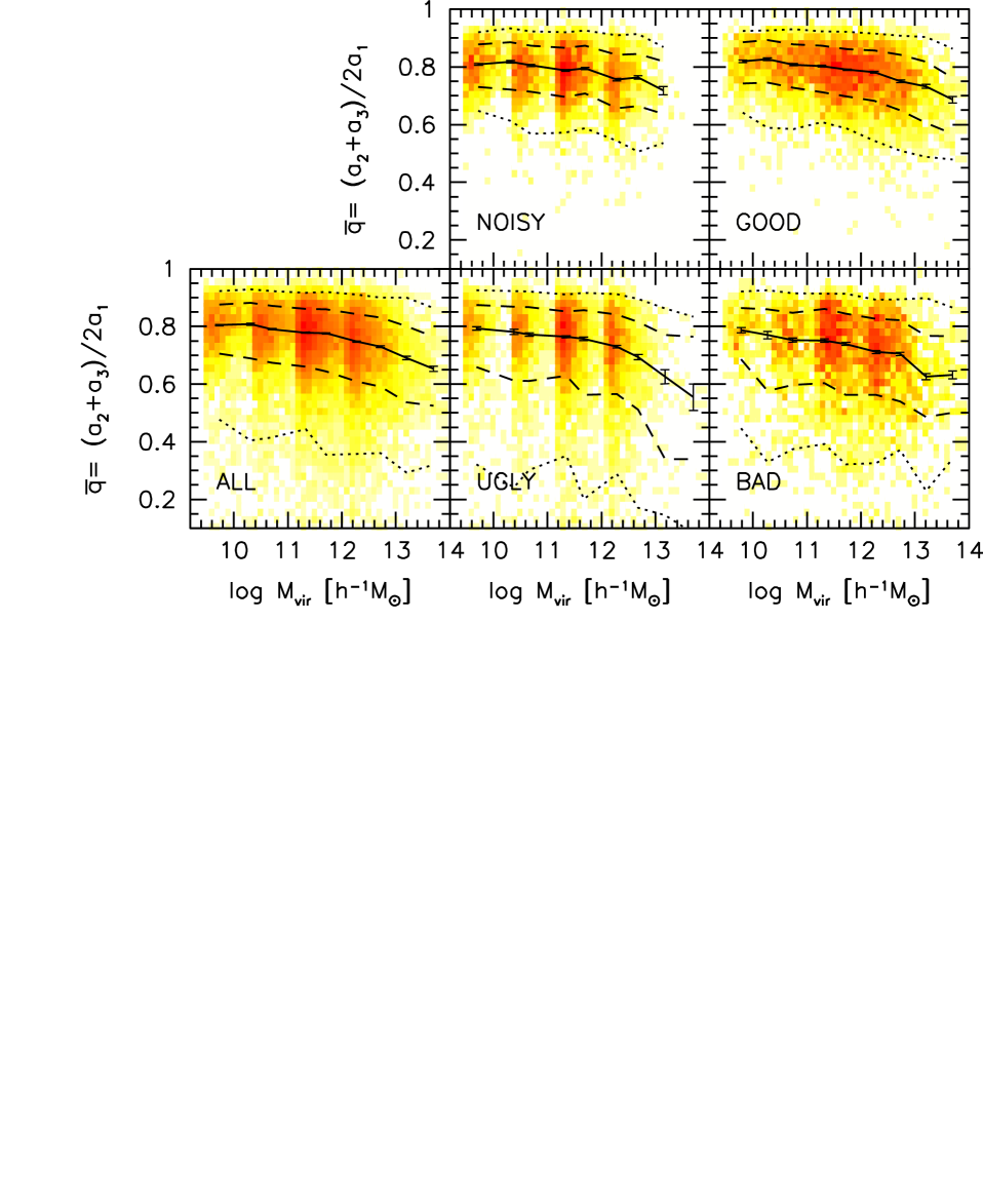
Figure 6: Relation between $\bar{q}$ and $M_{\rm vir}$ for different sub-samples of haloes. The solid lines show the 50th percentile, dashed lines show the 16th and 84th percentiles, and the dotted lines show the 2.5th and 97.5th percentiles. The error bar gives the possion error on the median.

Fig. 6 shows the dependence of the halo shape parameter $\bar{q}$ on halo mass. We find that more massive haloes are on average more flattened (more prolate), in qualitative agreement with previous studies (Jing & Suto 2002; Kasun & Evrard 2005; Bailin & Steinmetz 2005; Allgood et al. 2006). As shown in Allgood et al. (2006), the halo shape is fairly tightly related to the halo assembly time, such that haloes that assemble later are less spherical (and less relaxed). To first order this explains the decrease of $\bar{q}$ with increasing halo mass, as well as the relation between $\bar{q}$ and $x_{\rm off}$ (see Fig. 2). Fig. 6 also shows that haloes with high $x_{\rm off}$ (BAD and UGLY sub-samples) have a lower median $\bar{q}$, as well as a much more pronounced tail to low $\bar{q}$. Note also that there are very few highly prolate haloes ($\bar{q}\mathrel{\hbox to0.0pt{\lower 3.0pt\hbox{$\sim$}\hss}\raise 2.0pt\hbox{$<$}}0.5$) with low $x_{\rm off}$ (NOISY and GOOD sub-samples). A potentially important implication of this is that (LSB) disk galaxies, which are too fragile to survive in unrelaxed haloes, are unlikely to reside in strongly flattened haloes.

4 Correlation between spin and concentration

In their study of the halo angular momentum distributions, Bullock et al. (2001b) noticed that haloes with high $\lambda^{\prime}$ have concentration parameters that are slightly lower than average. Although such a correlation may not be totally unexpected, since both the spin parameter and concentration parameter depend on the mass accretion history (Wechsler et al. 2002; Vitvitska et al. 2002), Bullock et al. argued that the $c$-$\lambda^{\prime}$ anti-correlation is a mere ‘artifact’ from the fact that (i) $c$ and $\lambda$ are uncorrelated (see also NFW), and (ii) $\lambda$ and $\lambda^{\prime}$ are related via $f(c)$ (see Section 2.1.2). However, Bailin et al. (2005) used the $\lambda^{\prime}_{\rm c}$ definition for the spin parameter (which should be equal to $\lambda$) and claimed a significant anti-correlation between halo concentration and spin parameter. As discussed in Bailin et al. (2005), such an anti-correlation may have important implications for the interpretation of the rotation curves of LSB disk galaxies (see discussion in Section 1). Using our large suite of simulations, we therefore re-investigate this issue.

Bailin et al. (2005) focused on haloes with $1\times 10^{11}h^{-1}M_{\odot}<M_{\rm vir}<2\times 10^{12}h^{-1}M_{\odot}$ and $N_{\rm FOF}>1290$. In Fig. 7 we plot the halo concentration as a function of the three different definitions of the spin parameter; $\lambda^{\prime}$, $\lambda^{\prime}_{\rm c}$ and $\lambda$. To facilitate the comparison with Bailin et al. we only select haloes in our simulations with $1\times 10^{11}h^{-1}M_{\odot}<M_{\rm vir}<2\times 10^{12}h^{-1}M_{\odot}$ and $N_{\rm vir}>1000$. All three plots reveal a weak but significant correlation in that the lowest concentration haloes have relatively low spin parameters. Contrary to NFW and Bullock et al. (2001b), but in agreement with Bailin et al. (2005), we therefore argue that $c$ and $\lambda$ are correlated. Note that resolution is not an issue here, since we obtain the same result in each of our different simulations.

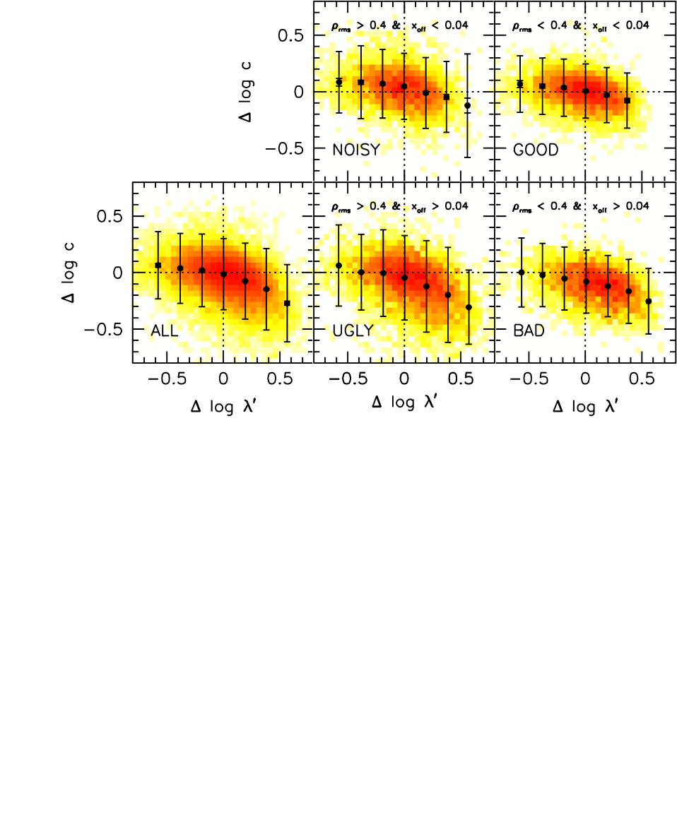
Figure 8: Correlations between the residuals of the $c-M_{\rm vir}$ and $\lambda^{\prime}-M_{\rm vir}$ relations in Fig. 5. The lower left panel shows all haloes, while the remaining panels show the four sub-samples defined according to $\rho_{\rm rms}$ and $x_{\rm off}$ as indicated. The error bars show the 2$\sigma$ scatter in $c$ for each $\Delta\lambda^{\prime}$ bin.

Due to the mass dependence of $c$, a more illustrative way to look for a correlation between halo concentration and spin parameter is to plot the residuals (at constant $M_{\rm vir}$) of the $c-M_{\rm vir}$ and $\lambda^{\prime}-M_{\rm vir}$ relations. This is shown in Fig. 8 for all haloes with $N_{\rm vir}>250$. The lower left panel shows the residuals for the full sample, which reveals a clear trend that haloes with high $\lambda^{\prime}$ have lower than average $c$. We now split the haloes into the four sub-samples defined above, and plot their residuals (with respect to the mean $c(M)$ and mean $\lambda^{\prime}$ for the GOOD sub-sample). This shows that the correlation between $c$ and $\lambda^{\prime}$ is, at least partially, due to the inclusion of haloes with high $x_{\rm off}$ (i.e., haloes that are unrelaxed), independent of whether the halo has a high or low $\rho_{\rm rms}$: the correlation is clearly more pronounced for the UGLY and BAD sub-samples. However, the GOOD and NOISY sub-samples still reveal a small trend that haloes with larger $\lambda^{\prime}$ offsets have a lower $c$ offset. We have repeated this analysis using $\lambda^{\prime}_{\rm c}$ and $\lambda$, and the small correlation between residuals in the GOOD and NOISY sub-samples remains. We therefore conclude that there indeed is a small intrinsic correlation between $c$ and $\lambda^{\prime}$ at a fixed $M_{\rm vir}$. However, when excluding the unrelaxed haloes, the amplitude of this correlation is very weak compared to the scatter in both parameters. In Section 6 below we investigate to what extent this small correlation may effect (LSB) disk galaxies.

5 Environment dependence

We now investigate whether the concentration, spin parameter and shape of dark matter haloes are correlated with the large scale environment in which they are located. This is interesting because disk galaxies, and LSBs in particular, are preferentially found in regions of intermediate to low density (Mo et al. 1994; Rosenbaum & Bomans 2004). If haloes in low density environments have different structural properties than haloes of the same mass in over-dense environments, this would therefore imply that the haloes of (LSB) disk galaxies are not a fair representation of the average halo population.

Using a set of numerical simulations, for different cosmologies, LK99 studied the environment dependence of dark matter haloes. The only halo parameter that was found to be correlated with environment is halo mass (denser environments contain more massive haloes). Halo concentration, spin parameter, shape and assembly redshift were all found to be uncorrelated with halo environment.

However, using exactly the same simulations as LK99, Sheth & Tormen (2004) found clear evidence that halo assembly times correlate with environment based on a marked correlation function analysis. A similar result was obtained by Gao, Springel & White (2005), who used the millennium simulation (Springel et al. 2005) to demonstrate that the low mass haloes that assemble early are more strongly clustered than haloes of the same mass that assemble later. For massive haloes, however, the dependence on the assembly time was found to diminish. This has since been confirmed by a number of studies (Harker et al. 2006; Zhu et al. 2006; Wetzel et al. 2007; Jing, Suto & Mo 2007). In addition, it has been found that the clustering of haloes also depends on other halo properties, such as halo concentration, halo spin parameter, subhalo properties, and the time since the last major merger (Wechsler et al. 2006; Zhu et al. 2006; Wetzel et al. 2007; Gao & White 2007; but see also Percival et al. 2003), which is not too surprising given that all these properties correlate with halo formation time (e.g., Wechsler et al. 2002; van den Bosch, Tormen & Giocoli 2005). All these results seem to overrule the finding by LK99, and seem to suggest that dark matter properties depend rather sensitively on their large scale environment.

Using our large sample of objects, we investigate whether the concentration, spin parameter and shape of haloes are correlated with the large scale environment in which they are located. Rather than using (marked) correlation functions, we follow LK99 and correlate the halo properties with the overdensity, $1+\delta_{r}$, measured in spheres of radius $r$(with $r=1,2,4,8\,{\rm h^{-1}Mpc}$) centered on each halo:

$$1+\delta_{r}=\frac{<\rho(r)>}{\rho_{\rm u}}=\frac{3M(<r)}{4\pi r3}\frac{1}{\rho_{\rm crit}\Omega_{\rm M}}.$$ (10)

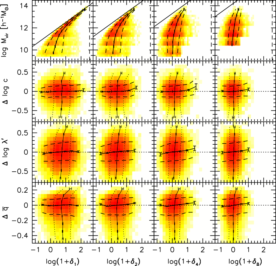
Figure 9: Environment dependence of $M_{\rm vir}$, and of the residuals, at fixed $M_{\rm vir}$ of the $c-M_{\rm vir}$, $\lambda^{\prime}-M_{\rm vir}$ and $\bar{q}-M_{\rm vir}$ relations. Here environment is defined by the matter overdensity within spheres of radii $1,2,4$ and $8\;h^{-1}Mpc$. In the top row the diagonal line shows the minimum overdensity for a halo of a given mass, and the vertical dashed line shows the overdensity at the virial radius. In each panel, the solid curve shows the mean, the error bars indicate the Poisson errors on the mean, and the dashed curves show the $\pm 1\sigma$ scatter in each mass bin. In the second, third and fourth rows the almost vertical lines indicate the average overdensity (plus its error) for haloes in a given residual bin.

The results for all haloes are shown in Fig. 9. The top row shows the relation between virial mass and overdensity. The vertical dashed line shows the overdensity at the virial radius. The solid diagonal line indicates the mass scale $M={4\over 3}\pi(1+\delta_{r})\rho_{\rm crit}\Omega_{\rm M}r^{3}$. Thus all haloes with $R_{\rm vir}$ less than the filter radius should lie below this line, as is the case. Note that we do not include sub-haloes in our analysis, so the only haloes that can have very high densities $\log(1+\delta)\mathrel{\hbox to0.0pt{\lower 3.0pt\hbox{$\sim$}\hss}\raise 2.0pt\hbox{$>$}}2$ must be haloes with virial radii close to the filter radius, as is the case. We see that more massive haloes tend to live in more overdense regions (cf. LK99). As the filter radius is increased the mean overdensity tends towards zero, and the scatter in overdensity is reduced, as expected. Note that we do not compute the overdensity on $8h^{-1}\rm Mpc$ scales in the simulations with the smallest box size.

The second, third and fourth rows of Fig. 9 show the residuals (at fixed $M_{\rm vir}$) of the $c$-$M_{\rm vir}$, $\lambda^{\prime}$-$M_{\rm vir}$ and $\bar{q}$-$M_{\rm vir}$ relations, respectively, all as function of overdensity. The roughly horizontal lines with errorbars indicate the mean residual (plus its errors) as function of overdensity, while the dashed lines outline the $\pm 1\sigma$ scatter. Note that, within the errors on the mean, there is no significant indication that the residuals are larger or smaller in regions that are over- or under-dense. In other words, these results are in excellent agreement with those of LK99 and seem to suggest that halo properties are independent of their large scale environment. Note that our results cover a much wider dynamic range in halo mass, and are based on higher-resolution simulations than in the case of LK99. How can this be reconciled with the findings based on the correlation function analyses described above? Some insight is provided by the roughly vertical lines with errorbars (in the second, third and fourth rows of Fig. 9), which indicate the average overdensity (plus its error) for haloes in a given residual bin. The corresponding dotted lines outline the $\pm 1\sigma$ scatter. These show that haloes with the largest concentration, largest spin parameter, and/or that are most spherical (all with respect to the average for their mass) are located in slightly denser environments. Since the correlation function reflects ensemble averages, this seems consistent with the findings that more concentrated haloes and/or those with a larger spin parameter are more strongly clustered. We emphasize, though, that the trends seen in Fig. 9 are (i) weaker when environment is measured over a larger volume, (ii) only reveal an environment dependence at the extremes of the residual distributions, and (iii) largely vanish when we only focus on haloes in our GOOD sub-sample (not shown).

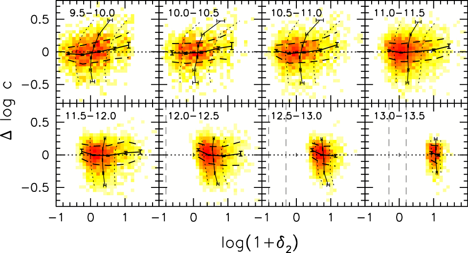
Figure 10: Environment dependence of the residuals, at fixed $M_{\rm vir}$, of the $c-M_{\rm vir}$ relation. Different panels correspond to different halo mass bins, as indicated (numbers indicate $\log[M_{\rm vir}/h^{-1}M_{\odot}]$). The solid curve shows the mean, the error bars show the Poisson error on the mean, and the dashed curves show the $\pm 1\sigma$ scatter. The dashed lines show the overdensity corresponding to a single halo in a sphere of radius $2{\rm h^{-1}Mpc}$ with a mass equal to the lower and upper mass limits of each panel. The almost vertical lines have the same meaning of Fig. 9 indicating the average overdensity (plus its error) for haloes in a given residual bin.

As emphasized in Harker et al. (2006), in order to reveal the correlation between environment and assembly time, it is important to only consider haloes in a relatively small mass range. Therefore, in Fig. 10 we plot the residuals of the $c-M_{\rm vir}$ relation versus overdensity in $2{\rm h^{-1}Mpc}$ spheres for haloes in mass bins with a width of 0.5 dex. The various lines and errorbars have the same meaning as in Fig. 9. For haloes with $M_{\rm vir}\mathrel{\hbox to0.0pt{\lower 3.0pt\hbox{$\sim$}\hss}\raise 2.0pt\hbox{$<$}}10^{12}h^{-1}M_{\odot}$ there is a weak, mildly significant indication that haloes in denser environments have slightly higher concentrations (reflected by close-to-horizontal lines). More pronounced, however, is the trend that more concentrated haloes live on average in denser environments (reflected by close-to-vertical lines). This is consistent with the fact that more concentrated, low mass haloes are more strongly clustered (cf. Wechsler et al. 2006). It is clear from Fig. 10 that the environment dependence is weaker for more massive haloes; in fact for haloes in the mass range $12\mathrel{\hbox to0.0pt{\lower 3.0pt\hbox{$\sim$}\hss}\raise 2.0pt\hbox{$<$}}\log[M/(h^{-1}M_{\odot})]\mathrel{\hbox to0.0pt{\lower 3.0pt\hbox{$\sim$}\hss}\raise 2.0pt\hbox{$<$}}13.5$ no significant environment dependence is seen (this explains why the signal is weaker in Fig. 9 where we add all the masses together). Again this is in good agreement with the clustering results of Wechsler et al. (2006) and Gao & White (2007), who found that the dependence on halo concentration vanishes for haloes with masses close to the typical collapsing mass, $M^{*}$: for the cosmology assumed in our simulations $M^{*}=6.7\times 10^{12}h^{-1}M_{\odot}$. Thus, our results are in good agreement with the various claims based on correlation function analyses. They also illustrate, though, that the trends are weak compared to the scatter, which explains why LK99 did not notice any environment dependence. Only when one carefully estimates the average environment as function of halo property, which is what a correlation function measures, does the environment dependence reveal itself.

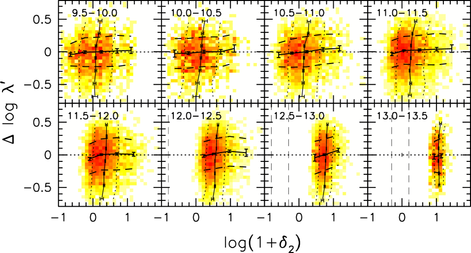
Figure 11: Same as Fig. 10, except that here we show the residuals of the $\lambda^{\prime}-M_{\rm vir}$ relation.

Figure 11 shows the residuals, at fixed $M_{\rm vir}$, of the $\lambda^{\prime}-M_{\rm vir}$ relation as function of $\log(1+\delta_{2})$ for the same mass bins as in Fig. 10. Unlike the concentration, the spin parameter reveals no significant environment dependence, in any mass bin. This is inconsistent with Gao & White (2007) who found that higher spin haloes are more strongly clustered than low spin haloes of the same mass. It is unclear why our analysis of the environmental densities does not recover this trend, while it does reproduce the trend for the halo concentrations.

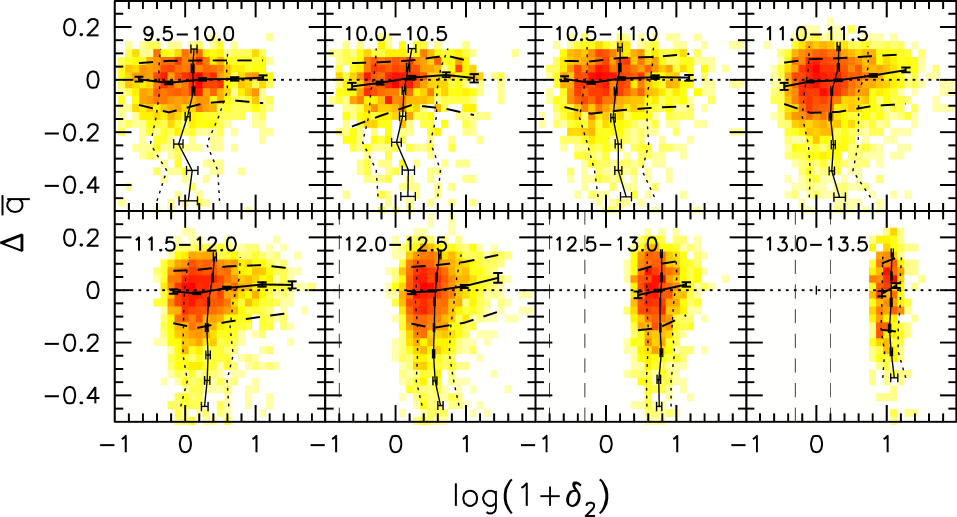
Figure 12: Same as Fig. 10, except that here we show the residuals of the $\bar{q}-M_{\rm vir}$ relation.

Finally, Fig. 12 shows the same as Figs 10 and 11 but for the shape parameter $\bar{q}$. As for the spin parameter, there is no indication for any significant environment depencence. This seems at odds with Fig. 9 (fourth row), which shows that the most spherical haloes (those with large positive $\Delta\bar{q}$) live in denser environments. This apparent discrepancy simply reflects number statistics: only the haloes in the bin with $\Delta\bar{q}>0.2$ seem to reside in regions that are denser than average. When split in mass bins, however, there are too few haloes with $\Delta\bar{q}>0.2$ to reveal the signal.

6 The Host Haloes of LSB Disk Galaxies

We now investigate whether LSB disk galaxies are expected to reside in dark matter haloes that form a biased sub-set in terms of their concentration parameters. In the MMW model the central surface density of an exponential disk, $\Sigma_{0,\rm d}$, is determined by $\lambda$, $c$, $M_{\rm vir}$, and the galaxy mass fraction $m_{\rm gal}$ (defined as the ratio between disk mass and halo mass). A lower $\Sigma_{0,\rm d}$ will result from

• a higher $\lambda$ at fixed $c$, $M_{\rm vir}$, and $m_{\rm gal}$;

• a lower $M_{\rm vir}$ at fixed $c$, $\lambda$, and $m_{\rm gal}$;

• a lower $c$ at fixed $\lambda$, $M_{\rm vir}$, and $m_{\rm gal}$;

• a lower $m_{\rm gal}$ at fixed $c$, $\lambda$, and $M_{\rm vir}$.

To complicate matters, lower mass haloes have higher concentrations, $\lambda$ and $c$ are weakly anti-correlated (see Section 4), and $m_{\rm gal}$ is expected to increase with $M_{\rm vir}$ due to various astrophysical feedback processes.

To investigate the impact of all these relations on the surface brightness of disk galaxies, we construct MMW type models as described in Dutton et al. (2007). These models consist of an exponential disk, a Hernquist bulge and a NFW halo. The halo parameters are $M_{\rm vir}$, $c$ and $\lambda^{\prime}_{\rm c}$ ($\equiv\lambda$), which we take directly from the haloes of our GOOD sub-sample. An additional parameter is the galaxy mass fraction $m_{\rm gal}$, which we fix to $m_{\rm gal}=0.04$ for simplicity. The bulge formation recipe is based on disk instability, and therefore only effects the highest surface brightness disks; the details of this bulge formation recipe are not important for this work. We assume that the halo is unaffected by the formation of the disk, i.e. we do not consider adiabatic contraction. As highlighted in Dutton et al. (2007), models with adiabatic contraction are unable to simultaneously match the zero-point of the Tully-Fisher relation and the galaxy luminosity function.

The MMW formalism gives the galaxy mass, $M_{\rm gal}$, baryonic disk scale length, $R_{\rm d}$, and central surface density of the baryonic disk, $\Sigma_{0,\rm d}$. As described in Dutton et al. (2007), we split the disk into a stellar and a gaseous component assuming that all disk material with a surface density $\Sigma(R)>\Sigma_{\rm crit}(R)$ has been turned into stars. Here $\Sigma_{\rm crit}$ is the star formation threshold density, modeled as the critical surface density given by Toomre’s stability criterion (Toomre 1964; Kennicutt 1989).The resulting stellar surface density profile is fitted with an exponential profile to obtain the scale length of the stellar disk, $R_{*}$, and the central surface density of the stellar disk, $\Sigma_{0,*}$. Note that in general $R_{*}<R_{\rm d}$.

In order to facilitate a comparison with observations we convert $\Sigma_{0,\rm*}$ into $\mu_{0,\rm B}$, the central surface brightness of the stellar disk in the B-band, using the B-band stellar mass-to-light ratio, $\Upsilon_{\rm B}$. Using data from Dutton et al. (2007) and relations between mass-to-light ratios and color from Bell et al. (2003) we obtain

$$\log\Upsilon_{B}=0.06+0.25\log\left({M_{*}\over 10^{10}M_{\odot}}\right)$$ (11)

where we have adopted a Kennicutt IMF and a Hubble constant $h=0.7$. In principle this relation has a scatter of $\simeq 0.1$ dex, which we ignore for simplicity.

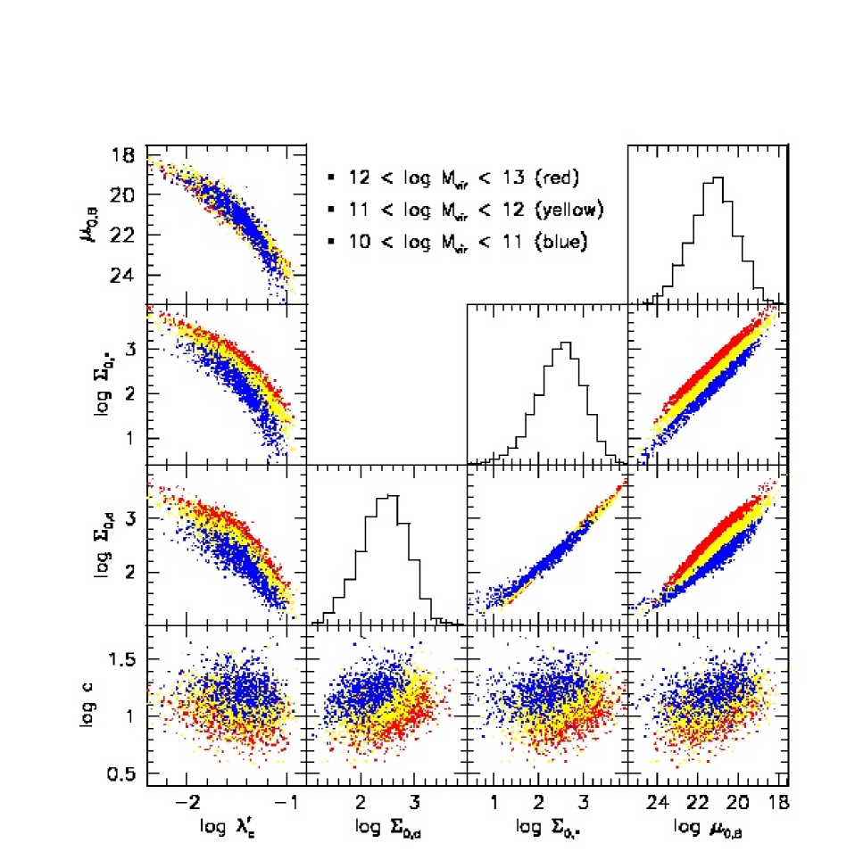
Figure 13: Correlations between the halo variables $\lambda^{\prime}_{\rm c}$ and $c$ with the galaxy properties $\Sigma_{0}$ (baryonic disk central surface density, units of $M_{\odot}\,\rm pc^{-2}$), $\Sigma_{0,*}$ (stellar disk central surface density, units $M_{\odot}\,\rm pc^{-2}$), and $\mu_{0,B}$ (stellar disk central surface brightness in the B-band, units $\rm magn.\,arcsec^{-2}$), for haloes with $N_{\rm vir}>250$, $\rho_{\rm rms}<0.4$, and $x_{\rm off}<0.04$ (i.e. relaxed haloes). The points are color coded according to $M_{\rm vir}$ (units $h^{-1}\,\rm M_{\odot}$) as indicated.

Fig. 13 shows correlations between $c$, $\lambda^{\prime}_{\rm c}$, $\Sigma_{0,\rm d}$ (central surface density of baryonic disk), $\Sigma_{0,*}$ (central surface density of stellar disk), and $\mu_{0,B}$ (central surface brightness in the B-band) and histograms of $\Sigma_{0,\rm d}$, $\Sigma_{0,*}$ and $\mu_{0,B}$ for GOOD haloes in the mass range $10^{10}h^{-1}M_{\odot}<M_{\rm vir}<10^{13}h^{-1}M_{\odot}$. The distributions of $\Sigma_{0,\rm d}$, $\Sigma_{0,*}$ and $\mu_{0,\rm B}$ are approximately log-normal, reflecting the log-normal distribution of $\lambda^{\prime}_{\rm c}$. The distribution of $\mu_{0,\rm B}$ has a peak value in agreement with the Freeman value of 21.65 magn. arcsec^-2.

As expected, there is a strong correlation between $\Sigma_{0,\rm d}$ and $\lambda^{\prime}_{\rm c}$, in that haloes with larger spin parameters host lower surface density disks. The flattening of this relation at low $\lambda^{\prime}_{\rm c}$ owes to our bulge formation recipe. At fixed $\lambda^{\prime}_{\rm c}$, more massive haloes have higher $\Sigma_{0,\rm d}$, despite their (on average) smaller concentrations. The scatter in $c$ at a fixed $M_{\rm vir}$ results in some overlap between the three mass samples, but the three mass ranges are clearly visible. Thus, the dependence of surface density on halo mass is at least as important as the dependence on halo concentration. The same trends are seen in the relation between surface density of the stellar disk and spin parameter. However the mass separation is no longer present in the relation between surface brightness and spin parameter. This is because, at a given $\Sigma_{0,*}$, more massive haloes have higher stellar mass-to-light ratios, and hence lower surface brightness.

The lower left panel of Fig. 13 plots the halo concentration versus the halo spin parameter. Although these parameters seem uncorrelated, there is a weak anti-correlation between $c$ and $\lambda^{\prime}_{\rm c}$, as discussed in Section 4. The fact that this correlation is not as pronounced as in Fig. 7, is due to the fact that here we only consider the GOOD sub-sample. The other three panels in the lower row show the correlation between halo concentration and disk surface density (or brightness). For haloes of a given mass, there is a clear correlation in that more concentrated haloes host higher surface density (brightness) disks. This correlation has two origins: centrifugal equilibrium and the (weak) correlation between $\lambda^{\prime}_{\rm c}$ and $c$. In what follows we investigate the relative importance of both of these causes.

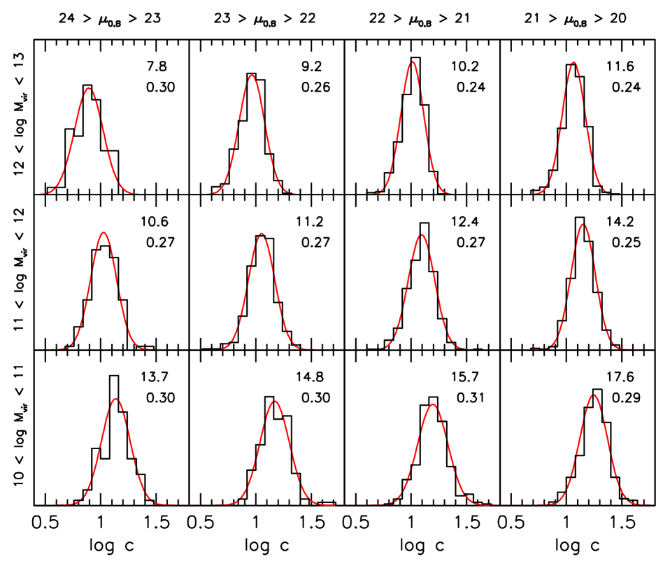
Figure 14: Histograms of concentration parameter for different viral masses (units of $h^{-1}\,\rm M_{\odot}$) and B-band central surface brightness (units of $\rm magn.\,arcsec^{-2}$) for the model galaxies in Fig. 13. The three mass ranges (from top to bottom) correspond to massive, intermediate and dwarf galaxies, while the four surface brightness ranges (from left to right) correspond to low, intermediate, high and very high surface brightness. For each subset of haloes the red line shows a gaussian distribution with a mean $c$ and standard deviation $\sigma_{\ln c}$ as given in the top right corner of each panel. Note that the dependence on mass is much stronger than the dependence on surface brightness.

Fig. 14 shows the distribution of $c$ for different ranges of $M_{\rm vir}$ and $\mu_{0,\rm B}$. The three mass ranges roughly correspond to massive galaxies ($150\mathrel{\hbox to0.0pt{\lower 3.0pt\hbox{$\sim$}\hss}\raise 2.0pt\hbox{$<$}}V_{\rm vir}\mathrel{\hbox to0.0pt{\lower 3.0pt\hbox{$\sim$}\hss}\raise 2.0pt\hbox{$<$}}300\,\rm km\,s^{-1}$), intermediate mass galaxies ($70\mathrel{\hbox to0.0pt{\lower 3.0pt\hbox{$\sim$}\hss}\raise 2.0pt\hbox{$<$}}V_{\rm vir}\mathrel{\hbox to0.0pt{\lower 3.0pt\hbox{$\sim$}\hss}\raise 2.0pt\hbox{$<$}}150\,\rm km\,s^{-1}$), and dwarf galaxies ($30\mathrel{\hbox to0.0pt{\lower 3.0pt\hbox{$\sim$}\hss}\raise 2.0pt\hbox{$<$}}V_{\rm vir}\mathrel{\hbox to0.0pt{\lower 3.0pt\hbox{$\sim$}\hss}\raise 2.0pt\hbox{$<$}}70\,\rm km\,s^{-1}$). At a fixed surface brightness, less massive haloes have higher $c$ as expected. At a fixed halo mass, there is a clear trend that lower surface brightness disks reside in less concentrated haloes. If we define LSB galaxies as those with a central surface brightness $24\mathrel{\hbox to0.0pt{\lower 3.0pt\hbox{$\sim$}\hss}\raise 2.0pt\hbox{$>$}}\mu_{0,\rm B}\mathrel{\hbox to0.0pt{\lower 3.0pt\hbox{$\sim$}\hss}\raise 2.0pt\hbox{$>$}}23\,{\rm magn.}{\rm arcsec}^{-2}$, we find that they live in a sub-set of haloes whose average concentration (at fixed halo mass) is $\sim 15$ percent lower than the overall average for that halo mass. We therefore conclude halo concentrations inferred from LSB rotation curves should not be compared to $\langle c\rangle_{M}$, but rather to $f\langle c\rangle_{M}$, with $f\simeq 0.85$ a bias correction factor. A similar conclusion was obtained by Bailin et al. (2005), except that they found a bias correction factor of $f\simeq 0.70$. As discussed in Section 4 this owes to the fact that they did not remove unrelaxed haloes from their sample. Since we consider it unlikely that LSB galaxies reside in unrelaxed haloes, we belief our bias correction factor to be more realistic.

Finally, in order to investigate the origin of this bias, we have run a control sample with the same distributions of $M_{\rm vir}$, $c$ and $\lambda^{\prime}_{\rm c}$ as the simulation data, but with no correlation between $c$ and $\lambda^{\prime}_{\rm c}$. This reduces the correction factor to $f\simeq 0.95$, and therefore shows that the main contribution to $f$ owes to the (very weak) anti-correlation between halo concentration and halo spin parameter. The remaining contribution simply reflects that centrifugally supported disks in less concentrated haloes will be less concentrated themselves.

7 Summary

In this paper we have used a set of cosmological N-body simulations to study the scaling relations, at redshift zero, between the concentration parameter, $c$, spin parameter, $\lambda^{\prime}$, shape parameter, $\bar{q}$, and mass, $M_{\rm vir}$, of a large sample of dark matter haloes. Due to the combined set of simulations, we were able to extend previous studies to a mass range at least an order of magnitude smaller, covering the full range of masses in which galaxies are expected to form: $3\times 10^{9}h^{-1}\,\rm M_{\odot}\mathrel{\hbox to0.0pt{\lower 3.0pt\hbox{$\sim$}\hss}\raise 2.0pt\hbox{$<$}}M_{\rm vir}\mathrel{\hbox to0.0pt{\lower 3.0pt\hbox{$\sim$}\hss}\raise 2.0pt\hbox{$<$}}3\times 10^{13}h^{-1}\,\rm M_{\odot}$.

For this mass range we find $c\propto M_{\rm vir}^{-0.11}$, which is in agreement with the model of Bullock et al. (2001a), but in disagreement with the model of Eke, Navarro & Steinmetz (2001) which predicts a significantly shallower slope. The single free parameter of the ENS model only controls the normalization of the $c-M_{\rm vir}$ relation, so that their model cannot be tuned to fit the data. The ENS model has also been shown to be unable to match the slope of the $c-M_{\rm vir}$ relation for low mass haloes at $z=3$ (Colín et al. 2004). For the Bullock et al. (2001a) model our data is well fitted with a model with $F=0.01$ and $K=3.4\pm 0.1$ (where the error reflects our estimate of cosmic variance). Note that this normalization is 15 percent lower than the $K=4.0$ originally proposed by Bullock et al. (2001a), but it is in good agreement with Zhao et al. (2003) and Kuhlen et al. (2005), who found a best-fit normalization of $K=3.5$. This discrepancy is at least partially due to an inconsistency with the use of transfer functions in the work of Bullock et al. If they use the same transfer functions to set up the initial conditions of their simulations and to compute the model predictions, they obtain $K=3.75$. This is however significantly higher than can be accounted for by our estimate of cosmic variance. We find an intrinsic scatter in $c$ and $\lambda^{\prime}$ at fixed $M_{\rm vir}$ of $\sigma_{\ln c}=0.33\pm 0.03$ and $\sigma_{\ln\lambda}=0.55\pm 0.01$, and a median spin parameter of $\lambda^{\prime}=0.034\pm 0.001$, all in good agreement with Bullock et al. (2001a,b).

In an attempt to distinguish between relaxed and unrelaxed haloes we introduce a new and simple parameter: $x_{\rm off}$ which is defined as the distance between the most bound particle and the center of mass, in units of the virial radius. The distribution of $x_{\rm off}$ is approximately log-normal with a median $\overline{x}_{\rm off}\simeq 0.04$. The full set of haloes shows strong correlations between $x_{\rm off}$ and the residuals of the $c-M_{\rm vir}$ and $\lambda^{\prime}-M_{\rm vir}$ relations, such that haloes with larger $x_{\rm off}$ have a larger than average $\lambda^{\prime}$ and a lower than average $c$. Removing haloes with large $x_{\rm off}$ therefore results in a higher mean concentration, a lower mean spin parameter, and in less scatter in both the $c-M_{\rm vir}$ and $\lambda^{\prime}-M_{\rm vir}$ relations. The median spin parameter of ‘relaxed’ (GOOD) haloes is $\lambda^{\prime}=0.030\pm 0.003$ with an intrinsic scatter of $\sigma_{\ln\lambda^{\prime}}=0.52\pm 0.01$. The average $c(M_{\rm vir})$ of ‘relaxed’ haloes is again in good agreement with the model of B01, but with $F=0.01$ and $K=3.7$, and with a reduced intrinsic scatter of $\sigma_{\ln c}=0.26\pm 0.03$.

A better fit to the $c-M_{\rm vir}$ relation for high mass haloes ($M_{\rm vir}\mathrel{\hbox to0.0pt{\lower 3.0pt\hbox{$\sim$}\hss}\raise 2.0pt\hbox{$>$}}10^{13}h^{-1}\,\rm M_{\odot}$) can be obtained with $F=0.001$ and $K=2.6$ (for all haloes), and $K=2.9$ (for GOOD haloes). This is, however, at the expense of under predicting the concentrations for the low mass haloes ($M_{\rm vir}\mathrel{\hbox to0.0pt{\lower 3.0pt\hbox{$\sim$}\hss}\raise 2.0pt\hbox{$<$}}10^{11}h^{-1}\,\rm M_{\odot}$).

We also find a strong correlation between the mean axis ratio of the haloes, $\bar{q}$, and $x_{\rm off}$, such that more prolate haloes (i.e., those with lower $\bar{q}$) have higher $x_{\rm off}$, on average. This suggests that the majority of haloes with small axis ratios are unrelaxed, and thus that fragile LSB galaxies are unlikely to reside in haloes that are strongly aspherical. This makes it less likely that the discrepancy between observed and predicted rotation curves is due to the fact that disks are strongly elliptical, as suggested by Hayashi et al. (2004).

We have also investigated the environment dependence of the residuals in $c$ and $\lambda^{\prime}$. This is interesting because disk galaxies, and LSBs in particular, are preferentially found in regions of intermediate to low density (Mo et al. 1994; Rosenbaum & Bomans 2004). Defining ‘environment’ by the matter overdensity within spheres of radii $1,2,4$ and $8h^{-1}$Mpc, we find at the low mass end ($M<M^{*}$) that more concentrated haloes live in denser environments than their less concentrated counterparts of the same mass. This is consistent with the studies of Wechsler et al. (2006) and Gao & White (2007) who found a similar trend using correlation functions. However, as we have shown, this trend is weak compared to the scatter, which explains why Lemson & Kauffmann (1999) did not notice any environment dependence in their simulation. Contrary to the halo concentrations, the halo spin parameters reveal no environment dependence at fixed mass. This is at odds with the results of Gao & White (2007) who found that haloes with a large spin parameter are more strongly clustered than low spin haloes of the same mass. Finally we find a weak trend that the most spherical haloes reside in slightly denser environments.

Finally, using a simple model for disk galaxy formation, we investigated the properties of the (expected) host haloes of LSB disk galaxies (i.e., those with a central surface brightness $24\mathrel{\hbox to0.0pt{\lower 3.0pt\hbox{$\sim$}\hss}\raise 2.0pt\hbox{$>$}}\mu_{0,\rm B}\mathrel{\hbox to0.0pt{\lower 3.0pt\hbox{$\sim$}\hss}\raise 2.0pt\hbox{$>$}}23\,{\rm magn.}{\rm arcsec}^{-2}$). In addition to having higher than average spin parameters, in agreement with numerous other studies (e.g., Dalcanton et al. 1997; Jimenez et al. 1998), we also find that the host haloes of LSB galaxies have concentrations that are biased low by about 15 percent. This correlation between halo concentration and disk surface brightness (or density) owes largely to a (weak) anti-correlation between $\lambda^{\prime}$ and $c$, and to the fact that centrifugal equilibrium commands that less concentrated haloes host less concentrated disks. The amplitude of this correlation is significantly smaller than what has been advocated by Bailin et al. (2005), but this owes to the fact that these authors did not remove unrelaxed haloes, which are unlikely to host fragile LSB galaxies, from their analysis.

All these results have important implications for the interpretation of the halo concentrations inferred from LSB rotation curves. Numerous studies in the past have argued that these are too low compared to the predictions for a $\Lambda$CDM cosmology (e.g., Alam et al. 2002; McGaugh et al. 2003; de Blok et al. 2003). However, there are several reasons why we now believe that the model predictions where too high. First of all, virtually all previous predictions were made for a flat $\Lambda$CDM cosmology with $\Omega_{m}=0.3$ and $\sigma_{8}=0.9$ (or $\sigma_{8}=1.0$). However, if one adopts the cosmology favored by the three year data release of the WMAP mission (Spergel et al. 2006), one predicts concentrations that are about 25 percent lower (Macciò et al. , in preparation). Compared to a $\Lambda$CDM model with $\Omega_{m}=0.3$ and $\sigma_{8}=1.0$ the concentrations are 35 percent lower. Secondly, the B01 model (with $F=0.01$ and $K=4.0$) overpredicts the halo concentrations by $\sim 15$ percent. If we take into account that LSBs only reside in relaxed haloes, this is lowered to a $\sim 8$ percent effect. And finally, one needs to correct for the fact that LSB galaxies reside in a biased sub-set of haloes, which is another 15 percent effect. Combining all these effects, it is clear that the halo concentrations predicted were almost a factor two too large. This brings models and data into much better agreement.

Figure 7: Correlations between $c$ and $\lambda^{\prime}$, $\lambda^{\prime}_{\rm c}$ and $\lambda$ for haloes with $1\times 10^{11}<M_{\rm vir}<2\times 10^{12}\;h^{-1}M_{\odot}$ and $N_{\rm vir}>1000$.

References

- Alam et al. (2002) Alam, S. M. K., Bullock, J. S., & Weinberg, D. H. 2002, ApJ, 572, 34
- Allgood et al. (2006) Allgood, B., Flores, R. A., Primack, J. R., Kravtsov, A. V., Wechsler, R. H., Faltenbacher, A., & Bullock, J. S. 2006, MNRAS, 367, 1781
- Avila-Reese et al. (2005) Avila-Reese, V., Colín, P., Gottlöber, S., Firmani, C., & Maulbetsch, C. 2005, ApJ, 634, 51
- Bailin & Steinmetz (2005) Bailin, J., & Steinmetz, M. 2005, ApJ, 627, 647
- Bailin et al. (2005) Bailin, J., Power, C., Gibson, B. K., & Steinmetz, M. 2005, preprint(astro-ph/0502231)
- Bell et al. (2003) Bell, E. F., McIntosh, D. H., Katz, N., & Weinberg, M. D. 2003, ApJS, 149, 289
- Bertschinger (2001) Bertschinger, E. 2001, ApJS, 137, 1
- Blumenthal et al. (1986) Blumenthal, G. R., Faber, S. M., Flores, R., & Primack, J. R., 1986, ApJ, 301, 27
- Bullock et al. (2001a) Bullock, J. S., Kolatt, T. S., Sigad, Y., Somerville, R. S., Kravtsov, A. V., Klypin, A. A., Primack, J. R., & Dekel, A. 2001a, MNRAS, 321, 559 (B01)
- Bullock et al. (2001b) Bullock, J. S., Dekel, A., Kolatt, T. S., Kravtsov, A. V., Klypin, A. A., Porciani, C., & Primack, J. R. 2001b, ApJ, 555, 240
- Colín et al. (2004) Colín, P., Klypin, A., Valenzuela, O., & Gottlöber, S. 2004, ApJ, 612, 50
- Dalcanton et al. (1997) Dalcanton, J .J., Spergel, D. N., & Summers, F. J. 1997, ApJ, 482, 659
- de Blok et al. (2003) de Blok, W. J. G., Bosma, A., McGaugh, S. S. 2003, MNRAS, 340, 657
- D’Onghia & Burkert (2004) D’Onghia, E., & Burkert, A. 2004, ApJL, 612, L13
- Dutton et al. (2005) Dutton, A. A., Courteau, S., de Jong, R., & Carignan, C. 2005, ApJ, 619, 218
- Dutton et al. (2007) Dutton, A. A., van den Bosch, F. C., Dekel, A., & Courteau, S. 2007, ApJ, 654, 27
- Eke et al. (2001) Eke, V. R., Navarro, J. F., & Steinmetz, M. 2001, ApJ, 554, 114
- Gao et al. (2005) Gao, L., Springel, V., & White, S. D. M., 2005, MNRAS, 363, 66
- Gao & White (2006) Gao, L., & White, S. D. M., 2006, preprint (astro-ph/0611921)
- Gnedin et al. (2006) Gnedin, O. Y., Weinberg, D. H., Pizagno, J., Prada, F., & Rix, H. W., 2006, preprint (astro-ph/0607394)
- Harker et al. (2006) Harker, G., Cole, S., Helly, J., Frenk, C., & Jenkins, A. 2006, MNRAS, 367, 1039
- Hayashi etal. (2004) Hayashi, E., et al. 2004, preprint (astro-ph/0408132)
- Holley-Bockelmann et al. (2005) Holley-Bockelmann, K., Weinberg, M., & Katz, N. 2005, MNRAS, 363, 991
- Jimenez et al. (1998) Jimenez, R., Padoan, P., Matteucci, F., & Heavens, A. F. 1998, MNRAS, 299, 123
- Jing (2000) Jing, Y. P. 2000, ApJ, 535, 30
- Jing & Suto (2002) Jing, Y. P., & Suto, Y. 2002, ApJ, 574, 538
- Jing et al. (2006) Jing, Y. P., Suto, Y., & Mo, H. J., 2006, preprint (astro-ph/0610099)
- Kasun & Evrard (2005) Kasun, S. F., & Evrard, A. E. 2005, ApJ, 629, 781
- Kennicutt (1989) Kennicutt, R. C. Jr., 1989, ApJ, 344, 685
- Kuhlen et al. (2005) Kuhlen, M., Strigari, L. E., Zentner, A. R., Bullock, J. S., & Primack, J. R. 2005, MNRAS, 357, 387
- Lemson & Kauffmann (1999) Lemson, G., & Kauffmann, G. 1999, MNRAS, 302, 111
- Ma & Bertschinger (1995) Ma, C. P., & Bertschinger, E. 1995, ApJ, 455, 7
- Macciò et al. (2003) Macciò, A. V., Murante, G., & Bonometto, S. A. 2003, ApJ, 588, 35
- Maller et al. (2002) Maller, A. H., Dekel, A., & Somerville, R.S., 2002, MNRAS, 329, 423
- Mainini et al. (2003) Mainini, R., Macciò, A. V., Bonometto, S. A., & Klypin, A. 2003, ApJ, 599, 24
- McGaugh et al. (2003) McGaugh, S. S., Barker, M. K., de Blok, W. J. G. 2003, ApJ, 584, 566
- Mo et al. (1994) Mo, H. J., McGaugh, S. S., & Bothun, G. D. 1994, MNRAS, 267, 129
- Mo et al. (1998) Mo, H. J., Mao, S., & White, S. D. M. 1998, MNRAS, 295, 319 (MMW)
- Mo & Mao (2004) Mo, H. J., & Mao, S. 2004, MNRAS, 353, 829
- Navarro et al. (1997) Navarro, J. F., Frenk, C. S., & White, S. D. M. 1997, ApJ, 490, 493 (NFW)
- Peebles (1969) Peebles 1969, ApJ, 155, 393
- Percival et al. (2003) Percival, W. J., Scott, D., Peacock, J. A., & Dunlop, J. S., 2003, MNRAS, 338, 31
- Rhee et al. (2004) Rhee, G., Valenzuela, O., Klypin, A., Holtzman, J., & Moorthy, B. 2004, ApJ, 617, 1059
- Rosenbaum & Bomans (2004) Rosenbaum, S. D., & Bomans, D. J. 2004, A&A, 422, L5
- Shaw et al. (2006) Shaw, L. D., Weller, J., Ostriker, J. P., & Bode, P. 2006, ApJ, 646, 815
- Sheth & Tormen (2002) Sheth, R. K., & Tormen, G. 2002, MNRAS, 329, 61
- Sheth & Tormen (2004) Sheth, R. K., & Tormen, G. 2004, MNRAS, 350, 1385
- Spergel et al. (2003) Spergel, D. N., et al. 2003, ApJS, 148, 175
- Spergel et al. (2006) Spergel, D. N., et al. 2006, preprint (astro-ph/0603449)
- Springel et al. (2005) Springel, V., et al. 2005, Nature, 435, 629
- Stadel (2001) Stadel, J. G. 2001, Ph.D. Thesis, University of Washington
- Spekkens et al. (2005) Spekkens, K., Giovanelli, R., & Haynes, M. P. 2005, AJ, 129, 2119
- Swaters et al. (2003) Swaters, R. A., Madore, B. F., van den Bosch, F. C., & Balcells, M. 2003, ApJ, 583, 732
- Tonini (2006) Tonini, T., Lapi, A., & Salucci, P. 2006, ApJ, 649, 591
- Toomre (1964) Toomre, A., 1964, ApJ, 139, 1217
- Tully & Fisher (1977) Tully, R. B., & Fisher, J. R. 1977, A&A, 54, 661
- van den Bosch (2000) van den Bosch, F. C. 2000, ApJ, 530, 177
- van den Bosch et al. (2002) van den Bosch, F. C., Abel, T., Croft, R.A.C., Hernquist, L., & White, S.D.M., 2002, ApJ, 576, 21
- van den Bosch et al. (2003) van den Bosch, F. C., Mo, H. J., & Yang, X. 2003, MNRAS, 345, 923
- van den Bosch et al. (2005) van den Bosch, F. C., Tormen, G., & Giocoli, C., 2005, MNRAS, 359, 1029
- Vitvitska et al. (2002) Vitvitska, M., Klypin, A. A., Kravtsov, A. V., Wechsler, R. H., Primack, J. R., & Bullock, J. S. 2002, ApJ, 581, 799
- Wechsler et al. (2002) Wechsler, R. H., Bullock, J. S., Primack, J. R., Kravtsov, A. V., & Dekel, A. 2002, ApJ, 568, 52
- Wechsler et al. (2006) Wechsler, R. H., Zentner, A. R., Bullock, J. S., & Kravtsov, A. V. 2006, ApJ, 652, 71
- Wetzel et al. (2007) Wetzel, A. R., Cohn, J. D., White, M., Holz, D. E., & Warren, M. S., 2007, ApJ, 656, 139
- White & Rees (1978) White, S. D. M., & Rees, M. J. 1978, MNRAS, 183, 341
- Yang et al. (2003) Yang, X., Mo, H. J., & van den Bosch, F. C. 2003, MNRAS, 339, 1057
- Zentner & Bullock (2002) Zentner, A. R., & Bullock, J. S. 2002, PhRvD, 66, 043003
- Zhao et al. (2003) Zhao, D. H., Jing, Y. P., Mo, H. J., Börner, G. 2003, ApJL, 597, L9
- Zhu et al. (2006) Zhu, G., Zheng, Z., Lin, W. P., Jing, Y. P., Kang, X., & Gao, L., 2006, ApJL, 639, 5