Block Structured Adaptive Mesh and Time Refinement for Hybrid, Hyperbolic + N-body Systems

Abstract

We present a new numerical algorithm for the solution of coupled collisional and collisionless systems, based on the block structured adaptive mesh and time refinement strategy (AMR). We describe the issues associated with the discretization of the system equations and the synchronization of the numerical solution on the hierarchy of grid levels. We implement a code based on a higher order, conservative and directionally unsplit Godunov’s method for hydrodynamics; a symmetric, time centered modified symplectic scheme for collisionless component; and a multilevel, multigrid relaxation algorithm for the elliptic equation coupling the two components. Numerical results that illustrate the accuracy of the code and the relative merit of various implemented schemes are also presented.

Mathematical subject codes: 65M55, 76M28

1 Introduction

Astrophysical systems are typically complex and highly nonlinear, providing the ground for the occurrence, either singly or concomitantly, of numerous physical processes. These include, among others, hydro- and magnetohydro-dynamics, gravity, radiation and many-body interactions. They operate on a wide range of spatial and temporal scales and it is often desirable to fully cover these ranges for a thorough understanding of the problem. Thus the problems are demanding both in terms of physics algorithms and dynamic range (resolution). While the development of high order numerical schemes certainly improves the quality of numerical solutions and the availability of ever more powerful computers has allowed the performance of larger calculations, special techniques are required in order to achieve very large dynamic ranges.

The Adaptive Mesh Refinement (AMR) technique offers a powerful solution for this purpose [1, 2]. While there are difficulties associated with its implementation, the use of AMR in astrophysics and cosmology has grown significantly to include studies of nucleosynthesis in Supernovae explosions [3, 4, 5, 6], of the multiphase interstellar medium and radiative shock hydrodynamics [7, 8], the problem of star formation out of the collapse of protostellar clouds [9, 10, 11] and the formation of the first stars as well as the large scale structure in the universe [12, 13]. The use of AMR technique in the above examples has often been instrumental in either revealing new properties of the investigated system (such as instabilities) or pointing out mistaken views based on limited resolution calculations.

We will consider two aspects of application of AMR to astrophysical problems. The first is the extension to incorporate self-gravity. This capability leads to new algorithmic difficulties due to the elliptic nature of the problem. In particular the solution has to be computed simultaneously on all levels of refinement and continuity of both the solution and its normal derivative has to be enforced at coarse-fine level interfaces  [14]. However, this introduces non-trivial complications when time refinement is also employed: the coarser levels are advanced first and finer levels are advanced with the assumption that boundary conditions at fine-coarse interfaces are provided by the coarse level solutions interpolated in time. However, the full multilevel elliptic solution can only be computed when all levels are synchronized and thus is not available when the coarser levels are ahead of the finer levels. Thus the first implementations of a full multilevel elliptic solver for self-gravity [10, 11, 15] do not use refinement in time. And when employing time refinement the multilevel elliptic equation has been solved as a set of independent boundary value problems, one for each level, not a fully multilevel solution [16, 17, 18, 19].

The second issue we will address is the application of AMR to hybrid systems, that is a self-gravitating gas coupled to a particle representation of a collisionless matter described by Vlasov-Poisson equations [20] . This is relevant to several problems in astrophysics, particularly for modeling the formation and evolution of structure in the universe. In this case the AMR technique is combined with Particle-Mesh methods to compute the right-hand side to the Poisson’s equation due to the particles mass. In order to take advantage of the higher resolution of the finer grids, it is desirable to advance the particles with the force compute on, and the timesteps of, the finest grids that cover their spatial position. This introduces a complication for the elliptic solver similar to the one described above for the case of self-gravitating gas dynamics, in the sense that the particles contribution to the right-hand side of Poisson’s equation needs to be accounted for even when the levels of refinement are not synchronized.

Various AMR codes for hybrid systems have been developed over the past several years [21, 16, 17, 18, 19, 15]. The refinement strategy in [16, 18, 15] is based on splitting of individual cells and in [17] only the collisionless component is evolved. Virtually all schemes use Strang splitting [22] for the multidimensional version of the hydrodynamics and a modified leap-frog method for the integration of the equation of motion of the particles. This has also been done for problems in which there is no coupling to a collisional fluid component, as occurs in computations of collisionless plasmas [23].

In our approach we use the block structured scheme for adaptive mesh and time refinement proposed in [2] as a starting point and extend it include gravity and collisionless particle dynamics. We use an unsplit Godunov’s method for hydrodynamics [24]; a symmetric, time centered modified symplectic scheme based on the kick-drift-kick sequence for the collisionless component; and a multilevel, multigrid relaxation algorithm for the elliptic equation coupling the two systems. We introduce two new procedures to solve synchronization issues described above that arise with the elliptic solver when the coarse and finer levels are not synchronized. We use a method analogous to those developed for AMR for incompressible flows [25, 26] to compute a lagged estimate of the correction of the elliptic matching conditions at boundaries between refinement levels at times when the levels are not synchronized. We also present a detailed discussion of refinement in time in the presence of collisionless particles, including methods for associating particles with refinement levels, and a particle aggregation operation to cost-effectively estimate the density distribution on coarse levels due to particles evolved on finer levels without compromising the code accuracy. We provide a detailed description of the formal discretization of the system of equations and the issues involved with the synchronization of the numerical solution in the presence of refinement in time, at a level of detail which we feel is lacking in the current literature.

The paper is organized as follows. First, the evolution equations and single level algorithms are outlined in Section 2. In Section 3 we provide a formal definition of the employed AMR volume discretization, variables and operators and then describe in detail the general AMR algorithm for hybrid system. Finally, in section 4 we test the accuracy of the code by comparing its results against for set of standard solutions.

2 Evolution Equations and Temporal Discretization

In this section we introduce the system equations and describe their temporal discretization on individual levels of refinement. Motivated by cosmological applications, the numerical schemes are formulated for a grid with a time dependent scale length, $a(t)$. Thus after a description of the expanding grid, we introduce the time discretization for the equations of hydrodynamics with gravity and the equations of motion for the collisionless component and then briefly outline the time step constraints and code units.

2.1 Comoving Frame

Cosmic expansion is described by the first Friedmann’s equation which reads [27]

$$\frac{\dot{a}}{a}={\rm H}_{0}\;\left(\Omega_{m}\,a^{-3}+\Omega_{k}\,a^{-2}+\Omega_{\Lambda}\right)^{1/2}$$ (1)

where $a(t)$ is the scale of the universe as a function of time; $H_{0}$ measures the current ($a=1$) rate of cosmic expansion (the Hubble constant); $\Omega_{m},\Omega_{k}$ and $\Omega_{\Lambda}$ are parameters representing the current energy density associated to matter, curvature and ‘dark’ component, respectively, in units of the closure value. The solution to Eq. (1) relating cosmic time and expansion parameter reads

$$H_{0}\,t(a)=\int_{0}^{a}\frac{d\tilde{a}}{\tilde{a}\,\left(\Omega_{m}\,\tilde{a}^{-3}+\Omega_{k}\,\tilde{a}^{-2}+\Omega_{\Lambda}\right)^{1/2}}$$ (2)

and admits simple solutions for $\Omega_{k}=0$. Since the equations of motion in an expanding Universe are most naturally solved in a comoving frame, which expands at the rate $\dot{a}/a$ given by Eq. (1), we operate the change of coordinates

$${\boldsymbol{x}}=a(t)^{-1}\;{\boldsymbol{r}}$$ (3)

where ${\boldsymbol{r}}$ and ${\boldsymbol{x}}$ are the coordinates in the laboratory and comoving reference frame respectively, and transform all differential operators (time derivatives, gradient, laplacian) according to [27]

$$\frac{\partial}{\partial{\boldsymbol{r}}} \rightarrow \frac{1}{a}\;\frac{\partial}{{\boldsymbol{x}}}$$ (4)

$$\left(\frac{\partial}{\partial t}\right)_{\boldsymbol{r}} \rightarrow \left(\frac{\partial}{\partial t}\right)_{\boldsymbol{x}}+\frac{\partial{\boldsymbol{x}}}{\partial t}\;\left(\frac{\partial}{\partial{\boldsymbol{x}}}\right)_{t}=\left(\frac{\partial}{\partial t}\right)_{\boldsymbol{x}}-\frac{\dot{a}{\boldsymbol{x}}}{a}\left(\frac{\partial}{\partial{\boldsymbol{x}}}\right)_{t}.$$ (5)

The velocity

$$\dot{\boldsymbol{r}}=\dot{a}{\boldsymbol{x}}+a\dot{\boldsymbol{x}}\equiv\frac{\dot{a}}{a}{\boldsymbol{r}}+a\dot{\boldsymbol{x}}$$ (6)

is decomposed into a Hubble flow, $(\dot{a}/a)\,{\boldsymbol{r}}$, and a peculiar proper component, $u=a\,\dot{\boldsymbol{x}}$. It is also convenient to introduce the density and pressure in terms of the comoving volume $x^{3}$, as opposed to the proper volume $r^{3}$,

$$\rho(t,{\boldsymbol{x}}={\boldsymbol{r}}/a) = a^{3}\;\rho_{p}(t,{\boldsymbol{r}})$$ (7)

$$P(t,{\boldsymbol{x}}={\boldsymbol{r}}/a) = a^{3}\;P_{p}(t,{\boldsymbol{r}})$$ (8)

where the subscript $p$ indicates the proper quantities.

2.2 Hydrodynamics

In comoving coordinates, the hydrodynamics is described by the following set of inhomogeneous partial differential equations

$$\frac{\partial\rho}{\partial t}+\frac{1}{a}\frac{\partial}{\partial x_{k}}(\rho u_{k}) = ~{}~{}0$$ (9)

$$\frac{\partial\rho u_{i}}{\partial t}+\frac{1}{a}\frac{\partial}{\partial x_{k}}(\rho u_{i}u_{k}+P\,\delta{ik}) = -\frac{\dot{a}}{a}\,\rho u_{i}-\frac{1}{a}\,\rho\frac{\partial\phi}{\partial x_{i}}$$ (10)

$$\frac{\partial\rho e}{\partial t}+\frac{1}{a}\frac{\partial}{\partial x_{k}}[(\rho e+P)u_{k}] = -2\frac{\dot{a}}{a}\,\rho e-\frac{1}{a}\,\rho u_{k}\frac{\partial\phi}{\partial x_{k}}$$ (11)

$$\frac{\partial\rho s}{\partial t}+\frac{1}{a}\frac{\partial}{\partial x_{k}}(\rho su_{k}) = -2\frac{\dot{a}}{a}\,\rho s$$ (12)

expressing (from top to bottom) mass, momentum, energy and entropy conservation. Here, $\rho$ and $P$ are the comoving density and pressure respectively, $u$ is the peculiar proper velocity, $\phi$ the proper gravitational potential, $e\equiv e_{th}+e_{k}=P/\rho(\gamma-1)+u^{2}/2$ is the specific total energy, $s=P/\rho^{\gamma}$ is the specific entropy and $\gamma$ the gas adiabatic index. The first inhomogeneous terms on the right hand side of Eq. (10)-(12) describe the effects due to adiabatic cosmic expansion ($\propto\dot{a}/a$). In particular, the factor 2 for the last two equations arises by assuming that the internal energy of the gas is solely associated with translational degrees of freedom. Finally, gravity is described by the gravitational potential $\phi$, which is generated by the matter distribution of both the collisional and the collisionless components.

We use a cell-centered discretization for our primary dependent variables: $U({\boldsymbol{x}},t)\equiv(\rho,\rho{\bf u},\rho e)^{T}\rightarrow U^{n}_{\boldsymbol{i}}$, where ${\boldsymbol{i}}\in\mathbb{Z}^{\mathbf{D}}$ indexes grid points in a space with ${\mathbf{D}}$ dimensions and $n$ is a discrete time index. The starting point for our temporal discretization is a conservative finite-difference method for the hydrodynamic equations:

$$U^{n+1,h} = U^{n}-\Delta t\,{\cal A}(t)\,\left(D\cdot\vec{F}^{n+\frac{1}{2}}\right)$$ (13)

where $D\cdot\vec{F}^{n+\frac{1}{2}}$ approximates the spatial derivative terms on the left-hand side of (11), ${\cal A}(t)$ is a diagonal matrix with elements $\left[\frac{1}{a^{n+1/2}},\frac{1}{a^{n+1}},\frac{a^{n+1/2}}{(a^{n+1})^{2}},\frac{a^{n+1/2}}{(a^{n+1})^{2}}\right]$, and $\Delta t$ is the time step. We use an unsplit second-order Godunov’s method [28, 29, 24] to compute the flux divergence. In addition to the cosmological expansion terms, the gas and particle components couple through the force field which is solution to the following Poisson’s equation

$$\Delta\phi = \frac{4\pi G}{a}\,\left(\rho_{m}-\langle\rho_{m}\rangle\right).$$ (14)

Here $\rho_{\rm m}=\rho_{\rm gas}+\rho_{\rm part}$ is the total comoving mass density; the particle density, $\rho_{\rm part}$, is computed through a Particle Mesh method (see details in the Appendix). When periodic boundary conditions are used, $\langle\rho_{m}\rangle$ is the volume average, otherwise it is zero. The details of the spatial discretization for Poisson’s equation are given in the next section. For now, we assume that we can compute the gravitational acceleration at cell centers, ${\boldsymbol{f}}_{{\boldsymbol{i}}}\approx-\nabla\phi$, with second order accuracy.

To compute the effect of the source terms, we need to compute them before and after the hydrodynamic update, taking advantage of the fact that no sources appear in the density evolution equation:

$$S_{{\boldsymbol{i}}}^{n}=\left(\begin{array}[]{c}0\\ \rho_{\boldsymbol{i}}^{n+1/2}{\boldsymbol{f}}^{n}_{\boldsymbol{i}}/a^{n+1}+\rho_{\boldsymbol{i}}^{n}{\boldsymbol{u}^{n}_{\boldsymbol{i}}}\,[(a^{n}/a^{n+1})-1]\\ \Delta(\rho e_{k})+P_{\boldsymbol{i}}^{n}\,[(a^{n}/a^{n+1})^{2}-1]\\ \rho_{\boldsymbol{i}}^{n}s_{\boldsymbol{i}}^{n}\,[(a^{n}/a^{n+1})^{2}-1]\end{array}\right)$$ (15)

where $\rho_{\boldsymbol{i}}^{n+1/2}=(1/2)\,(\rho_{\boldsymbol{i}}^{n}+\rho_{\boldsymbol{i}}^{n+1})$, and $\Delta(\rho e_{k})=(1/2)\,[\rho_{\boldsymbol{i}}^{n+1}(u_{\boldsymbol{i}}^{n+1})^{2}-\rho_{\boldsymbol{i}}^{n}(u_{\boldsymbol{i}}^{n})^{2}]$. After the hydrodynamics update given in Eq.(13) we apply the source terms as follows

$$U^{n+1,h,s_{1}}=U^{n+1,h}+\Delta t\,S^{n}.$$ (16)

The above estimate of the source term, after being converted to primitive variable form, is also used in the hydrodynamic predictor step in order to obtain fully time-centered fluxes. $S^{n}$ accounts for the expansion terms to the desired accuracy but is only first order accurate as far as the gravity term is concerned (hence the superscript $s_{1}$). After the new gravitational potential has been computed a source correction term is estimated as

$$\delta S^{n+\frac{1}{2}}_{{\boldsymbol{i}}}=\frac{1}{2}\rho^{n+1}_{\boldsymbol{i}}\,\frac{\delta{\boldsymbol{f}}_{\boldsymbol{i}}^{n+1/2}}{a^{n+1}}\left(\begin{array}[]{c}0\\ 1\\ {\boldsymbol{u}}_{\boldsymbol{i}}^{n+1}+\left[\Delta t/4\,a^{n+1}\right]\,\delta{\boldsymbol{f}}_{\boldsymbol{i}}^{n+1/2}\\ 0\end{array}\right)$$ (17)

with, $\delta{\boldsymbol{f}}^{n+1/1}_{\boldsymbol{i}}={\boldsymbol{f}}_{\boldsymbol{i}}^{n+1}-{\boldsymbol{f}}_{\boldsymbol{i}}^{n}$, and the final source update is

$$U^{n+1}=U^{n+1,h,s_{1}}+\Delta t\,\delta S^{n+\frac{1}{2}}.$$ (18)

2.2.1 Hypersonic Flows

Accretion flows induced by gravity are typically hypersonic and can be characterized by very large Mach numbers ${\cal M}\geq 100$. This situation is common in cosmological simulations [30].

In this case the total energy is largely dominated by the kinetic component, $e_{k}\sim{\cal M}^{2}\,e_{th}$. Since conservative hydro-schemes track the total energy, $e=e_{th}+e_{k}$, relatively small errors in the partition of the two components can produce spurious values of $e_{th}$. This is particularly worrisome when a 4-byte (single precision) digital representation of the numerical data is employed. For this reason, we introduce the additional equation (12) describing the evolution of the gas entropy. When the Mach number of the bulk flow is very high, ${\cal M}\geq 50$, and away from shocks, it provides a more accurate solution from the thermal energy than the total energy equation. Eq. (12) is naturally incorporated in the numerical scheme for hydrodynamics adopted here because of its conservative form. In addition, being a simple advection equation, the conservative fluxes for its integration are a byproduct of the Riemann solution and require virtually no extra effort to compute.

The equation for the internal energy could be alternatively integrated  [31], but its non-conservative form makes it less attractive. Authors in Ref. [32] already employed the entropy equation in order to improve the accuracy of their Total Variation Diminishing scheme for hypersonic flows, although their implementation required solving twice for the hydrodynamic equations with an extra cost of 30%.

It is worth pointing out that for high Mach number flows, errors in the velocity field are propagated into the Riemann solver solution for the pressure at the cell interface, $P^{*}$, with a coefficient $\sim{\cal M}$, that is, largely amplified. More precisely we find

$$\frac{\delta P^{*}}{P^{*}}=\gamma\frac{\delta\Delta u}{u}{\cal M}$$ (19)

where $\Delta u$ is the one dimensional velocity jump at the cell interface. However, as illustrated above, the pressure terms enter the hydrodynamic equations with a weight ${\cal M}^{-1}$ as compared to kinetic terms and, therefore, the numerical solution is not degraded in the case of high Mach number flows because of approximations involved in the Riemann solver solution.

2.3 Collisionless Component

The collisionless component is described by a set of particles whose evolution in phase space is computed according to

$$\frac{d{\boldsymbol{y}}}{dt} = ~{}~{}\frac{1}{a}\,{\boldsymbol{u}}$$ (20)

$$\frac{d{\boldsymbol{u}}}{dt} = -\frac{\dot{a}}{a}\,{\boldsymbol{u}}+\,\frac{1}{a}\,{\boldsymbol{f}}$$ (21)

where ${\boldsymbol{y}}$ and ${\boldsymbol{u}}$ are the comoving coordinate and peculiar proper velocity respectively. The acceleration acting on the particle, ${\boldsymbol{f}}$, is obtained by first computing the acceleration on the grid, using a cell- or face- centered scheme, and then by interpolating it to the particle position through a Particle Mesh method [20].

In order to advance in time the particle positions and velocities we propose the following integration scheme based on a kick-drift-kick sequence [33]: first the particles velocity and positions are updated as

$${\boldsymbol{u}}^{n+1/2} = {\boldsymbol{u}}^{n}\,\frac{a^{n}}{a^{n+1/2}}+\frac{1}{a^{n+1/2}}\,{\boldsymbol{f}}^{n}({\boldsymbol{y}}^{n})\frac{\Delta t}{2}$$ (22)

$${\boldsymbol{y}}^{n+1} = {\boldsymbol{y}}^{n}+\frac{1}{a^{n+1/2}}\,{\boldsymbol{u}}^{n+1/2}\,\Delta t.$$ (23)

After computing the acceleration at the new timestep, the particle velocity is finally updated as

$${\boldsymbol{u}}^{n+1}={\boldsymbol{u}}^{n+1/2}\,\frac{a^{n+1/2}}{a^{n+1}}+\frac{1}{a^{n+1}}\,{\boldsymbol{f}}^{n+1}({\boldsymbol{y}}^{n+1})\frac{\Delta t}{2}.$$ (24)

The proposed scheme is reflexive and hence symplectic [34]. This has the nice property that the integral of motion will be conserved on average preventing secular accumulation of error and keeping the system about its true trajectory in phase space (see, e.g., discussion in [33]). We have also implemented an alternative method, based on the more common drift-kick-drift sequence, which does the following: first particle positions at half the time step are predicted as

$${\boldsymbol{y}}^{n+1/2}={\boldsymbol{y}}^{n}+\frac{1}{a^{n}}\,{\boldsymbol{u}}^{n}\frac{\Delta t}{2},$$ (25)

then particle positions and velocity are further temporarily updated to

$${\boldsymbol{u}}^{n+1,*} = {\boldsymbol{u}}^{n}\,\frac{a^{n}}{a^{n+1}}+\frac{1}{a^{n+1}}\,{\boldsymbol{f}}^{n}({\boldsymbol{y}}^{n+1/2})\Delta t$$ (26)

$${\boldsymbol{y}}^{n+1,*} = {\boldsymbol{y}}^{n+1/2}+\frac{1}{a^{n+1}}\,{\boldsymbol{u}}^{n+1,*}\,\frac{\Delta t}{2}.$$ (27)

Based on the gravitational potential at the new time-step, a final correction term is applied, that allows second order accuracy

$${\boldsymbol{u}}^{n+1} = {\boldsymbol{u}}^{n+1,*}+\frac{1}{a^{n+1}}\,\left[{\boldsymbol{f}}^{n+1}({\boldsymbol{y}}^{n+1/2})-{\boldsymbol{f}}^{n}({\boldsymbol{y}}^{n+1/2})\right]\frac{\Delta t}{2}$$ (28)

$${\boldsymbol{y}}^{n+1} = {\boldsymbol{y}}^{n+1/2}+\frac{1}{a^{n+1}}\,{\boldsymbol{u}}^{n+1}\frac{\Delta t}{2}.$$ (29)

The above scheme, however, is not fully reflexive. The need of temporary states that approximate the solution at the end of the time step in order to calculate the final correction step, breaks the time symmetry of the scheme.

Note that in both schemes, there is no need for storage of extra information about either the particle positions or their velocities at any old or intermediate step. In addition, the gravitational potential is computed only once per time step making their overall computational cost of rather inexpensive.

It should be noticed, however, that in the case of AMR reflexivity is lost even in the former scheme without additional precautions. This occurs when a particle is transferred to a different level of refinement, or even during a refinement operation. In both cases, the gravitational potential changes as a result of these procedures. Since this change takes place after the correction steps, the backward application of the scheme would not reproduce the initial configuration. Although in principle this could be fixed by storing information about the last timestep and acceleration for each particle, we have not implemented any of this.

2.4 Time Step

The time-step is subjected to the following constraints: In accord with the Courant-Friedrichs-Lewy (CFL) condition for stability of finite difference methods [35], we require

$$\Delta t=C_{\rm hydro}\frac{a(t)\,\Delta x}{{\rm Max}(|u_{i}|+c_{s})},$$ (30)

where $C_{\rm hydro}<1$ is the CFL number, and $u_{i}$ and $c_{s}$ are the fluid velocity in the $i_{th}$ direction and sound speed of the flow respectively. In presence of a source term, $S$, we modify the estimate of the fluid velocity according to

$$|u_{i}|+c_{s}\longrightarrow\frac{|S_{i}|\,\Delta x}{[(|u_{i}|+c_{s})^{2}+2\,|S_{i}|\,\Delta x]^{1/2}-(|u_{i}|+c_{s})}$$ (31)

where $S_{i}$ is the component of the source term affecting the velocity $u_{i}$. For the purpose of accuracy, rather than stability, for the collisionless particles we likewise require

$$\Delta t=C_{\rm part}\frac{a(t)\,\Delta x}{{\rm Max}(|u_{i}|)}$$ (32)

with $C_{\rm part}<1$ and with $U_{i}$ corrected as in Eq. (31) but with $c_{s}=0$. Finally, we require that the background expansion remains limited during each integration cycle. This allows us to time center the value of $a(t)$ in our integration schemes above and neglect its changes with time. We thus enforce

$$\Delta t<C_{\rm exp}\;\frac{a}{\dot{a}}$$ (33)

with $C_{\rm exp}\simeq(1-2)\times 10^{-2}$.

2.5 Code Units

The natural choice for the dimensional units of the above physical equations is given by the following lengths, mass and time scales

$$L_{*} = L_{\rm box}$$ (34)

$$\rho_{*} = \rho_{c}\,\Omega_{m}$$ (35)

$$t_{*} = H_{0}^{-1}$$ (36)

where$L_{\rm box}$ is the size of the computational box and $\rho_{c}\equiv 3\,H_{0}^{2}/8\pi\,G=1.879\times 10^{-29}\;h^{2}\;$ is the critical density of the universe, with $h\equiv H_{0}/100$ km s^-1Mpc^-1. The units for the other quantities are defined in terms of these as

$$u_{*} = H_{0}^{-1}\,L_{\rm box}$$ (37)

$$P_{*} = \rho_{*}\,u_{*}^{2}$$ (38)

$$\phi_{*} = u_{*}^{2}$$ (39)

$$T_{*} = m_{proton}\,P_{*}/k_{B}\rho_{*}$$ (40)

where $m_{proton}$ is the proton mass and $k_{B}$ Boltzmann’s constant.

3 Adaptive Mesh Refinement Approach

In this section we outline the structure of the AMR algorithm. After introducing the formal notation, we describe in some detail the scheme for hydrodynamics with self-gravity and its modifications when a collisionless component is also included, in the simple case of two levels of refinement. We then describe the extension of the scheme to the general multilevel case.

3.1 Multilevel Volume Discretization, Variables and Operators

The underlying discretization of the ${\mathbf{D}}$-dimensional space is given as points $(i_{0},...,i_{{\mathbf{D}}-1})={\boldsymbol{i}}\in\mathbb{Z}^{\mathbf{D}}$. The problem domain is discretized using a grid $\Gamma\subset{\mathbb{Z}}^{\mathbf{D}}$ that is a bounded subset of the lattice. $\Gamma$ is used to represent a finite-volume discretization of the continuous spatial domain into a collection of control volumes: ${{\boldsymbol{i}}}\in\Gamma$ represents a region of space,

$$V_{{\boldsymbol{i}}}=[{\boldsymbol{i}}h,({\boldsymbol{i}}+{\boldsymbol{u}})h]$$ (41)

where $h$ is the mesh spacing, and ${\boldsymbol{u}}\in{\mathbb{Z}}^{\mathbf{D}}$ is the vector whose components are all equal to one. We can also define face-centered discretizations of space based on those control volumes: $\Gamma^{{\boldsymbol{e}}^{d}}=\{{\boldsymbol{i}}\pm\frac{1}{2}{\boldsymbol{e}}^{d}:{\boldsymbol{i}}\in\Gamma\}$, where ${\boldsymbol{e}}^{d}$ is the unit vector in the $d$ direction. $\Gamma^{{\boldsymbol{e}}^{d}}$ is the discrete set that indexes the faces of the cells in $\Gamma$ whose normals are ${\boldsymbol{e}}^{d}$:

$$A_{{\boldsymbol{i}}+\frac{1}{2}{\boldsymbol{e}}^{d}}=[({\boldsymbol{i}}+{\boldsymbol{e}}^{d})h,({\boldsymbol{i}}+{\boldsymbol{u}})h],{\boldsymbol{i}}+\frac{1}{2}{\boldsymbol{e}}^{d}\in\Gamma^{{\boldsymbol{e}}^{d}}.$$ (42)

We define cell-centered discrete variables on $\Gamma$:

$$\phi:\Gamma\rightarrow{\mathbb{R}}^{m}$$

and denote by $\phi_{\boldsymbol{i}}\in{\mathbb{R}}^{m}$ the value of $\phi$ at cell ${\boldsymbol{i}}\in\Gamma$. We can also define face-centered vector fields on $\Gamma$:

$$\vec{F}=(F_{0},...,F_{{\mathbf{D}}-1})\hbox{ , }F_{d}:\Gamma^{{\boldsymbol{e}}^{d}}\rightarrow{\mathbb{R}}^{m}$$

and define a discretized divergence operator on such a vector field:

$$(D\cdot\vec{F})_{\boldsymbol{i}}=\frac{1}{h}\sum^{{\mathbf{D}}-1}_{d=0}(F_{d,{\boldsymbol{i}}+\frac{1}{2}{\boldsymbol{e}}^{d}}-F_{d,{\boldsymbol{i}}-\frac{1}{2}{\boldsymbol{e}}^{d}}),{\boldsymbol{i}}\in\Gamma.$$ (43)

We will find it useful to define a number of operators on points and subsets of $\mathbb{Z}^{\mathbf{D}}$. We define a coarsening operator by: ${\mathcal{C}}_{r}:{\mathbb{Z}}^{\mathbf{D}}\rightarrow{\mathbb{Z}}^{\mathbf{D}}$,

$${\mathcal{C}}_{r}({\boldsymbol{i}})=\left(\left\lfloor\frac{i_{0}}{r}\right\rfloor,...,\left\lfloor\frac{i_{d-1}}{r}\right\rfloor\right)$$

where r is a positive integer. These operators acting on subsets of $\mathbb{Z}^{\mathbf{D}}$ can be extended in a natural way to the face-centered sets: ${\mathcal{C}}_{r}(\Gamma^{{\boldsymbol{e}}^{d}})\equiv({\mathcal{C}}_{r}(\Gamma))^{{\boldsymbol{e}}^{d}}$. For any set $\Upsilon\subseteq\Gamma$, we define $\mathcal{G}(\Upsilon,r)$, $r>0$, to be the set of all points within a $|\cdot|$-distance $r$ of $\Upsilon$ that are still contained in $\Gamma$:

$$\mathcal{G}(\Upsilon,r)=\Gamma\cap\underset{|{\boldsymbol{i}}|\leq r}{\cup}\Upsilon+{\boldsymbol{i}}$$

where $|{\boldsymbol{i}}|=\underset{d=0\dots\mathbf{D}-1}{max}(|i_{d}|)$. We can extend the definition to the case $r<0$ :

$$\mathcal{G}(\Upsilon,r)=\Gamma-\mathcal{G}(\Gamma-\Upsilon,-r).$$

Thus $\mathcal{G}(\Upsilon,r)$ consists of all of the points in $\Upsilon$ that are within a distance $-r$ from points in the complement of $\Upsilon$ in $\Gamma$. In the case that there are periodic boundary conditions in one or more of the coordinate directions, we think of the various sets appearing here and in what follows as consisting of the set combined with all of its periodic images for the purpose of defining set operations and computing ghost cell values. For example, $\mathcal{G}(\Upsilon,r)$ is obtained by growing the union of $\Upsilon$ with its periodic images, and performing the intersections and differences with the union of $\Gamma$ with its periodic images.

We use a finite-volume discretization of space to represent a nested hierarchy of grids that discretize the same continuous spatial domain. We assume that our problem domain can be discretized by a nested hierarchy of grids $\Gamma^{0}...\Gamma^{lmax}$, with $\Gamma^{l+1}={\mathcal{C}}^{-1}_{n^{l}_{ref}}(\Gamma^{l})$, and that the mesh spacings $h^{l}$ associated with $\Gamma^{l}$ satisfy $\frac{h^{l}}{h^{l+1}}=n^{l}_{ref}$. The integer $n^{l}_{ref}$ is the refinement ratio between level $l$ and $l+1$. These conditions imply that the underlying continuous spatial domains defined by the control volumes are all identical. In this paper we will further assume $n^{l}_{ref}$ is even. In the case where there are only two levels, we will refer to them as coarse and fine, with the notation $\{l=0,l=1\}\rightarrow\{c,f\}$, and $n_{ref}^{0}\rightarrow n_{ref}$.

We make two assumptions about the nesting of grids at successive levels. We require the control volume corresponding to a cell in $\Omega^{l-1}$ is either completely contained in the control volumes defined by $\Omega^{l}$ or its intersection has zero volume. We also assume that there is at least one layer of level–$l$ cells separating level–$(l+1)$ cells from level–$(l-1)$ cells: $\mathcal{G}(\mathcal{C}_{n^{l}_{nref}}(\Omega^{l+1}),1)\subseteq\Omega^{l}$. We refer to grid hierarchies that meet these two conditions as being properly nested.

From a formal numerical analysis standpoint, a solution on an adaptive mesh hierarchy $\{\Omega^{l}\}^{l_{max}}_{l=0}$ approximates the exact solution to the Partial Differential Equations only on those cells that are not covered by a grid at a finer level. We define the valid region of $\Omega^{l}$ as

$$\Omega^{l}_{valid}=\Omega^{l}-{\mathcal{C}}_{n^{l}_{ref}}(\Omega^{l+1}).$$

A composite array $\psi^{comp}$ is a collection of discrete values defined on the valid regions at each of the levels of refinement:

$$\psi^{comp}=\{\psi^{l,comp}\}^{l_{max}}_{l=0}\mbox{ , }\psi^{l,comp}:\Omega^{l}_{valid}\rightarrow{\mathbb{R}}^{m}.$$

We can also define valid regions and composite arrays for face-centered variables: $\Omega^{l,{\boldsymbol{e}}^{d}}_{valid}=\Omega^{l,{\boldsymbol{e}}^{d}}-{\mathcal{C}}_{n^{l}_{ref}}(\Omega^{l+1,{\boldsymbol{e}}^{d}})$. Thus, $\Omega^{l,{\boldsymbol{e}}^{d}}_{valid}$ consists of $d$-faces that are not covered by the $d$-faces at the next finer level. A composite vector field $\vec{F}^{comp}=\{\vec{F}^{l,valid}\}^{l_{max}}_{l=0}$ is defined as follows:

$$\vec{F}^{l,comp}=(F^{l,comp}_{0}\dots F^{l,comp}_{{\mathbf{D}}-1})\hbox{ , }F^{l,comp}_{d}:\Omega^{l,{\boldsymbol{e}}^{d}}_{valid}\rightarrow{\mathbb{R}}$$

Thus a composite vector field has values at level $l$ on all of the faces not covered by faces at the next finer level.

We want to define a composite divergence $D^{comp}(\vec{F}^{l+1,comp},\vec{F}^{l,comp})_{\boldsymbol{i}}$ for ${\boldsymbol{i}}\in\Omega^{l}_{valid}$. To do this, we construct an extension of $\vec{F}^{l,comp}$ to the edges adjacent to $\Omega^{l}_{valid}$ that are covered by fine level faces. On the valid coarse-level $d$-faces, $F^{l}_{d}=F^{l,comp}_{d}$. On the faces adjacent to cells in $\Omega^{l}_{valid}$, but not in $\Omega^{l,{\boldsymbol{e}}^{d}}_{valid}$, we set $F^{l}_{d}=\langle F^{l+1,comp}_{d}\rangle$, the average of $F^{l+1}_{d}$ onto the next coarser level:

$$\langle{F}^{l+1}_{d}\rangle_{{\boldsymbol{i}}_{l}+\frac{1}{2}{\boldsymbol{e}}^{d}}=\frac{1}{(n_{ref})^{{\mathbf{D}}-1}}\sum_{{\boldsymbol{i}}+\frac{1}{2}{\boldsymbol{e}}^{d}\in{\mathcal{F}}^{d}}F^{l+1}_{d,{\boldsymbol{i}}+\frac{1}{2}{\boldsymbol{e}}^{d}}\hbox{ , }{\boldsymbol{i}}_{l}+\frac{1}{2}{\boldsymbol{e}}^{d}\in{\zeta}^{l+1}_{d,+}\cup{\zeta}^{l+1}_{d,-}.$$

Here ${\mathcal{F}}^{d}$ is the set of all fine level $d$-faces that are covered by $A_{{\boldsymbol{i}}_{l}+\frac{1}{2}{\boldsymbol{e}}^{d}}$. ${\zeta}^{l+1}_{d,\pm}$ consists of all the $d$-faces in $\Omega^{l}$ on the boundary of $\Omega^{l+1}$, with valid cells on the low $(\pm=-)$ or high $(\pm=+)$ side:

$${\zeta}^{l+1}_{d,\pm}=\{{\boldsymbol{i}}\pm\frac{1}{2}{\boldsymbol{e}}^{d}:{\boldsymbol{i}}\pm{\boldsymbol{e}}^{d}\in\Omega^{l}_{valid},{\boldsymbol{i}}\in{\mathcal{C}}_{n^{l}_{ref}}(\Omega^{l+1})\}.$$

Given that extension, our composite divergence is defined as:

$$D^{comp}(\vec{F}^{l+1,comp},\vec{F}^{l,comp})_{\boldsymbol{i}}=D\cdot\vec{F}^{l}_{\boldsymbol{i}}\hbox{ , }{\boldsymbol{i}}\in\Omega^{l}_{valid}.$$ (44)

It is useful to express $D^{comp}$ as the application of the level divergence operator $D$ applied to extensions of $\vec{F}^{l,comp}$ to the entire level, followed by a step that corrects the cells in $\Omega^{l}_{valid}$ that are adjacent to $\Omega^{l+1}$. We define a flux register $\delta\vec{F}^{l+1}$ associated with the fine level

$$\delta\vec{F}^{l+1}=(\delta F^{l+1}_{0},...,\delta F^{l+1}_{{\mathbf{D}}-1})$$

$$\delta F^{l+1}_{d}:{\zeta}^{l+1}_{d,+}\cup{\zeta}^{l+1}_{d,-}\rightarrow{\mathbb{R}}^{m}.$$

Let $\vec{F}^{l}$ be any coarse level vector field that extends $\vec{F}^{l,comp}$, i.e.

$$F^{l}_{d}=F^{l,comp}_{d}\mbox{ on }\Omega^{l,{\boldsymbol{e}}^{d}}_{valid}.$$

Then, for ${\boldsymbol{i}}\in\Omega^{l}_{valid}$,

$$D^{comp}(\vec{F}^{l+1,comp},\vec{F}^{l,comp})_{\boldsymbol{i}}=(D\vec{F}^{l})_{\boldsymbol{i}}+D_{R}(\delta\vec{F}^{l+1})_{\boldsymbol{i}},$$ (45)

where $\delta\vec{F}^{l+1}$ is a flux register set to be

$$\delta F^{l+1}_{d}=\langle F^{l+1}_{d}\rangle-F^{l}_{d}\mbox{ on }{\zeta}^{l}_{d,+}\cup{\zeta}^{l}_{d,-}$$

and $D_{R}$ is the reflux divergence operator, given by the following for valid coarse level cells adjacent to $\Omega^{l+1}$:

$$D_{R}(\delta\vec{F}^{l+1})_{\boldsymbol{i}}=\frac{1}{h^{l}}\sum^{{\mathbf{D}}-1}_{d=0}\sum_{\begin{subarray}{c}\pm=+,-:\\ {\boldsymbol{i}}\pm\frac{1}{2}{\boldsymbol{e}}^{d}\in{\zeta}^{l+1}_{d,\mp}\end{subarray}}\pm\delta F^{l+1}_{d,{\boldsymbol{i}}\pm\frac{1}{2}{\boldsymbol{e}}^{d}}.$$

For the remaining cells in $\Omega^{l}_{valid}$, $D_{R}(\delta\vec{F}^{l+1})$ is defined to be identically zero.

We can use this notation to define the discretizations of Poisson’s equation we will be using to compute self-gravity. On a single level, $\Omega^{l}$, we define $\Delta^{l}$, the discrete Laplacian, to be the standard $2{\mathbf{D}}+1$ point operator, with the values used on ghost cells computed using quadratic interpolation:

$$\Delta^{l}\phi^{l}=D\cdot\vec{F}^{l,\phi}$$ (46)

$$F^{l,\phi}_{d}=\frac{\phi_{{\boldsymbol{i}}+{\boldsymbol{e}}^{d}}-\phi_{\boldsymbol{i}}}{h^{l}}$$ (47)

$$\phi^{l}_{\boldsymbol{i}}=\mathcal{I}(\phi^{l},\phi^{l-1})_{\boldsymbol{i}}\hbox{ for }{\boldsymbol{i}}\in\partial\Omega^{l}$$ (48)

where $\partial\Omega^{l}\equiv\mathcal{G}(\Omega^{l},1)-\Omega^{l}$. Here the interpolation function $\mathcal{I}$ is an $O(h^{3})$ estimate of the value on the ghost cell obtained from interpolating from values of $\phi^{l-1}$ on $\Omega^{l-1}_{valid}$ and from the values of $\phi^{l}$ on $\Omega^{l}$; for details, see [36]. We can then define the composite Laplacian $\Delta^{comp}$ applied to all of the valid data on all levels, in terms of that operator and refluxing operations.

$$(\Delta^{comp,l}\phi)_{\boldsymbol{i}}=(\Delta^{l}\phi^{l,ext})_{\boldsymbol{i}}+D_{R}(\delta\vec{F}^{l,\phi})\hbox{ for }{\boldsymbol{i}}\in\Omega^{l}_{valid}$$ (49)

$$\delta\vec{F}^{l,\phi}=\langle\vec{F}^{l+1,\phi}\rangle-\vec{F}^{l,\phi}$$ (50)

where $\phi^{l,ext}$ is some extension of $\phi^{l,comp}$ to all of $\Omega^{l}$. The resulting operator depends only on the valid values of $\phi$ in the grid hierarchy (modulo roundoff considerations; cf. Ref. [37] for further details).

3.2 AMR for Compressible Flows with Self-Gravity

The starting point for this work is the algorithm described in [2] for solving hyperbolic conservation laws on nested refined grids. For the case of two levels, we assume that the solution on both levels is known at time $t^{c}$. The basic steps to evolve the solution on both levels to time $t^{c}+\Delta t^{c}$ can be summarized as follows:

1. Update the solution on the coarse grid:

   $$U^{c}(t^{c}+\Delta t^{c})=U^{c}(t^{c})-\Delta t^{c}(D\cdot\vec{F}^{c})+\Delta t^{c}S(U^{c})\hbox{ on }\Omega^{c}.$$ (51)

   Here $\mathcal{S}(U^{c})$ is computed as in Eq. (15) (with the body force, ${\boldsymbol{f}}$, set to zero), and the discrete fluxes $\vec{F}$ are local functions of $U^{c}$. We also initialize flux registers associated with $\Omega^{f}$ using the same fluxes

   $$\delta\vec{F}^{f}=-\vec{F}^{c}.$$

2. Advance the solution from $t^{f}$ to $t^{f}+\Delta t^{f}$ on the fine grid $n_{ref}$ times, $n_{ref}\Delta t^{f}=\Delta t^{c}$:

   $$U^{f}(t^{f}+\Delta t^{f})=U^{f}(t^{f})-\Delta t^{f}(D\cdot\vec{F}^{f})+\Delta tS(U^{f})\hbox{ on }\Omega^{f}$$ (52)

   $$\delta\vec{F}^{f}\,+\!\!=\,\frac{1}{n_{ref}}\langle\vec{F}^{f}\rangle$$

   $$t^{f}\,+\!\!=\,\Delta t^{f}.$$

   Any values required to compute the stencil that are contained in $\Gamma_{f}-\Omega^{f}$ are computed by interpolating the coarse grid values $U^{c}(t^{c})$, $U^{c}(t^{c}+\Delta t^{c})$, using linear interpolation in time, and piecewise linear interpolation in space.

3. Synchronize the values at the old and new times:

   $$U^{c}(t+\Delta t^{c})=\langle U^{f}(t+\Delta t^{c})\rangle\hbox{ on }\mathcal{C}_{n_{ref}}(\Omega^{f})$$ (53)

   $$U^{c}(t+\Delta t^{c})\,+\!\!=\,D_{R}(\delta\vec{F})$$

   where $\langle\cdot\rangle_{\boldsymbol{i}}$ denotes the arithmetic average onto the coarse cell ${\boldsymbol{i}}$ of all of the values defined on fine grid cells contained in ${\boldsymbol{i}}$.

To extend this algorithm to the case of self-gravity, we must solve the Poisson’s equation for the gravitational potential due to the mass distribution of the fluid on the coarse and fine levels. As usual the coarse level is advanced first, and the solution at $t^{c}+\Delta t^{c}$ is used to provide time interpolated boundary conditions for the fine level at intermediate time steps. In the case of hyperbolic equations the finite characteristic speeds ensure that a fully consistent multilevel solution can be recovered at synchronization time with the refluxing operation. Because of its elliptic nature, however, in order to preserve its multilevel character Poisson’s equation should be solved simultaneously on all levels. Notice that the coupling among levels is enforced by the continuity of the potential (Dirichlet) and of its normal derivative (Neumann) at the coarse/fine grid interface. Therefore, to maintain the multilevel character of Poisson’s equation when the levels are not synchronized yet, we obtain a single level solution to Poisson’s equation on the coarse level and apply a lagged estimate of the effect of the coarse/fine matching conditions at refinement boundaries, following the ideas developed in [25, 26, 38] for incompressible fluids. This leads to the following modifications to the algorithm given above.

0. At simulation start, when all levels are synchronized, we compute a composite grid solution to Poisson’s equation

$$(L^{comp,c}\phi^{comp})(t^{c})_{\boldsymbol{i}} = \rho^{c}(t^{c})_{\boldsymbol{i}}\quad{\boldsymbol{i}}\in\Omega^{c}_{valid}$$ (54)

$$(L^{comp,f}\phi^{comp})(t^{c})_{\boldsymbol{i}} = \rho^{f}(t^{c})_{\boldsymbol{i}}\quad{\boldsymbol{i}}\in\Omega^{f}$$ (55)

as well as the coarse grid solution

$$(L^{c}\phi^{c})(t^{c})=\rho^{c}(t^{c})\hbox{ on }\Omega_{c}.$$ (56)

Here, and in what follows, we will denote by $L(t)\equiv\frac{a(t)}{4\pi G}\Delta$ with superscripts $l$, $c$, $f$, $comp$ indicating the particular discretization of the Laplacian operator.

1. Together with $U(t^{c})$, the acceleration ${\boldsymbol{f}}^{c}(t)$ derived from the composite solution of the potential on the coarse grid is used to compute the coarse grid fluxes and source terms. After updating the conserved quantities using (51), we compute the coarse grid potential at the new time

$$(L^{c}\phi^{c})(t^{c}+\Delta t^{c})=\rho^{c}(t^{c}+\Delta t^{c})$$ (57)

$$\tilde{\phi}^{c,comp}(t^{c}+\Delta t^{c})=\phi^{c}(t^{c}+\Delta t^{c})+(\phi^{c,comp}(t^{c})-\phi^{c}(t^{c}))$$ (58)

where in the latter step we have approximately corrected the coarse grid single-level-solution of the potential for the effects due to the solution on the finer grid [25, 26]. We use the solution in Eq. (58) with $\phi^{c,comp}(t^{c})$ to obtain boundary conditions interpolated in time for the potential at the fine level at intermediate timesteps.

2. We apply the update (51) on the finer level. At $t^{f}=t^{c}$ in order to compute the hydrodynamic fluxes and source terms we use the force, ${\boldsymbol{f}}^{f}$, derived from the composite potential solution to Eq. (55). At intermediate steps, $t^{c}<t^{f}<t^{c}+\Delta t^{c}$, we solve the following Poisson’s equation on the fine grid with interpolated boundary conditions

$$(L^{f}\phi^{f})(t^{f})=\rho^{f}(t^{f})\hbox{ on }\Omega^{f}$$ (59)

$$\phi^{f}(t^{f})=\mathcal{I}[\phi^{f}(t^{f}),\tilde{\phi}^{c}(t^{f})]\hbox{ on }\partial\Omega^{f}$$

where $\tilde{\phi}^{c}(t^{f})$ is obtained by linear interpolation in time as

$$\tilde{\phi}^{c}(t^{f})=(1-\alpha)\,\phi^{c,comp}(t^{c})+\alpha\,\tilde{\phi}^{c,comp}(t^{c}+\Delta t^{c})\text{ , }\alpha=\frac{t^{f}-t^{c}}{\Delta t^{c}}.$$

We compute the forces at the new timestep and apply the correction (17)-(18) to the fluid momentum and kinetic energy.

3. At time of synchronization, $t^{f}=t^{c}+\Delta t^{c}$, we solve the set of equations (54)-(56), for the composite and single level solution of the potential. We use the composite solution to derive the new force, ${\boldsymbol{f}}^{n+1}$, and apply momentum and kinetic energy corrections (17)-(18) to obtain time centered forces on both coarse and fine levels. The flow of the calculation restarts from step 1 with the gravitational force known at all levels.

3.3 AMR with Particles

Due to the time refinement character of the AMR technique the solution on different levels is advanced with different timesteps. This implies that the density field represented by the particles evolved on the finer level may not be available on the coarser level unless they are synchronized. However, this is information is necessary to solve Poisson’s equation. Therefore, we find it convenient to introduce effective particles to recover such information in a computationally inexpensive way and without compromising the code accuracy.

Thus we introduce an aggregation operation $\mathcal{P}\rightarrow\langle\mathcal{P}\rangle^{l}$ that projects a collection of particles covered by $\Omega^{l}$ onto a set of effective particles, with no more that one particle per cell. If $p\in\langle\mathcal{P}\rangle^{l}$, then

$$m_{p} = \sum\limits_{p^{\prime}:{\boldsymbol{x}}_{p^{\prime}}\in V_{\boldsymbol{i}}}m_{p^{\prime}}$$ (60)

$${\boldsymbol{x}}_{p} = \frac{1}{m_{p}}\sum\limits_{p^{\prime}:{\boldsymbol{x}}_{p^{\prime}}\in V_{\boldsymbol{i}}}m_{p^{\prime}}{\boldsymbol{x}}_{p^{\prime}}$$ (61)

$${\boldsymbol{u}}_{p} = \frac{1}{m_{p}}\sum\limits_{p^{\prime}:{\boldsymbol{x}}_{p^{\prime}}\in V_{\boldsymbol{i}}}m_{p^{\prime}}{\boldsymbol{u}}_{p^{\prime}}$$ (62)

The aggregation operation conserves the monopole and dipole terms but causes information to be lost on the quadrupole moment of the aggregated particles [39], which provides corrections to the potential of order $h^{2}$. Thus the aggregation step preserves second order accuracy. Note, also, that the potential and force fields obtained through the aggregated particles are only used to provide boundary conditions for the finer level.

Restricting again the discussion to the case of two levels of refinement, the changes in the algorithm described above are given as follows:

0. At simulation start, we partition the particles into ones that will be evolved using the coarse and fine time steps. If $\mathcal{P}$ is the set of all particles,

$$\mathcal{P}^{f}=\big{\{}p\in\mathcal{P}:{\boldsymbol{x}}_{p}\in\mathcal{G}(\Omega^{f},-n_{ref}n_{buf})\big{\}}$$ (63)

$$\mathcal{P}^{c}=\mathcal{P}-\mathcal{P}^{f}.$$ (64)

The parameter $n_{buf}$ is chosen so that the support for the Particle-Mesh interpolation function, used to calculate the force acting on the particle and the particle mass distribution on the grid, is completely contained in $\Omega^{f}$ for all of the fine grid time steps, $n_{ref}\Delta t^{f}=\Delta t^{c}$. Using $n_{buf}=1$ and $C_{part}=0.5$ is sufficient for all choices of Particle-Mesh scheme used here (see Appendix 5).

We then define the set $\langle\mathcal{P}^{f}\rangle^{c}$ of fine particles aggregated on the coarse grid using Eq. (60)-(62).

Finally, in computing the gravitational potential the densities in Eq. (54)-(56) are modified to account for the mass distribution of the particles:

$$\rho_{\boldsymbol{i}}^{c}(t^{c})=\rho_{\boldsymbol{i}}^{c,fluid}(t^{c})+\sum\limits_{p\in\mathcal{P}^{c}\cup\langle\mathcal{P}^{f}\rangle^{c}}m_{p}W\Bigg{(}\frac{({\boldsymbol{i}}+\frac{1}{2}{\boldsymbol{u}})\,h^{c}-{\boldsymbol{x}}_{p}(t^{c})}{h^{c}}\Bigg{)}$$ (65)

$$\begin{split}\rho_{\boldsymbol{i}}^{f}(t^{c})=\rho_{\boldsymbol{i}}^{f,fluid}(t^{c})&+\sum\limits_{p\in\mathcal{P}^{f}}m_{p}W\Bigg{(}\frac{({\boldsymbol{i}}+\frac{1}{2}{\boldsymbol{u}})\,h^{f}-{\boldsymbol{x}}_{p}(t^{c})}{h^{f}}\Bigg{)}\\ &+\sum\limits_{p\in\mathcal{P}^{c}}m_{p}W\Bigg{(}\frac{({\boldsymbol{i}}+\frac{1}{2}{\boldsymbol{u}})\,h^{f}-x_{p}(t^{c})}{h^{c}}\Bigg{)}.\end{split}$$ (66)

Here $W$ is one of the Particle-Mesh assignment schemes used to spread the particle mass on the grid, described in Appendix 5. Note that the addition to $\rho^{c}$ of the density field due to $\langle\mathcal{P}^{f}\rangle^{c}$ has no effect on the composite solution, because the support of $W$ for each particle $\in\langle\mathcal{P}^{f}\rangle^{c}$ is contained entirely in $\mathcal{C}_{n_{ref}}(\Omega^{f})$.

1. The gravitational force resulting from the composite solution of the potential is used to compute both the fluid fluxes and source terms, as well as to perform the update (22)-(23) for the particles in $\mathcal{P}^{c}\cup\langle\mathcal{P}^{f}\rangle^{c}$. For the latter, we interpolate the accelerations from the grid cells to particle positions with one of the methods described in Appendix 5.

2. At the end of each fine time step, while $t^{f}+\Delta t^{f}<t^{c}+\Delta t^{c}$, we compute the new fine potential, $\phi^{f}$, modifying the mass density as

$$\begin{split}\rho^{f}(t^{f})_{\boldsymbol{i}}=\rho^{f,fluid}(t^{f})_{\boldsymbol{i}}&+\sum\limits_{p\in\mathcal{P}^{f}}m_{p}W\Bigg{(}\frac{({\boldsymbol{i}}+\frac{1}{2}{\boldsymbol{u}})\,h^{f}-{\boldsymbol{x}}_{p}(t^{f})}{h^{f}}\Bigg{)}\\ &+\sum\limits_{p\in\mathcal{P}^{c}}m_{p}W\Bigg{(}\frac{({\boldsymbol{i}}+\frac{1}{2}{\boldsymbol{u}})\,h^{f}-{\boldsymbol{x}}_{p}(t^{f})}{h^{c}}\Bigg{)}\hbox{ , }{\boldsymbol{i}}\in\Omega^{f}\end{split}$$ (67)

where the positions of the particles in $\mathcal{P}^{c}$ at the intermediate times are given by linear interpolation between ${\boldsymbol{x}}_{p}(t^{c})$ and ${\boldsymbol{x}}_{p}(t^{c}+\Delta t^{c})$. We then use the acceleration due to this field to update the fine particle velocities using (24), and the fine fluid state using (17)-(18).

3. The synchronization step is analogous to the one in Sec. 3.2: we calculate a single grid and composite grid solution of the potential using the total mass density distribution of fluid and particles given by Eq. (65)-(66). The gravitational force derived from the composite potential is used to apply the corrections to the particle velocity, given in Eq. (24), and to the fluid momentum and kinetic energy, given in Eq. (17)-(18), at all levels. Finally, the sets $\mathcal{P}^{c},~{}\mathcal{P}^{f}$ and $\langle\mathcal{P}^{f}\rangle^{c}$ are upgraded following the definitions in (63)-(64) to account for the new particle positions. The flow of the calculation restarts from step 1.

3.4 The General Multilevel Algorithm

For the case of a general $(l_{max}+1)$-level calculation, we assume that at simulation start all the particles have been partitioned into groups corresponding to the levels on which they shall be advanced, and that the particles being advanced by finer grids have been aggregated into effective particles for the next coarser levels. This is summarized in the procedure:

  for $l=0,\dots l_{max}-1$ do

     $\mathcal{P}^{l+1}=\big{\{}{\boldsymbol{x}}\in\mathcal{P}^{l}:{\boldsymbol{x}}_{p}(t^{l})\in\mathcal{G}(\Omega^{l+1},-n_{ref}n_{buf})\big{\}}$

     $\mathcal{P}^{l}\leftarrow\mathcal{P}^{l}-\mathcal{P}^{l+1}$

  end for

  $\mathcal{P}^{l_{max}}_{c}=\emptyset$

  for $l=l_{max}-1,\dots,0$ do

     $\mathcal{P}^{l}_{c}=\langle\mathcal{P}^{l+1}\cup\mathcal{P}^{l+1}_{c}\rangle^{l}$

  end for

We can then describe the algorithm for advance$(l)$ that advances the solution at level $l$, $0\leq l\leq l_{max}$ by one time step. We assume that the solution is known at time $t^{l}+\Delta t^{l}$ in a process that includes a recursive application of advance. At the beginning of advance, we assume that: we know the fluid state $U^{l}$ and particle state $P^{l}$ associated with that level at time $t^{l}$; we know the fluid, particle, and potential at the next coarse level at times $t^{l-1}$, $t^{l-1}+\Delta t^{l-1}$; a composite solution as well as single level solution of the gravitational potential at time $t^{l}$ has been computed on level $l-1$ and on all finer levels;

We then advance the solution by a time step $\Delta t^{l}$, with $n^{l-1}_{ref}\Delta t^{l}=\Delta t^{l-1}$, as follows:

1. Using $U(t^{l})$ along with the accelerations, ${\boldsymbol{f}}^{l}_{\boldsymbol{i}}$, ${\boldsymbol{i}}\in\Omega^{l}$, computed from $\phi^{l}$, we calculate the hyperbolic fluxes $\vec{F}^{l}$ and the source terms $S(t^{l})$. We update the conserved quantities

   $$U(t^{l}+\Delta t^{l})=U(t^{l})-\Delta t^{l}D\cdot\vec{F}^{l}+\Delta t^{l}S^{l}(t^{l})$$ (68)

   $$\delta F^{l+1}=-\vec{F}^{l}\text{ if }l<l_{max}$$

   $$\delta F^{l}\,+\!\!=\,\langle\vec{F}^{l}\rangle\text{ if }l>0$$

   and advance the positions and velocities of the particles in $\mathcal{P}^{l}\cup\mathcal{P}^{l}_{c}$ using (22) and (23).

2. With $t^{l}\leftarrow t^{l}+\Delta t^{l}$, we solve Poisson’s equation on level $l$

   $$(L^{l}\phi^{l})(t^{l})_{\boldsymbol{i}}=\rho^{fluid,\thinspace l}(t^{l})_{\boldsymbol{i}}+\sum_{p\in p^{l}}m_{p}W\Bigg{(}\frac{({\boldsymbol{i}}+\frac{1}{2}{\boldsymbol{u}})\,h^{l}-{\boldsymbol{x}}_{p}(t^{l})}{h^{l}}\Bigg{)}~{}~{}~{}~{}~{}~{}~{}~{}~{}~{}~{}~{}~{}~{}~{}~{}~{}$$ (69)

   $$+ \sum_{p\in p^{l}_{c}}m_{p}W\Bigg{(}\frac{({\boldsymbol{i}}+\frac{1}{2}{\boldsymbol{u}})\,h^{l}-{\boldsymbol{x}}_{p}(t^{l})}{h^{c}}\Bigg{)}+\sum_{p\in p^{l-1}}m_{p}W\Bigg{(}\frac{({\boldsymbol{i}}+\frac{1}{2}{\boldsymbol{u}})\,h^{l}-x_{p}(t^{l})}{h^{l-1}}\Bigg{)}\hbox{ , }{\boldsymbol{i}}\in\Omega^{l}$$

   $$\phi^{l}(t^{l})_{\boldsymbol{i}}=\mathcal{I}[\phi^{l}(t^{l}),\tilde{\phi}^{l-1}(t^{l})]_{\boldsymbol{i}},\thinspace{\boldsymbol{i}}\in\partial\Omega^{l}$$

   where $\tilde{\phi}^{l-1}(t)$ is obtained by linear interpolation in time between $\tilde{\phi}^{l-1,comp}(t^{l-1})$ and $\tilde{\phi}^{l-1,comp}(t^{l-1}+\Delta t^{l-1})$ with the latter defined in Eq. (58). As in Eq. (58) we then estimate

   $$\tilde{\phi}^{l,comp}(t^{l})=\phi^{l}(t^{l})+(\phi^{l,comp}(t^{l-1})-\phi^{l}(t^{l-1}))$$ (70)

   which is used to provide boundary conditions for the potential at the next finer level, $\phi^{l+1}(t)$.

3. We call advance recursively $n^{l}_{ref}$ times.

     $t^{l+1}=t^{l}$

     while $t^{l+1}<t^{l}+\Delta t^{l}$ do

        $\text{\bf advance}(l+1)$

        $t^{l+1}=t^{l+1}+\Delta t^{l+1}$

     end while

4. If $t^{l-1}<t^{l}<t^{l-1}+\Delta t^{l-1}$, we obtain $\{\phi^{l^{\prime},comp}(t^{l})\}_{l^{\prime}\geq l}$ by solving the composite equations :

   $$(L^{comp,l^{\prime}}\phi^{comp})(t^{l})_{\boldsymbol{i}}=\rho^{fluid,l^{\prime}}(t^{l})_{\boldsymbol{i}} +\sum_{p\in\mathcal{P}^{l^{\prime}}}m_{p}W\Bigg{(}\frac{({\boldsymbol{i}}+\frac{1}{2}{\boldsymbol{u}})h^{l^{\prime}}-x_{p}(t^{l})}{h^{l^{\prime}}}\Bigg{)}$$ (71)

   $$+\sum_{p\in\mathcal{P}^{l^{\prime}-1}}m_{p}W\Bigg{(}\frac{({\boldsymbol{i}}+\frac{1}{2}{\boldsymbol{u}})h^{l^{\prime}}-x_{p}(t^{l})}{h^{l^{\prime}-1}}\Bigg{)}$$

   $${\boldsymbol{i}}\in\Omega^{l^{\prime}}_{valid}\quad,\quad l^{\prime}=l,...,l_{max}$$

   $$\phi^{l,comp}(t^{l})_{\boldsymbol{i}}=\mathcal{I}[\phi^{l,comp}(t^{l}),\tilde{\phi}^{l-1}(t^{l})]_{\boldsymbol{i}},\thinspace{\boldsymbol{i}}\in\partial\Omega^{l}.$$

   The field so obtained is used to compute accelerations at the new time, and update the fluid and particle velocities using (17) - (18) and (24) respectively.

5. The solution at level $l$ is synchronized with the solutions at the finer levels.

   $$U(t^{l}+\Delta t^{l})=\langle U(t^{l+1})\rangle\text{ on }\mathcal{C}_{n^{l}_{ref}}(\Omega^{l+1})$$

   $$U(t^{l}+\Delta t^{l})\,+\!\!=\,D_{R}(\delta\vec{F}^{l+1})$$

   We upgrade the sets $\mathcal{P}^{l^{\prime}}$ for $l^{\prime}=l-1,...,l_{max}$ and $\langle\mathcal{P}^{l^{\prime}+1}\rangle^{l^{\prime}}$ for $l^{\prime}=l-1,...,l_{max}-1$, according to the new particle positions. The flow of the calculation restarts from step 1.

4 Convergence Tests

We have implemented the above schemes in a Cosmological Hydromagnetic AMR Radiation Many-body (CHARM) code. The code is based on the CHOMBO AMR library and it is implemented in a hybrid C++/Fortran77 language. Additional physics modules, such as radiation [40], cosmic-rays [41, 42] and magnetohydrodynamics will be presented elsewhere. In the following, we focus on numerical tests to assess the performance of the algorithms in terms of accuracy and applicability to problems of direct interest. Performance tests will be presented elsewhere.

Unless explicitly stated otherwise, in the following we use these CFL coefficients for the time step: $C_{\rm hydro}=C_{\rm part}=0.5$ and $C_{\rm exp}=0.01$. In addition, we restrict the results to the case of a TSC interpolation scheme which, in accord with previous authors, we find to give the most accurate results.

Table 1: Convergence tests: collisionless case^†

$N_{\rm part}$	$L_{1}$	$R_{1}$	$L_{2}$	$R_{2}$	$L_{\infty}$	$R_{\infty}$
position
8	1.3e-07	1.9	1.4e-07	1.9	1.9e-07	1.8
16	3.5e-08	2.0	3.9e-08	2.0	5.4e-08	2.0
32	8.9e-09	2.0	9.8e-09	2.0	1.3e-08	2.1
64	2.2e-09	2.0	2.4e-09	1.9	3.0e-09	1.6
128	5.6e-10	–	6.2e-10	–	9.8e-10	–
velocity
8	1.3e-04	1.9	1.4e-04	1.9	1.9e-04	1.8
16	3.5e-05	2.0	3.8e-05	2.0	5.3e-05	2.0
32	8.8e-06	2.0	9.7e-06	2.0	1.3e-05	2.1
64	2.2e-06	2.0	2.4e-06	1.9	3.0e-06	1.6
128	5.5e-07	–	6.2e-07	–	9.7e-07	–
force
8	6.5e-02	1.9	7.1e-02	1.9	9.4e-02	1.8
16	1.7e-02	2.0	1.9e-02	2.0	2.7e-02	2.0
32	4.4e-03	2.0	4.8e-03	2.0	6.5e-03	2.1
64	1.1e-03	2.0	1.2e-03	1.9	1.5e-03	1.6
128	2.8e-04	–	3.1e-04	–	4.8e-04	–

^† We use equal number of cells and particles, $N_{\rm part}=N_{\rm cell}$, a cell-centered force scheme, and a constant $\frac{\Delta t}{\Delta x}=1.6\times 10^{-4}$.

Errors and convergence rates are calculated as follows. At a given resolution, $r$, for any given cell or particle, ${\bf i}$, we estimate the error on a computed quantity, $q^{c}_{r}({\bf i})$, with respect to the analytic solution,$q^{a}({\bf i})$, as

$$\delta q_{r}({\bf i})=q^{c}_{r}({\bf i})-q^{a}_{r}({\bf i}).$$ (72)

We then compute the n-norm of the error, i.e.

$$L_{n}(\delta q_{r})=\|\delta q_{r}\|_{n}=\left[\sum|\delta q_{r}({\bf i})|^{n}v_{\bf i}\right]^{1/n}$$ (73)

where $v_{\bf i}$ is either the ${\bf i}$-th cell volume or the inverse of the number of particles; finally we estimate the convergence rate as

$$R_{n}=\frac{\ln[L_{n}(\delta q_{r})/L_{n}(\delta q_{s})]}{\ln(\Delta x_{r}/\Delta x_{s})}.$$ (74)

For the cases studied below we report the $L_{1},~{}L_{2}$ and $L_{\infty}$ norm of the errors.

4.1 Zel’dovich’s Pancake

We begin with a classical test problem for cosmological codes, the evolution of a one-dimensional plane-wave perturbation in an expanding background.

Figure 1: $L_{2}$ norm of the error in position (top), velocity (center) and force (bottom) as a function of the number of grid cells. Left panels correspond to the case in which the number of particles and grid cells is the same, $N_{cell}=N_{part}$. Central and right panels correspond to $N_{part}=\frac{1}{2}N_{cell}$, with particles initially placed either at cell nodes (middle panels) or at cell centers (right panels). In all cases a two point cell centered force stencil is used. See legend for the meaning of the symbols (UG= Uniform Grid, $a$ is the expansion parameter).

In Zel’dovich’s formulation [43], the comoving position and peculiar velocities of collisionless matter evolve as

$$x(t) = q+\frac{b(t)}{a(t)}\;p(q)$$ (75)

$$v(t) = a(t)\;\dot{x}(t)$$ (76)

where $q,p$ are the Lagrangian initial position and displacements, $a(t)$ is the expansion factor and $b(t)/a(t)$ describes the growth factor of the perturbation. For a closed universe ($\Omega_{m}=1$), $a(t)=(3H_{0}t/2)^{2/3}$ (Eq. [2]) and $b(t)=2a^{2}/5$ [43].

Table 2: Convergence tests: collisionless, variable timestep, linear phase^†

$N_{\rm part}$	$L_{1}$	$R_{1}$	$L_{2}$	$R_{2}$	$L_{\infty}$	$R_{\infty}$
position
8	6.4e-06	1.9	6.9e-06	1.9	9.2e-06	1.8
16	1.7e-06	2.0	1.9e-06	2.0	2.6e-06	2.0
32	4.3e-07	2.0	4.7e-07	2.0	6.4e-07	2.1
64	1.1e-07	2.0	1.1e-07	1.9	1.4e-07	1.6
128	2.5e-08	–	2.8e-08	–	4.5e-08	–
velocity
8	8.9e-04	1.9	9.6e-04	1.9	1.3e-03	1.8
16	2.3e-04	2.0	2.6e-04	2.0	3.6e-04	2.0
32	5.9e-05	2.0	6.5e-05	2.0	8.9e-05	2.1
64	1.5e-06	2.0	1.6e-05	1.9	2.0e-05	1.6
128	3.7e-07	–	4.2e-06	–	6.6e-06	–
force
8	6.5e-02	1.9	7.1e-02	1.9	9.4e-02	1.8
16	1.7e-02	2.0	1.9e-02	2.0	2.7e-02	2.0
32	4.4e-03	2.0	4.8e-03	2.0	6.5e-03	2.1
64	1.1e-03	2.0	1.2e-03	1.9	1.5e-03	1.6
128	2.8e-04	–	3.1e-04	–	5.1e-04	–

^† We use equal number of cells and particles, $N_{\rm part}=N_{\rm cell}$, a cell-centered force scheme, a variable timestep, $\frac{\Delta t}{\Delta x}=C_{exp}(\frac{a}{\dot{a}}),~{}C_{exp}=10^{-2}$, and $a=0.0221$.

Setting the initial displacements to a sinusoidal form, $p(q)=5A\sin(kq)/2$, where $k$ is the perturbation wavenumber, we obtain

$$x(t) = q+a\;A\sin(kq)$$ (77)

$$v(t) = a\;\dot{a}\;A\sin(kq)$$ (78)

$$\rho(t) = \rho_{0}\;\left[1+a\;A\;k\;\cos(kq)\right]^{-1}.$$ (79)

The solution described by Eq. (77) becomes singular, that is $\partial x/\partial q=0$ when $a_{\rm collapse}=(Ak)^{-1}$. At this stage, particles trajectories cross at $x=q=\pi/k$ and a caustic forms. In the following we use $a_{\rm start}=1/51$, $a_{\rm collapse}=1/2$ and $k=2\pi/h^{-1}L_{\rm box}$.

4.1.1 Collisionless Component

Table 1 demonstrates the second order accuracy of the code. The different columns report, as a function of numerical resolution, the $L_{1},~{}L_{2}$ and $L_{\infty}$ norms of the error on the particles position, velocity and force, and the corresponding convergence rates of the errors. The $L_{2}$ norm of these errors is also reported graphically in the left hand side panels of Fig. 1. For this case we use equal number of cells and particles, $N_{\rm part}=N_{\rm cell}$, a cell-centered force scheme, and a constant $\frac{\Delta t}{\Delta x}=1.6\times 10^{-4}$.

Table 3: Convergence tests: collisionless, variable timestep, nonlinear phase^†

	uniform grid				AMR
$N_{\rm part}$	$L_{1}$	$R_{1}$	$L_{\infty}$	$R_{\infty}$	$L_{1}$	$R_{1}$	$L_{\infty}$	$R_{\infty}$	$l_{max}$
	position
8	3.0e-02	1.7	4.6e-02	1.6	2.9e-02	1.9	4.5e-02	1.9	1
16	9.5e-03	1.8	1.6e-02	1.8	7.9e-03	2.0	1.2e-02	2.0	1
32	2.7e-03	1.9	4.7e-03	1.8	2.0e-03	2.0	3.1e-03	1.9	2
64	7.2e-04	2.0	1.3e-03	2.0	5.1e-04	2.0	8.3e-03	1.9	2
128	1.8e-04	2.0	3.3e-04	1.8	1.2e-04	2.0	2.2e-04	1.3	3
256	4.6e-05	–	9.2e-05	–	3.0e-05	–	9.2e-05		3
	velocity
8	5.9e-02	1.4	9.4e-02	1.2	5.1e-02	1.8	7.9e-02	1.9	1
16	2.2e-02	1.6	4.1e-02	1.2	1.4e-02	1.8	2.1e-02	1.5	1
32	7.4e-03	1.6	1.8e-02	1.3	4.1e-03	2.1	7.4e-03	2.2	2
64	2.4e-03	1.7	7.3e-03	1.4	9.6e-03	2.1	1.6e-03	1.9	2
128	7.4e-04	1.8	2.8e-03	1.6	2.2e-04	2.0	4.5e-04	1.3	3
256	2.1e-04	–	9.1e-04	–	5.7e-05	–	1.8e-04	–	3
	force
8	1.5e-01	1.1	2.6e-01	0.7	1.1e-01	1.3	1.8e-01	0.9	1
16	7.4e-02	1.0	1.6e-01	0.5	4.5e-02	2.4	9.3e-02	2.6	1
32	3.7e-02	1.0	1.2e-01	0.6	8.2e-02	1.2	1.6e-02	0.1	2
64	1.8e-02	1.2	7.8e-02	0.7	3.5e-03	0.5	1.5e-02	2.3	2
128	8.1e-03	1.4	4.6e-02	1.0	2.5e-03	1.6	3.0e-02	1.3	3
256	3.1e-03	–	2.2e-02	–	8.2e-04	–	1.2e-02	–	3

^† We use equal number of cells and particles, $N_{\rm part}=N_{\rm cell}$, a cell-centered force scheme, a variable timestep, $\frac{\Delta t}{\Delta x}=C_{exp}(\frac{a}{\dot{a}}),~{}C_{exp}=10^{-2}$, and $a=0.479$.

In Fig. 1 we also report the $L_{2}$ norm of the errors for the case in which $N_{\rm part}=\frac{1}{2}N_{\rm cell}$ and the particles are initially placed either at cell nodes (central panels, NCP for node centered particle) or cell centers (right panels, CCP for cell centered particle). Both these configurations lead to a slower convergence rate than our reference case illustrated in the left hand side panels.

In cosmological simulations, the timestep during the initial stages is determined by the expansion rate of the background. Thus in Table 2 we report the same quantities as in Table 1 but for the case of a (variable) timestep determined by $\frac{\Delta t}{\Delta x}=C_{exp}(\frac{a}{\dot{a}})$, with $C_{exp}=10^{-2}$. The $L_{2}$ norm of these errors are also reported as filled symbols in the left hand side panels of Fig. 2. The errors were computed after ten timesteps so that the system is still in the linear regime. And, in fact, the convergence rates are the same as in Table 1. The same correspondence in terms of convergence rates also exists for the case in which $N_{\rm part}=\frac{1}{2}N_{\rm cell}$, as illustrated for the NCP case by the star symbols in right hand side panels of Fig. 2.

Next, we consider the errors during the nonlinear regime of the calculation. In particular, we consider the solution just prior to the caustic formation, when the background expanded by a factor 25 since the simulation start. On the left hand side of Table 3 we report the $L_{1}$ and $L_{\infty}$ error norms and convergence rates as in Table 2 while the $L-2$ errors are shown as open symbols in the left hand side panels of Fig. 2.

Figure 2: $L_{2}$ norm of the error in position (top), velocity (center) and force (bottom) as a function of the number of grid cells. Left panels correspond to the case in which the number of particles and grid cells is the same, $N_{cell}=N_{part}$. Right panels correspond to $N_{part}=\frac{1}{2}N_{cell}$, with particles initially placed at cell nodes. See legend for the meaning of the symbols (UG= Uniform Grid, $a$ is the expansion parameter).

We see that in the nonlinear regime the convergence rates of the errors in the particle positions, velocities and forces have worsened in a minor, appreciable and considerable way, respectively.

Finally, we test the performance of the AMR code. We use a constant refinement ratio, $n_{\rm ref}=2$, and refine cells enclosing a mass larger than 1.5 the average value. A maximum of three levels of refinement were allowed. All runs used a first level of refinement for about 30% of the calculation, except for the lowest resolution case for which the percentage was 12%. The second level of refinement was only used by the three higher resolution runs and only for about 5% of the time. Finally, a third level of refinement was employed only by the two finest runs and only for less than 1% of the time. Similarly, finer grids cover a progressively smaller fraction of the computational domain.

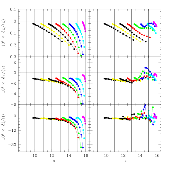
Figure 3: Comparison between two numerical experiments, employing a uniform grid (left) and two levels of refinement (right), in terms of error in the particle position (top), velocity (middle) and force (bottom). The initial set up includes 32 grid cells (bound by vertical lines) and 32 particles uniformly distributed. Only one quarter of the grid is shown, focusing on the critical region where the caustic forms. Vertical lines indicate cells’ boundaries.

The $L_{1}$ and $L_{\infty}$ error norms and convergence rates for the AMR runs are reported on the right hand side of Table 3 while the $L-2$ errors are shown as spur symbols in the left hand side panels of Fig. 2. These results show that employing AMR during the nonlinear evolution improves the convergence rate of the solution in such a way that they resemble the values in the linear stage. This is true in this example for the errors in the position and velocity and to a lesser extent, the force, which is more affected by coarse/fine boundary effects.

Fig. 3 compares the errors in position, velocity and force for a fixed grid (left) and an AMR grid (right) calculations. It focuses on the region where, and the times when, the caustic forms and AMR operates. Thus only one quarter of the total grid is shown (with the cell boundaries of the base grid indicated by vertical lines and marked by integer labels), and the various errors are plotted only for the last one third of the simulation run. At the beginning of that time span (when $a\sim 0.2$), the particles have clustered sufficiently at the grid center and a first level of refinement is created.

Figure 4: Same as Fig. 1 but for the case in which a staggered scheme is used for the force calculation.

Six grid meshes are refined (only three between boundaries, 12-16, are shown in Fig. 3). The second level of refinement is created much later and only affects one base (or two refined) grid mesh(es) for the last ten per cent of the simulation. Fig. 3 shows that the errors in position, velocity and force of the particles close to the point where the caustic forms are much reduced when AMR is employed. The generation of a level of refinement is accompanied by a change in the mass distribution and the potential field. When this happens, a particle may experience a sudden change in terms of the force field acting upon it. These effects are responsible for the somewhat ‘errant’ behavior of the force error, as illustrated in the bottom-left panel of Fig. 3. Overall, though, for each particle the force fluctuations in the AMR case are significantly smaller than the force errors in the uniform grid case.

As a last result for this section, in Fig. 4 we plot $L_{2}$ convergence errors analogous to Fig. 1 but for the case in which the force was computed with a staggered scheme. Comparison of the two figures shows that when $N_{\rm part}=N_{\rm cell}$ the solution obtained with the staggered scheme also converges with second order accuracy, while being characterized by smaller errors. This is in agreement with previous findings [44]. However, when the number of particles is halved ($N_{\rm part}=\frac{1}{2}N_{\rm cell}$) the results obtained with a staggered force scheme worsen more dramatically than for the cell centered case, showing a very poor convergence rate. Closer inspection shows that when the particles are sparse on the grid, oscillations appear in the potential due to the discrete character of the matter distribution as reproduced on the grid. Since this affects only the quality of the staggered scheme the problem may be related to the inconsistency of this scheme with the centering of the stencil used for the discretization of the Laplacian operator. We shall return to this issue in the next test case where the problem reappears with more dramatic effects.

4.1.2 Collisional Component

We now turn to the performance of the hydrodynamic part of the code. We use the same tests employed in the previous section for the the collisionless component. However, since in this case the solution refers to an Eulerian grid, in order to have the velocity and density at a given grid location $x(q,t)$ from Eq. (78)-(79) we must invert Eq. (77).

Table 4: Convergence tests: Godunov’s scheme^†

$N_{\rm part}$	$L_{1}$	$R_{1}$	$L_{2}$	$R_{2}$	$L_{\infty}$	$R_{\infty}$
density
8	2.7e-05	2.2	2.9e-05	1.9	4.2e-05	1.2
16	5.7e-06	2.2	7.6e-06	2.2	1.8e-05	1.8
32	1.2e-06	2.0	1.7e-06	2.2	5.3e-06	1.9
64	3.0e-07	2.0	3.8e-07	2.1	1.4e-06	1.9
128	7.4e-08	–	8.8e-08	–	3.7e-07	–
velocity
8	3.3e-05	2.0	3.6e-05	2.0	5.2e-05	2.0
16	8.1e-06	2.0	9.0e-06	2.0	1.3e-05	2.0
32	2.0e-06	2.0	2.2e-06	2.0	3.2e-06	2.0
64	5.0e-07	2.0	5.6e-07	2.0	7.9e-07	2.0
128	1.2e-07	–	1.4e-07	–	2.0e-07	–
force
8	1.6e-02	2.0	1.7e-02	2.0	2.4e-02	2.0
16	3.9e-03	2.0	4.3e-03	2.0	6.1e-03	2.0
32	9.7e-04	2.0	1.1e-03	2.0	1.5e-03	2.0
64	2.4e-04	2.0	2.7e-04	2.0	3.8e-04	2.0
128	6.0e-05	–	6.7e-05	–	9.5e-05	–

^† We use a cell-centered force scheme and a constant timestep,$\frac{\Delta t}{\Delta x}=1.6\times 10^{-4}$.

We first consider the errors in the linear regime, in analogy to Table 1 and Table 2 for the collisionless component. In Table 4 we report the $L_{1},~{}L_{2}$ and $L_{\infty}$ norms of the error for the gas density, velocity and force and the corresponding convergence rates, for the case of fixed time step, $\frac{\Delta t}{\Delta x}=1.6\times 10^{-4}$. Similarly, the left hand side of Table 5 reports the $L_{1},~{}L_{2}$ and $L_{\infty}$ errors for the case in which the time step is set by the background expansion rate. The $L_{2}$ errors for the fixed and varying timestep cases are also shown by the filled symbols in the left and right hand side panels of Fig. 5, respectively. These tests show the second order accuracy of the implemented scheme. We note, however, that in the case of variable time step the convergence rate of the $L_{\infty}$ norm of the density error is slower.

Table 5: Convergence tests: Godunov’s scheme, linear regime^†

$N_{\rm part}$	$L_{1}$	$R_{1}$	$L_{2}$	$R_{2}$	$L_{\infty}$	$R_{\infty}$
density
8	2.0e-04	2.2	2.1e-04	1.9	3.0e-04	1.1
16	4.2e-05	2.1	5.7e-05	2.1	1.4e-04	1.7
32	9.5e-06	2.0	1.3e-05	1.9	4.3e-05	1.4
64	2.4e-06	1.9	3.5e-06	1.5	1.6e-05	0.9
128	6.5e-07	–	1.3e-06	–	8.4e-06	–
velocity
8	2.1e-04	2.0	2.3e-04	2.0	3.3e-04	2.0
16	5.1e-05	2.0	5.7e-05	2.0	8.2e-05	2.0
32	1.3e-05	2.0	1.4e-05	2.0	2.0e-05	2.1
64	3.2e-06	2.0	3.5e-06	2.0	5.0e-06	1.9
128	7.9e-07	–	8.9e-07	–	1.3e-06	–
force
8	1.5e-02	2.0	1.7e-02	2.1	2.3e-02	2.0
16	3.6e-03	2.0	4.0e-03	2.0	5.7e-03	2.0
32	9.0e-04	2.0	1.0e-04	2.0	1.4e-03	2.0
64	2.2e-04	2.0	2.5e-04	2.0	3.5e-04	2.0
128	5.6e-05	–	6.2e-05	–	8.9e-05	–

^† We use a cell-centered force scheme, a variable timestep, $\frac{\Delta t}{\Delta x}=C_{exp}(\frac{a}{\dot{a}}),~{}C_{exp}=10^{-2}$, and $a=0.0221$.

Table 6: Convergence tests: Godunov’s scheme, nonlinear regime^†

	uniform grid				AMR
$N_{\rm part}$	$L_{1}$	$R_{1}$	$L_{\infty}$	$R_{\infty}$	$L_{1}$	$R_{1}$	$L_{\infty}$	$R_{\infty}$	$l_{max}$
	density
8	2.2e-01	0.5	8.2e-01	–	1.6e-01	0.7	8.2e-01	–	1
16	1.6e-01	0.7	1.2e00	–	1.0e-01	0.6	1.5e00	–	1
32	9.7e-02	0.9	1.5e00	0.0	6.4e-02	2.0	2.4e00	1.3	2
64	5.0e-02	1.6	1.5e00	1.0	1.6e-02	2.0	1.0e00	1.1	2
128	1.6e-02	–	7.3e-01	–	3.9e-03	–	4.7e-01	–	3
	velocity
8	2.7e-02	1.4	9.4e-02	0.4	1.6e-02	1.8	8.6e-02	0.7	1
16	1.0e-02	1.4	7.0e-02	0.4	4.7e-03	1.7	5.3e-02	0.6	1
32	3.8e-03	1.5	5.3e-02	0.6	1.4e-03	2.4	3.6e-02	2.2	2
64	1.3e-03	1.6	3.6e-02	0.9	2.6e-04	1.8	9.6e-03	1.9	2
128	4.3e-04	–	2.0e-02	–	7.2e-05	–	3.1e-03	–	3
	force
8	6.8e-02	1.6	2.3e-01	0.5	3.7e-02	1.7	2.0e-01	0.9	1
16	2.3e-02	1.5	1.6e-01	0.5	1.1e-02	2.3	1.1e-01	0.8	1
32	8.4e-03	1.5	1.1e-01	0.6	2.2e-03	2.0	6.3e-02	1.7	2
64	2.9e-03	1.6	7.3e-02	0.9	5.5e-04	1.8	1.9e-02	2.2	2
128	9.5e-04	–	3.9e-02	–	1.6e-04	–	4.0e-03	–	3

^† We use a cell-centered force scheme, a variable timestep, $\frac{\Delta t}{\Delta x}=C_{exp}(\frac{a}{\dot{a}}),~{}C_{exp}=10^{-2}$, and $a=0.479$.

Figure 5: $L_{2}$ norm of the error in density (top), velocity (center) and force (bottom) as a function of the number of grid cells. See legend for the meaning of the symbols (UG= Uniform Grid, $a$ is the expansion parameter).

Next, the left hand side of Table 6 reports the errors and convergence rates for the case of a uniform grid calculation, well in the nonlinear regime, close the formation of the caustic ($a=0.479$). As before, the $L_{2}$ errors are also shown as open symbols in Fig. 5. Unlike the collisionless case, here is the convergence rate of the density that is mostly affected, particularly at low resolutions (cf. [31, 45]). As illustrated by the $L_{\infty}$ norm, the error is dominated by the contribution of a few cells, located where the caustic forms.

Finally, we test the performance of the AMR code. As for the collisionless component, we use a constant refinement ratio, $n_{\rm ref}=2$, refine cells enclosing a mass larger than 1.5 the average value and allow for a max of three levels of refinement. The results at $a=0.476$ are reported in the right hand side columns of Table 6 for the $L_{1},~{}L_{\infty}$ errors and convergence rates. There we also show the maximum level employed by each run. $L_{2}$ errors are reported as spur symbols in the right panels of Fig. 5.

The use of refined grids in terms of fraction of grid covered and fraction of the simulation time is very similar to the corresponding collisionless case. Similar is also the benefit of AMR, which improves the convergence of the solution to rates very similar to those characterizing the linear regime. This is indeed a powerful performance of the AMR technique.

4.2 Effect of $C_{exp}$ on the Solution Quality

We have investigated how the error depends on the choice of the parameter $C_{exp}$ for the above problem. In particular we have computed the error accumulated during an interval $\Delta a\ll a_{collapse}$, for values of the expansion parameter $a=0.196$ and $a=0.091$, and for values of $C_{exp}$ ranging from $10^{-3}$ to $0.5$. We consider both the fluid and the collisionless case. We use a uniform grid with 32 zones on a side and, for the collisionless case, we use one particle per cell. The results are rather independent of the norm type. We find that the errors introduced in the particles velocity and position is quite stable, except for the largest values of $C_{exp}$. On the other hand, the errors in the fluid components decrease steadily as $C_{exp}$ is reduced, spanning a factor $\sim 5$ before reaching a plateau for $C_{exp}\leq(1-2)\times 10^{-2}$.

4.3 Homologous Dust Cloud Spherical Collapse

In this section we test the ability of the code to follow the collapse of a pressure-less (dust) sphere of matter [46]. The problem is described by the following equations

$$\left(\frac{\partial^{2}r}{\partial t^{2}}\right)_{M} = -G\frac{M(r)}{r^{2}}$$ (80)

$$u = \left(\frac{\partial r}{\partial t}\right)_{M}$$ (81)

with initial conditions

$$\rho({\bf i},t=0) = \left\{\begin{array}[]{lll}f[r({\bf i})]&\mbox{if}&r({\bf i})\leq R\\ 0&\mbox{if}&r({\bf i})>R\end{array}\right.$$ (84)

$$u({\bf i},t=0) = 0$$ (85)

where $M(r)$ is the mass enclosed within a distance $r$ from the sphere center, $R$ is the radius of the sphere and $f(r)$ is a function (with $f^{\prime}(r)\leq 0$) that depends solely on $r$. For the hydrodynamic case null density will be approximated with a value $\rho(r>R)\ll\min[\rho(r)]$. The problem admits a self similar solution in implicit form which reads

$$(1-\xi)^{1/2}\,\xi^{1/2}+\sin^{-1}(1-\xi)^{1/2}=\tau$$ (86)

$$r=\xi\,r_{0},~{}~{}~{}u=\frac{r_{0}}{\tau_{c}}\,\left(\xi^{-1}-1\right)^{1/2},~{}~{}~{}\tau\equiv t\,\left(\frac{8\pi G\langle\rho\rangle_{r}}{3}\right)^{1/2}$$ (87)

where $\langle\rho\rangle_{r}=3M(r)/4\pi r^{3}$ is the average density within a radius $r$.

From the numerical point of view, the problem is challenging in two respects: during collapse the force potential becomes progressively steeper and, therefore, more demanding for the gravity solver. In addition, since the problem has inherent radial symmetry and we are solving it on a Cartesian grid, the ability of the code at preserving that symmetry will be tested.

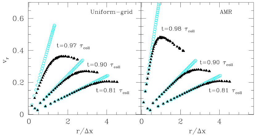
Figure 6: Phase space distribution of particles for the spherical collapse of a pressureless cloud. Cyan open circles correspond to the analytic solution and filled triangles to the numerical simulation result. The right panel is for the case of a uniform grid whereas the left panel correspond to an AMR calculation with two levels of refinement.

For the collisionless component we initially set particles with null velocity at the center of cells whose distance from the cloud center is less than $R$ (=1). This produces a homogeneous density distribution everywhere inside R, except close to the cloud edge due to the discreteness of the grid. In Fig. 6 we compare the position of each particle in phase-space ($v_{r},r$) as given by the code (black filled triangles) with the analytic solution (cyan open circle). The left panel corresponds to the case in which a uniform grid is used whereas for the right panel solution AMR was employed. We allow for two levels of refinement and tag cells with a total mass four times as high as the initial value. The comparison between analytic and numerical solution in Fig. 6 is made for a number of evolution times, expressed in terms of the adimensional collapse time $\tau_{coll}=\pi/2$. Noticeably, the code follows the particles motions with high accuracy all the way down to the time of collapse. In particular, there is no sign of artificial asymmetries. Additional levels of refinement were dynamically generated towards the final phase of the collapse. At the latest time shown ($\tau=0.98\,\tau_{coll}$), we can see the improvement due to the employment of finer grids in the collapsing region. Note that towards the edge of the cloud the particles are trailing. This is due to the inability to reproduce a perfectly homogeneous sphere near the cloud edge from the beginning. The region affected by this is about one mesh size wide.

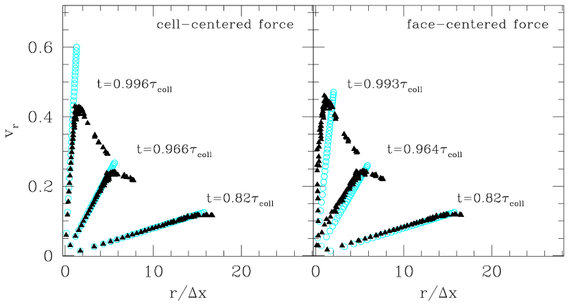
Figure 7: Phase space distribution of particles for the spherical collapse of a pressureless cloud. The initial cell-to-particle ratio is 4. Cyan open circles correspond to the analytic solution and filled triangles to the numerical simulation result using a cell-centered (left) and face-centered (right) force scheme, respectively.

When exploring the accuracy of cell-centered versus face-centered force schemes our tests suggest that, again, in the uniform grid case the latter perform slightly better, at the level of ca 15%. In analogy with the analysis of Sec. 4.1, we have tested this further, for the case in which the ratio of cells to particles is significantly larger than one. This situation may easily occur depending on the adopted criterion for refinement and on the efficiency for the generation of the refined grid out of the tagged cells. In Fig. 7 we compare the solutions obtained with a cell-centered (left) and a staggered (right) force scheme for an initial cell-to-particle ratio of 4. The initial dust sphere is placed on a grid of 256 cells on a side, and 8 particles are aligned along its radius out to 32 cells from its center. The code output is plotted at three different solution times close to the time of collapse $t=\tau_{coll}$. This test shows that when the number of cell-to-particle ratio is significantly higher than one, the staggered force scheme tends to produce spurious results. This is in line with the findings in the previous test problem in section 4.1. On the other hand, the cell-centered scheme seems well behaved. We find that the qualitative result does not change when we use a two or four point force stencil, when the number of particles to resolve the sphere is changed or when the sphere center is shifted by a fraction of a mesh size in an arbitrary direction.

Thus the staggered force scheme, although apparently more accurate than its cell-centered counterpart when the number of cells is comparable to, or less than, the number of particles [44], it gives rise to spurious results when particles are sparse on the grid. Therefore, caution must be exercised when employing staggered schemes for force evaluation.

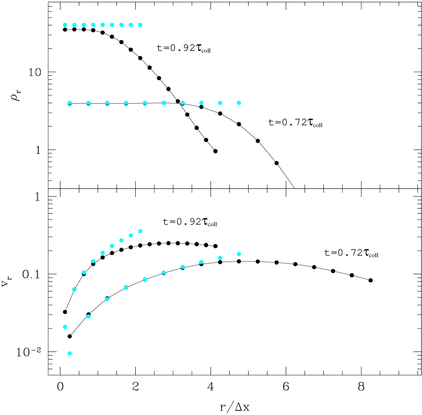
Figure 8: Density and velocity profile for spherical collapse of a pressureless cloud of gas. Cyan open circles correspond to the analytic solution and black filled dots to the numerical simulation results.

Finally, the results for the collisional case are illustrated in Fig. 8. The plot compares the density (top) and velocity (bottom) profiles of the numerical solution (threaded black dots) and the analytic solution (cyan dots). The latter extend only out the cloud size, whereas the numerical solution includes the region covered by the finest level. Two times during the collapse are shown: $t=0.72\tau_{coll}$ and $t=0.92\tau_{coll}$, corresponding to the low and high curves, respectively. At these times one and two levels of refinement have been generated, respectively. The chosen times are close to the collapse time, when the errors have accumulated and the simulation becomes more challenging. Nevertheless, as for the collisionless component, the code follows accurately the evolution of the density and velocity profiles of the collapsing cloud. Again, close to the cloud edge the density profile is smoother and the velocity field slower than the analytic solution. The size of the region affected by this is again of order of the coarse mesh size and it is partially ascribed to the crude representation of the cloud edge on the grid.

4.4 Energy Conservation: Layzer-Irvine Equation

For pure hydrodynamics conservation of the total (kinetic+thermal) energy is enforced by our conservative Godunov’s method. When gravity is added, energy conservation should still hold, but is not explicitly enforced in our scheme. Finally, with an expanding background energy is not conserved. For a collection of particles that interact only gravitationally, the evolution of the energy of the system is regulated by the Layzer-Irvine equation, which reads

$$\frac{d}{dt}[a(t)({\cal E+W})]=-\dot{a}\,{\cal E}$$ (88)

where ${\cal E}$ is the kinetic energy associated to the peculiar motions of the particles and ${\cal W}$ their gravitational potential energy due to the overdensity produced by their mass distribution. Clearly in absence of expansion ($a=1$, $\dot{a}=0$) Eq. (88) reduces to the ordinary energy conservation equation. Otherwise it describes the change in the total energy of the system due to the adiabatic expansion of the background. The derivation and physical meaning of Eq. (88) is reviewed in Ref. [27]. Its applicability to hydrodynamic simulations is discussed in, e.g., Ref. [32], in which case a monoatomic gas is assumed and ${\cal E}$ includes both the kinetic and thermal energy of the gas.

Eq. (88) can be integrated in time giving

$$a[{\cal E}(a)+{\cal W}(a)]-a_{0}[{\cal E}(a_{0})+{\cal W}(a_{0})]=-\int_{a_{0}}^{a}{\cal E}da.$$ (89)

We can evaluate the integral on the RHS of the above equation numerically with the trapezoidal rule and assess the accuracy of the code at tracking the energy of the system through the quantity

$$\delta\varepsilon=\frac{a[{\cal E}(a)+{\cal W}(a)]-a_{0}[{\cal E}(a_{0})+{\cal W}(a_{0})]+\int_{a_{0}}^{a}{\cal E}da}{[a_{0}{\cal W}(a_{0})-a{\cal W}(a)]}.$$ (90)

Figure 9: Energy conservation error based on Eq.(90) for the collapse of a pressureless spherical cloud (left) and a cosmological run (right). See text for details.

We first test the energy conservation accuracy of the code for the case of the collapse of a pressureless cloud. This is the problem studied in the previous section. We carry out three AMR calculation with different base grid sizes, namely 16, 32, 64 corresponding to 4, 8, 16 cells per cloud radius respectively. In these runs, cells enclosing more then four times the initial mass content were tagged for refinement and a maximum of two 2 refinement levels were allowed. The results of the test are reported in the left hand side panel of Fig. 9 where we plot the error in the total energy, $\delta\varepsilon$, as a function of resolution, for both the particle (open) and the gasdynamic (filled) case. The plots show that with 16 zones per cloud radius the error in the energy is at the level of a per cent or so.

Next we test code accuracy at tracking the energy of the system in a cosmological run. For the purpose we use a $\Lambda$-Cold Dark Matter cosmology with parameters $\Omega_{m}$=0.3, $\Omega_{\Lambda}=0.7$, $\Omega_{b}$ = 0.04, for the energy density in total matter, dark energy and baryonic matter respectively; and $H_{0}=70$ km s^-1 Mpc^-1 for the Hubble constant. The physical domain has a size of L=91.43 Mpc on a side. We execute three runs with different numerical resolution. The first two runs employ a uniform grid with 32³ and 64³ cells, respectively, and the same number of particles as grid cells. The third run uses a base grid with 32³ cells and 32³ particles, and two additional levels of refinement created in region where the total mass enclosed in a cell exceeds the initial value by a factor eigth. The initial conditions where generated on a 64³ grid and coarse-averaged to a 32³ grid for the low-resolution-uniform and AMR runs.

The results are presented in the right panel of Fig. 9 where we plot $\delta\varepsilon$ (top), ${\cal E}$ (middle) and ${\cal W}$ (bottom) as a function of expansion parameter $a$ for each resolution case. The plots show that when using a uniform grid the total energy of the system is evolved with an accuracy at the percent level ($\sim$ 2% and 1% for the $32^{3}$ (dot) and $64^{3}$ (dash) cases, respectively), with most of the error generated at startup. In the AMR case (solid line), however, our error parameter $\delta\varepsilon$ increases visibly when refinement levels are created (at $a\sim 0.15$ and $a\sim 0.2$ for the first and second level respectively). The reason for this is simple. When a level of refinement is created the potential energy of the system changes suddenly (see solid and dot lines in the bottom panel) throwing off the balance bewtween particle/gas velocities and their potential energy. As a result a large error in the sense of Eq.(90) is generated. This is so, even though with the additional level of refinement the potential energy of the system is more accurate as it gets closer the value from the high resolution run (see solid and dash lines in the bottom panel). Over time the kinetic energy readjusts to the new potential (middle panel; notice that the internal energy is negligible) and a balance between the two forms of energy is reestablished. Because the potential energy associated with the newly formed structures is larger than that of the system at the time when the refinement levels were first generated, the new balance between kinetic and potential energy reduces substantially the error as time progresses. At simulation end the AMR run (with a base grid of $32^{3}$ cells) produces estimates of $\delta\varepsilon$, ${\cal E}$ and ${\cal W}$ very close to the high resolution run.

4.5 Santa Barbara Galaxy Cluster

In this section we carry out the calculation defined by the ‘Santa Barbara Cluster Comparison Project’ [47] and compare the results of our code with those from different codes implemented independently by other authors and based either on similar or different techniques.

The problem consists of simulating the formation of a galaxy cluster in a Standard Cold Dark Matter universe. The cosmological parameters assumed were $\Omega_{m}$= 1 and $\Omega_{b}$ = 0.1 for the total and baryonic mean mass density in units of the critical density, respectively; $H_{0}=50$ km s^-1 Mpc^-1 for the Hubble constant; $\sigma_{8}$ = 0.9 for the present-day linear rms mass fluctuation in spherical top hat spheres of radius 16 Mpc; for the baryon density. The computational domain has a size of L=64 Mpc on a side. The initial matter fluctuation are characterized by a power spectrum with an asymptotic spectral index, n = 1, and are ‘constrained’ so that at simulation end a massive structure has formed at the center of the computational box.

The simulation was initialized at z = 40 with two grids already in place: a base grid covering the entire 64 Mpc³ domain with 64³ cells and 64³ particles; and a second grid, also with 64³ cells and 64³ particles, but only 32 Mpc on a side and placed in the central region of the base grid, thus yielding an initial cell size of 0.5 Mpc. Refinement is applied only in this central, higher resolution region and is based on a local density criterion: cells with a total mass of $6.4\times 10^{10}$ M_⊙ or more were refined. We allowed for 5 levels of refinement (for a total of a 6 levels hierarchy), with a constant refinement ratio $n_{ref}=2$. The size of the finest mesh is about 15 comoving kpc. We use the following CFL coefficients for the time step: $C_{\rm hydro}=0.8,~{}C_{\rm part}=0.5$ and $C_{\rm exp}=0.02$.

At simulation end a halo finder based on the spherical overdensity method [48] was run in order to define the center of the galaxy cluster. The radial profiles for six quantities of interest are presented in Fig. 10 together with results from two other simulation codes: ENZO, which is an Eulerian AMR code similar to ours, and HYDRA (as run by Jenkins & Pearce), which combines smoothed particle hydrodynamics (SPH) and adaptive particle-particle-particle-mesh (AP³M) method for the N-body part [49]. These two codes are meant to be representative of the high resolution grid based and SPH approaches, respectively.

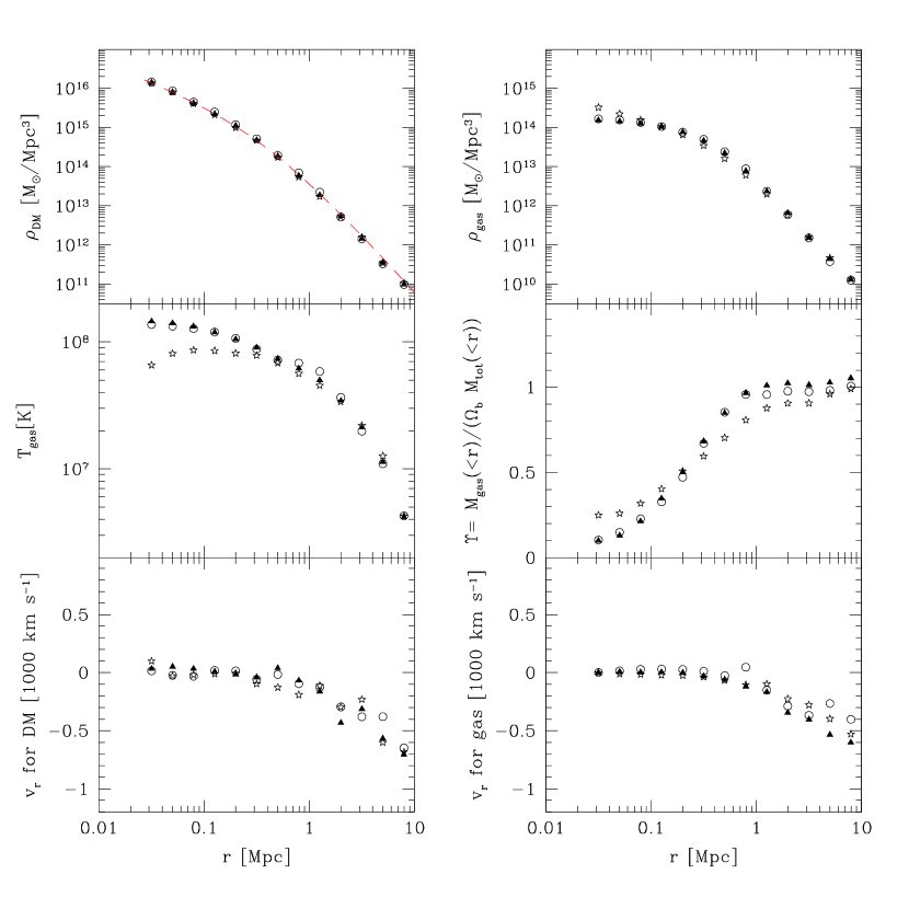
Figure 10: Radial profile of dark matter (top left), baryonic gas (top right) temperature (middle left), baryonic fraction (middle right), radial velocity for dark matter (bottom left) and gas (bottom right). In addition to the results from CHARM (open dots), for comparison we also show those from the ENZO AMR code (filled triangles) [21] as well as those from the HYDRA SPH code (open stars) [49].

Results are shown down to scales of about 30 kpc which is just above the nominal resolution at finest level of refinement. The plot shows that there is good agreement among the results of the different codes particularly with ENZO (even though we used one less level of refinement and use a different refinement criterion). The discrepancies, when significant, are consistent with those already found in the extensive comparison paper in Ref. [47]. In fact, there is very good agreement in terms of dark matter density distribution (top left) which is well fit by the analytical form proposed in Ref. [50] with parameters specified in the caption. Similarly, there is good matching of the solution in terms of gas density distribution, except in the inner regions within 100 kpc, where the two AMR solutions flattens and the SPH solution keeps on increasing. More significant is the difference in temperature distribution (middle left), which drops in the SPH solution for the inner regions and stays constant for the AMR case. These differences were already found and discussed in Ref. [47]. (See also Ref. [19] for similar findings.) Their origin is not fully clear, although as suggested in Ref. [47], it could be ascribed to the different way in which SPH and grid based methods treat shocks.

Next panel (middle right) shows the profile for the ratio of gas to dark matter mass, normalized to the global value. While our solution is in good agreement with ENZO’s and deviates from HYDRA’s in the inner regions and is somewhat in between the two beyond 1 Mpc or so. There is significant scatter in the results from the full set of codes found in Ref. [47], at the level of 0.1-0.2. Nevertheless, it is pointed out in Ref. [47] that when integrated out to the virial radius of the system (2.7 Mpc), the SPH codes seem to predict a systematically slightly smaller values for this quantity than high resolution grid based codes. The reason for this is still not clear.

Finally, both the gas and dark matter radial velocity profiles agree quite well at all radii. Some differences may arise due to slight differences in the simulation timing, as pointed out in Ref. [47]. Note that at larger radii (last few points), typically characterized by wider scatter, both ENZO’s and HYDRA’s results tend to be below the average value defined in Ref. [47].

5 Conclusions

We have presented a new code based on AMR technique for systems comprising collisional and collisionless components coupled through a long range force. We have thus extended the scheme in [2] to include collisionless particle dynamics and gravity arising from the mass distribution of the two components. For the hydrodynamics we use a slightly modified directionally unsplit Godunov’s method based on Ref. [28]. As for the collisionless component we have implemented various time centered modified symplectic schemes based on both the kick-drift-kick and drift-kick-drift sequence. Our implementations of these schemes appear to perform comparably. We have also used several types of stencil to calculate the force from the potential. We find that while the staggered schemes appear more accurate when the number (density) of particles is at least as large as the number of grid cells, it produces spurious results when the particles are sparse on the grid. Cell centered stencils thus seem more reliable, especially when a five point cell centered discretization of the Laplacian operator is used.

Due to the time refinement character of the AMR technique the solution on different levels is advanced with different timesteps. Synchronization issues then arise as the multilevel solution to the elliptic equation needs to be solved simultaneously on all levels. In particular, the density field represented by the particles evolved on finer levels may not be available on coarser levels when they are not synchronized. Similarly, one cannot account for the effects of the mass distribution on finer levels on the multilevel solution of the potential, unless all levels are synchronized. Among other features of the code, we have thus introduced an aggregation procedure to cost-effectively represent on the coarser levels the particles on finer levels without compromising the code accuracy and performance. We have also implemented a procedure for estimating (when the coarse and finer levels are not synchronized) the effects on the coarse potential produced by the matching conditions at refinement boundaries between coarse and fine solution, as they would arise in a full multilevel calculation. We performed several standard tests which illustrate the code accuracy as well as the advantages of the AMR technique for the study of both self gravitating hyperbolic systems, collisionless system and hybrid systems.

FM is thankful to D. Serafini, D. Martin, B. van Straalen and D. Graves for useful discussions, to the Lawrence Berkeley National Laboratory, for its hospitality, to the Institute of Informatics, ETH Zürich, for technical support. FM also acknowledges partial support by the European Community through contract HPRN-CT2000-00126 RG29185 and by the Swiss Institute of Technology through a Zwicky Prize Fellowship.

Charge Assignment Schemes

Indicating with $\Delta x$ the mesh size in one dimension we find the nearest grid point scheme (NGP) defined for order $r=1$ as

$$W(\hat{x}-x)=\left\{\begin{array}[]{ll}1&~{}~{}~{}~{}~{}~{}~{}~{}~{}{\rm if}~{}~{}|\hat{x}-x|\leq\Delta x/2\\ 0&~{}~{}~{}~{}~{}~{}~{}~{}~{}{\rm otherwise}\end{array}\right.$$ (91)

in which the assigned charge distribution is discontinuous as the particle cross the cell boundary; the cloud in cell (CIC) scheme defined for $r=2$ as

$$W(\hat{x}-x)=\left\{\begin{array}[]{ll}1-\frac{|\hat{x}-x|}{\Delta x}~{}~{}{\rm if{}{}}&|\hat{x}-x|\leq\Delta x\\ 0&~{}~{}{\rm otherwise}\end{array}\right.$$ (92)

in which the assigned charge distribution is continuous but the first derivative is not; the cell boundary; and the triangular shape cloud (TSC) scheme defined for $r=3$ as

$$W(\hat{x}-x)=\left\{\begin{array}[]{ll}\frac{3}{4}-\left(\frac{|\hat{x}-x|}{\Delta x}\right)^{2}&~{}~{}~{}~{}~{}~{}~{}~{}~{}{\rm if}~{}~{}|\hat{x}-x|\leq\Delta x/2\\ \frac{1}{2}-\left(\frac{3}{2}-\frac{|\hat{x}-x|}{\Delta x}\right)^{2}&~{}~{}~{}~{}~{}~{}~{}~{}~{}{\rm if}~{}~{}\Delta x/2\leq|\hat{x}-x|\leq 3\Delta x/2\\ 0&~{}~{}~{}~{}~{}~{}~{}~{}~{}{\rm otherwise}\end{array}\right.$$ (93)

in which both the assigned charge distribution and first derivative are continuous. These schemes retain their properties when they are extended to a multidimensional case in the form of a product

$$W({\bf\hat{x}}-{\bf x})=\prod_{j=1}^{D}W_{j}(\hat{x}_{j}-x_{j}).$$ (94)

References

- [1] M. J. Berger, Oliger, Adaptive mesh refinement for hyperbolic partial differential equations, J. Comp. Phys. 53 (1984) 484–512.
- [2] M. J. Berger, P. Colella, Local adaptive mesh refinement for shock hydrodynamics, J. Comp. Phys. 82 (1989) 64–84.
- [3] F. X. Timmes, M. Zingale, K. Olson, B. Fryxell, P. Ricker, A. C. Calder, L. J. Dursi, H. Tufo, P. MacNeice, J. W. Truran, R. Rosner, On the Cellular Structure of Carbon Detonations, Astrophys. J. 543 (2000) 938–954.
- [4] K. Kifonidis, T. Plewa, H.-T. Janka, E. Müller, Nucleosynthesis and Clump Formation in a Core-Collapse Supernova, Astrophys. J. Lett. 531 (2000) L123–L126.
- [5] A. S. Almgren, J. B. Bell, C. A. Rendelman, M. Zingale, Low Mach number modeling of type Ia supernovae. I. hydrodynamics, Astrophys. J. 637 (2006) 922–936.
- [6] A. S. Almgren, J. B. Bell, C. A. Rendelman, M. Zingale, Low Mach number modeling of type Ia supernovae. II. energy evolution, Astrophys. J. in press.
- [7] R. I. Klein, C. F. McKee, P. Colella, On the hydrodynamic interaction of shock waves with interstellar clouds. 1: Nonradiative shocks in small clouds, Astrophys. J. 420 (1994) 213–236.
- [8] R. Walder, D. Folini, Knots, filaments, and turbulence in radiative shocks, Astr. Astrophys. 330 (1998) L21–L24.
- [9] R. I. Klein, R. T. Fisher, M. R. Krumholz, C. F. McKee, Recent Advances in the Collapse and Fragmentation of Turbulent Molecular Cloud Cores, in: Revista Mexicana de Astronomia y Astrofisica Conference Series, 2003, pp. 92–96.
- [10] J. K. Truelove, R. I. Klein, C. F. McKee, J. H. Holliman, L. H. Howell, J. A. Greenough, The Jeans Condition: A New Constraint on Spatial Resolution in Simulations of Isothermal Self-gravitational Hydrodynamics, Astrophys. J. Lett. 489 (1997) L179+.
- [11] J. K. Truelove, R. I. Klein, C. F. McKee, J. H. Holliman, L. H. Howell, J. A. Greenough, D. T. Woods, Self-gravitational Hydrodynamics with Three-dimensional Adaptive Mesh Refinement: Methodology and Applications to Molecular Cloud Collapse and Fragmentation, Astrophys. J. 495 (1998) 821–+.
- [12] T. Abel, G. L. Bryan, M. L. Norman, The Formation of the First Star in the Universe, Science 295 (2002) 93–98.
- [13] M. L. Norman, Cosmological Simulations of X-ray Clusters: The Quest for Higher Resolution and Essential Physics, ArXiv Astrophysics e-prints.
- [14] D. F. Martin, K. L. Cartwright, Solving Poisson’s equation using adaptive mesh refinement, Technical Report UCB/ERI M96/66 UC Berkeley.
- [15] P. M. Ricker, K. Olson, K. M. Riley, F. Miniati, et al., Adding self-gravitation and collisionless particles to an adaptive-mesh hydrodynamics codeIn prep.
- [16] A. V. Kravtsov, High-resolution simulations of structure formation in the universe, Ph.D. Thesis.
- [17] A. Knebe, A. Green, J. Binney, Multi-level adaptive particle mesh (MLAPM): a c code for cosmological simulations, Mon. Not. R. Astron. Soc. 325 (2001) 845–864.
- [18] R. Teyssier, Cosmological hydrodynamics with adaptive mesh refinement. A new high resolution code called RAMSES, Astr. Astrophys. 385 (2002) 337–364.
- [19] V. Quilis, A new multidimensional adaptive mesh refinement hydro + gravity cosmological code, Mon. Not. R. Astron. Soc. 352 (2004) 1426–1438.
- [20] R. W. Hockney, J. W. Eastwood, Computer Simulation Using Particles, McGraw Hill, New York, 1981.
- [21] G. L. Bryan, M. L. Norman, A hybrid amr application for cosmology and astrophysics, in: D. A. Clarke, M. Fall (Eds.), Computational Astrophysics, ASP Conference, 1997.
- [22] G. Strang, On the construction and comparison of difference schemes, SIAM J. Num. Anal. 5 (1968) 506–517.
- [23] J. Vay, P. Colella, P. McCorquodale, B. V. Straalen, A. Friedman, D. Grote, Mesh refinement for particle-in-cell plasma simulations: Applications to and benefits for heavy ion fusion, Laser & Particle Beams 20 (4) (2002) 596–75.
- [24] G. H. Miller, P. Colella, A conservative three-dimensional eulerian method for coupled solid-fluid shock capturing, J. Comp. Phys. 183 (1) (2002) 26–82.
- [25] A. Almgren, J. Bell, P. Colella, L. Howell, M. Welcome, A conservative adaptive projection method for the variable density incompressible Navier-Stokes equations, J. Comput. Phys. 142 (1998) 1–46.
- [26] D. Martin, P. Colella, A cell-centered adaptive projection method for the incompressible Euler equations, J. Comput. Phys. 163 (2000) 271–312.
- [27] P. J. E. Peebles, Principles of Physical Cosmology, Princeton University Press, Princeton New Jersey, 1993.
- [28] P. Colella, Multidimensional upwind methods for hyperbolic conservation laws, J. Comp. Phys. 82 (1989) 64–84.
- [29] J. Saltzman, An Unsplit 3D Upwind Method for Hyperbolic Conservation Laws, Journal of Computational Physics 115 (1994) 153–168.
- [30] F. Miniati, D. Ryu, H. Kang, T. W. Jones, R. Cen, J. Ostriker, Properties of cosmic shock waves in large-scale structure formation, Astrophys. J. 542 (2000) 608–621.
- [31] G. L. Bryan, M. L. Norman, J. M. Stone, R. Cen, J. P. Ostriker, A piecewise parabolic method for cosmological hydrodynamics, Comp. Phys. Comm. 89 (1995) 149–168.
- [32] D. Ryu, J. P. Ostriker, H. Kang, R. Cen, A cosmological hydrodynamic code based on the total variation diminishing scheme, Astrophys. J. 414 (1993) 1.
- [33] T. Quinn, N. Katz, J. Stadel, G. Lake, Time stepping N-body simulations; e-archive: astro-ph/9710043.
- [34] W. Kahan, R.-C. Li, Unconventional Schemes for a Class of Ordinary Differential Equations– with Applications to the Korteweg-de Vries Equation, J. Comp. Phys. 134 (2) (1997) 316–331.
- [35] R. J. LeVeque, Numerical Methods for Conservative Laws, 2nd Edition, Springer, Verlag, 1992.
- [36] M. Minion, A projection method for locally refined grids, J. Comp. Phys. 127 (1996) 158–178.
- [37] D. F. Martin, P. Colella, D. Graves, A cell-centered adaptive projection method for the incompressible Navier-Stokes equations in three dimensions, J. Comp. Phys. .
- [38] R. T. Fisher, Single and multiple star formation in turbulent molecular cloud cores, Ph.D. thesis, University of California, Berkeley (2002).
- [39] S. L. W. McMillan, S. J. Aarseth, An O(N log N) integration scheme for collisional stellar systems, Astrophys. J. 414 (1993) 200–212.
- [40] F. Miniati, P. Colella, A modified Godunov’s scheme for stiff source conservative hydrodynamics, J. Comp. Phys. 224 (2) (2007) 519–538.
- [41] F. Miniati, COSMOCR: A numerical code for cosmic ray studies in computational cosmology, Comp. Phys. Comm. 141 (2001) 17–38.
- [42] F. Miniati, Glimm-Godunov’s method for cosmic-ray-hydrodynamics, J. Comp. Phys. submitted, eprint arXiv:astro-ph/0611499.
- [43] Y. B. Zel’dovich, Gravitational iinstability: an approximate theory for large density perturbations, Astr. Astrophys. 5 (1970) 84–89.
- [44] A. L. Mellot, Comment on “nonlinear gravitational clustering in cosmology”, Phys. Rev. Lett. 56 (1986) 1992.
- [45] L. Feng, C. Shu, M. Zhang, A Hybrid Cosmological Hydrodynamic/N-Body Code Based on a Weighted Essentially Nonoscillatory Scheme, Astrophys. J. 612 (2004) 1–13.
- [46] S. A. Colgate, R. H. White, The Hydrodynamic Behavior of Supernovae Explosions, Astrophys. J. 143 (1966) 626–+.
- [47] C. S. Frenk, S. D. M. White, P. Bode, J. R. Bond, G. L. Bryan, R. Cen, H. M. P. Couchman, A. E. Evrard, N. Gnedin, A. Jenkins, A. M. Khokhlov, A. Klypin, J. F. Navarro, M. L. Norman, J. P. Ostriker, J. M. Owen, F. R. Pearce, U. L. Pen, M. Steinmetz, P. A. Thomas, J. V. Villumsen, J. W. Wadsley, M. S. Warren, G. Xu, G. Yepes, The santa barbara cluster comparison project: A comparison of cosmological hydrodynamics solutions, Astrophys. J. 525 (1999) 554.
- [48] C. Lacey, S. Cole, Merger rates in hierarchical models of galaxy formation - part two - comparison with n-body simulations, Mon. Not. R. Astron. Soc. 271 (3) (1994) 676.
- [49] H. M. P. Couchman, P. A. Thomas, F. R. Pearce, Hydra: an Adaptive-Mesh Implementation of P 3M-SPH, Astrophys. J. 452 (1995) 797–+.
- [50] J. F. Navarro, C. S. Frenk, S. D. M. White, A universal density profile from hierarchical clustering, Astrophys. J. 490 (1997) 493.