The magnetic Bp star 36 Lyncis
I. Magnetic and photospheric properties

Abstract

Aims. This paper reports the photospheric, magnetic and circumstellar gas characteristics of the magnetic B8p star 36 Lyncis (HD 79158).

Methods. Using archival data and new polarised and unpolarised high-resolution spectra, we redetermine the basic physical properties, the rotational period and the geometry of the magnetic field, and the photospheric abundances of various elements.

Results. Based on magnetic and spectroscopic measurements, we infer an improved rotational period of $3.83475\pm 0.00002$ d. We determine a current epoch of the longitudinal magnetic field positive extremum (HJD 2452246.033), and provide constraints on the geometry of the dipole magnetic field ($i\geq 56\degr$, $3210\leavevmode\nobreak\ {\rm G}\leq B_{\rm d}\leq 3930$ G, $\beta$ unconstrained). We redetermine the effective temperature and surface gravity using the optical and UV energy distributions, optical photometry and Balmer line profiles ($T_{\rm eff}=13300\pm 300$ K, $\log g=3.7-4.2$), and based on the Hipparcos parallax we redetermine the luminosity, mass, radius and true rotational speed ($L=2.54\pm 0.16\leavevmode\nobreak\ L_{\odot},M=4.0\pm 0.2\leavevmode\nobreak\ M_{\odot},R=3.4\pm 0.7\leavevmode\nobreak\ R_{\odot},v_{\rm eq}=45-61.5$ km s^-1). We measure photospheric abundances for 21 elements using optical and UV spectra, and constrain the presence of vertical stratification of these elements. We perform preliminary preliminary Doppler Imaging of the surface distribution of Fe, finding that Fe is distributed in a patchy belt near the rotational equator. Most remarkably, we confirm strong variations of the H$\alpha$ line core which we interpret as due to occultations of the star by magnetically-confined circumstellar gas.

1 Introduction

The magnetic Bp stars exhibit a rich variety of magnetic and wind phenomena, many of which are unique to this class of star. Landstreet & Borra (1978), detecting for the first time a magnetic field in a helium strong star, proposed that the photometric and spectroscopic variations of $\sigma$ Ori E resulted from hot gas trapped above the magnetic equator. Brown et al. (1985) discovered unexpectedly strong C iv, Si iv and N v ultraviolet resonance line absorption and emission that varied with the rotational period of the magnetic helium weak star HD 21699. Subsequent work revealed similar phenomena in a number of other Bp stars, which was attributed to rotational modulation of magnetically-structured stellar winds (e.g. Shore 1987, Shore et al. 1990, Shore & Brown 1990, Bolton 1994, Donati et al. 2001, Smith & Groote 2001, Neiner et al. 2003). The additional discovery of non-thermal radio emission (Drake et al. 1987) from a subset of these objects resulted in the proposal that these stars are surrounded by an extended wind-generated magnetosphere (Linsky et al. 1992), in which the radio luminosity results from optically thick gyrosynchrotron emission and should therefore correlate with both magnetic field strength and effective temperature. According to Drake et al. (2002), by 2002 about 120 magnetic CP stars had been observed in the radio, and of these about 25% had been confidently detected. The general existence of this phenomenon, and the establishment of correlations between effective temperature, magnetic field strength, rotational period and radio emission suggest that this phenomenon is intrinsic to Ap and Bp stars, and is related to their magnetic properties. Subsequently, X-ray emission was discovered (Drake et al. 1994) from a small number of these objects. As pointed out by Drake et al. (2002), no clear correlation of X-ray brightness with other physical or observational characteristics (including radio luminosity) has been established, suggesting (at least in the A-type magnetic stars) that X-ray emission may be due to the presence of late-type companions, and unrelated to their magnetic properties. More recently, sophisticated models describing the hydrodynamic interaction between the magnetic field and wind flow have been developed (Babel & Montmerle 1997, ud-Doula & Owocki 2002, Preuss et al. 2004, Townsend & Owocki 2005), leading to the possibility of combining the various individual kinds of observations (magnetic, radio, optical, UV, X-ray) into a single coherent picture of the wind-magnetic field interaction and subsequent circumstellar structure of magnetic Bp stars.

36 Lyncis (HD 79158) is a bright ($V=5.3$), well-studied magnetic (Borra, Landstreet & Thompson 1983) helium weak B star. It is classified as B8IIIpMn in the Bright Star Catalogue (Hoffleit et al. 1995), as a Si star by Molnar (1972), as a Mn star by Cowley (1972), and as a Sr Ti helium weak star by Borra & Landstreet (1983). It was first identified as peculiar by Edwards (1932). The spectrum and abundances have been studied by Searle & Sargent (1964), Mihalas & Henshaw (1966) and Sargent, Greenstein & Sargent (1969). According to these studies, lines of neutral He and O are weak, whereas those of C, Ne, Si, Mg and Cr are only marginally anomalous. Lines of Ti and Fe are anomalously strong. HD 79158 is a member of the sn class (Abt & Levato 1978), which means its Si ii lines are sharp, whereas He i lines are nebulous. Ryabchikova & Stateva (1995) concluded that 36 Lyn is a classical helium weak star.

Using IUE spectra, Sadakane (1984) reported the presence of strong lines coincident with the position of the C iv $\lambda\lambda 1548,1550$ and Si iv $\lambda\lambda 1394,1403$ resonance doublets. Shore, Brown & Sonneborn (1987) obtained additional magnetic field measurements and IUE spectra of 36 Lyn and two additional sn stars, confirming the presence of the “superionised” C iv and Si iv resonance lines and detecting variability of these features. Shore et al. (1990) extended these observations and analysis, obtaining 22 new measurements of the longitudinal magnetic field and determining a rotational period of $3.8345\pm 0.001$ days.

The goal of the present paper is to provide an accurate reassessment of the magnetic and photospheric properties of 36 Lyn as the basis for a detailed study of properties of the circumstellar matter (Smith et al. 2006, “Paper II”).

2 New and archival observations

2.1 Unpolarised optical spectra

The journal of the unpolarised optical spectroscopic observations is presented in Table 1, available only in electronic form from the CDS.

2.1.1 DAO and DDO Spectra

H$\alpha$ observations of 36 Lyn were obtained at the Dominion Astrophysical Observatory (DAO) with both the 1.85 m Plaskett (1991, 1992, and 1997-2000) and 1.22 m McKellar (2001, 2003-2005) telescopes, and at the David Dunlap Observatory 1.88 m telescope (1992, 1997, and 2004).

At DAO, on the 1.85 m we used the Cassegrain spectrograph with the 21 inch $f/5$ camera, 1800 line mm^-1 grating in first order, VSIS21B image slicer, and various CCDs. The resulting spectra covered a minimum of approximately 100 Å and, when possible, included the He i $\lambda$6678 feature. The dispersion of 10 Å mm^-1 and effective slit width of 40 $\mu$m gave a resolution of approximately $R=16400$.

The 2001 McKellar observations were obtained on the coudé spectrograph with the short camera, 1200 line mm^-1 holographic grating in first order, IS32R image slicer, and the UBC-1 CCD. These short camera observations have a dispersion of 10.1 Å mm^-1 and the resolution is approximately $R=20000$.

For the 2003, 2004 and 2005 McKellar data we again used the coudé spectrograph, but with the long camera, 830 line mm^-1 grating in first order, IS32R image slicer, and the SITe4 CCD with 15 $\mu$m pixels. The dispersion of 4.8 Å mm^-1 and projected slit width of 36 $\mu$m produced a resolution of $R=38000$.

Exposure times on both telescopes ranged from 10 to 30 minutes.

DDO spectra obtained in 1992 and 1997 were recorded with a Thomson 1024$\times$1024 CCD on the Cassegrain spectrograph of the 1.88 m telescope. The effective resolution was ${\rm R}=11600$. Most of the spectra were centered near 6600 Å  so that the 200 Å  range covered by the detector included both H$\alpha$ and the He i $\lambda$6678 Å  line.

The DDO spectra obtained in 2004 were recorded with a Jobin-Yvon 800$\times$2000 thinned, back illuminated CCD with 15 $\mu$m pixels. The effective resolution of these spectra is 14700. These observations were taken in the same way as the earlier observations. However, there were difficulties because the detector system was not operating properly. Due to the large RFI introduced by the heater system and the lack of a cold finger in the dewar, we had to operate the detector system with the temperature floating near the liquid nitrogen vaporization temperature. As a result, there were large changes in the CCD temperature as a function of hour angle of the telescope. To minimize this problem, we took frequent biases, and linearly interpolated in time between them to obtain the bias for each stellar spectrum. The low operating temperature also reduced the dynamic range of the CCD. Flat field exposures showed that the response started to become nonlinear at 24k e^-. As a result, these spectra have somewhat lower S/N than our earlier spectra.

All data were reduced with IRAF in a conventional manner, including bias subtraction, flat-fielding, wavelength calibration, continuum normalisation and removal of telluric absorption lines.

2.1.2 CFHT Spectra

Canada-France-Hawaii Telescope (CFHT) data were obtained on 1991 November 19-22 and 1995 October 3 with the coudé spectrograph and red mirror train, $f/8.2$ spectrograph, 600 line mm^-1 grating in first order, and red Richardson image slicer. Detectors for these runs were the 1872 diode Reticon array (1991) and Loral3 (1995) CCD. The effective resolution was approximately $R=22000$. Exposure times were approximately 15 minutes with the Reticon and 10 minutes with the CCD. A thorium-neon hollow cathode lamp was used as a comparison line source for the Reticon data while a thorium-argon lamp was used for the CCD observation. In the case of the Reticon data, each spectrum (including stellar, comparison lamp, and flat-field exposures) consisted of a raw exposure and eight 1 second baseline exposures and the first step of the data reduction was the subtraction of the average of these baselines from each raw spectrum. Flat-fielding, wavelength calibration, continuum rectification, and telluric line removal was then carried out as described for the DAO observations above. The CFHT CCD observations were also reduced in an identical fashion to the DAO data.

Heliocentric velocity corrections have been applied to all of the unpolarised spectra.

2.2 Circular and linear polarisation spectra

UT Date	HJD	Phase	$t_{\rm exp}$			S/N pix-1 (s)			$N_{\rm LSD}$ (%)
	($-$2440000)		V	Q	U	V	Q	U	V	Q	U
03 Feb 00	11578.555	0.940	2600	2600	2600	410	410	380	0.010	0.010	0.012
09 Feb 00	11584.425	0.470	1800	2600	2600	300	320	240	0.014	0.013	0.019
11 Feb 00	11586.556	0.026	1800	2600	2600	180	280	360	0.023	0.016	0.012
21 Feb 00	11596.520	0.624	2600	-	-	330	-	-	0.012	-	-
22 Feb 00	11597.766	0.949	2650	2600	2600	380	380	380	0.011	0.012	0.011
26 Feb 00	11601.519	0.928	2600	2600	2600	280	310	330	0.014	0.014	0.013
28 Feb 00	11603.512	0.448	2600	-	-	270	-	-	0.017	-	-
02 Mar 00	11606.479	0.222	2600	2600	2600	290	280	240	0.014	0.015	0.018
04 Mar 00	11608.496	0.747	2600	-	-	390	-	-	0.011	-	-
01 Dec 01	12245.637	0.897	1200	2400	2400	210	370	310	0.018	0.011	0.014
02 Dec 01	12246.611	0.151	1200	2400	2400	240	330	340	0.017	0.012	0.012

Table 2: Journal of MuSiCoS spectropolarimetric observations. Phases correspond to the midpoint of the Stokes $V$ exposure, are calculated according to the new ephemeris described in the text, and exposure times are in seconds. Reported S/N are peak S/N per $4.5$ km s^-1 pixel. $N_{\rm LSD}$ is the noise level in the associated LSD profile, per $4$ km s^-1 LSD velocity bin.

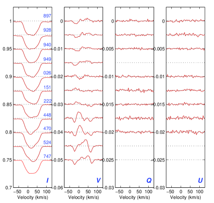
Figure 1: LSD mean Stokes $IVQU$ profiles. Rotational phases (according to the ephemeris given in Eq. (2) and multiplied by 1000) are given in the left panel. Apart from a marginal detection at phase 0.897, Stokes $Q$ and $U$ profiles are consistent with zero linear polarisation across the mean line. Variability of the Stokes $I$ profile is observed, and modulation of the Stokes $V$ profile shape by an apparently non-uniform Fe surface abundance distribution (analogous to that encountered for $\theta$ Aur by Wade et al. 2000a, for example) supports the view that variability of the mean Fe line results primarily from non-uniform surface abundances (see Sect. 6).

Circular polarisation (Stokes $V$) and linear polarisation (Stokes $Q$ and $U$) spectra of 36 Lyn were obtained during Feb/Mar 2000 and Dec 2001 using the MuSiCoS spectropolarimeter mounted on the 2 metre Bernard Lyot telescope at Pic du Midi observatory. The spectrograph and polarimeter module are described in detail by Baudrand & Böhm (1992) and by Donati et al. (1999) respectively. The standard instrumental configuration allows for the acquisition of circular or linear polarisation spectra with a resolving power of about 35,000 throughout the range 4500-6600 Å.

A complete Stokes $V$ circular polarisation observation consists of a series of 4 subexposures between which the polarimeter quarter-wave plate is rotated back and forth between position angles of $-45\degr$ and $+45\degr$. This procedure results in exchanging the orthogonally polarised beams throughout the entire instrument, with the aim of reducing systematic errors in polarisation measurements of sharp-lined stars to below a level of about 0.01% (Wade et al. 2000a). The procedure for recording Stokes $Q$ and $U$ linear polarisation observations is similar, except that the entire instrument is rotated (rather than the quarter-wave plate, which is removed from the beam for linear polarisation observations). Further details about the observing procedure are provided by Wade et al. (2000a).

In total 11 Stokes $V$, 8 Stokes $Q$ and 8 Stokes $U$ spectra of 36 Lyn were obtained, with peak signal-to-noise ratios (S/N) of typically 300:1 per pixel in Stokes $V$ and 325:1 in Stokes $Q$/$U$. In addition, during each run observations of various magnetic and non-magnetic standard stars were obtained within the context of other observing programmes (e.g. Shorlin et al. 2002, Kochukhov et al. 2004) which serve to verify the nominal operation of the instrument.

The log of spectropolarimetric observations of 36 Lyn is shown in Table 2.

2.3 IUE spectra

The IUE spectra employed in this study were the NEWSIPS-extracted, large aperture high-dispersion files from the Short Wavelength Prime (SWP) camera. These were downloaded from the MAST data archive. The data used were all 24 IUE SWP/large-aperture spectra for 36 Lyn, obtained during 3 epochs in 1985, 1987 and 1988. The data are described in more detail by Smith & Groote (2001).

2.4 Balmer-line Zeeman analyser polarimetric observations

Three measurements of the longitudinal magnetic field of 36 Lyn were obtained in 1992 using the University of Western Ontario (UWO) photoelectric polarimeter mounted on the 1.2 m telescope at the UWO Elginfield observatory. The polarimeter was employed as a Balmer-line Zeeman analyser to measure the fractional circular polarisation in the wings of H$\beta$ at $\pm 5.0$ Å from line centre. The longitudinal magnetic field was inferred from measured fractional circularly polarised flux using a conversion factor of 17500 G/%, as determined from scans of the H$\beta$ profile of 36 Lyn. The instrument and observing technique are described in detail by Landstreet (1982). The measurements are reported in Table 3.

3 Least-Squares Deconvolution and longitudinal magnetic field

We begin by applying the Least-Squares Deconvolution (LSD) multiline analysis procedure (Donati et al. 1997) to each of the MuSiCoS polarised spectra in order to obtain mean Stokes $IQUV$ profile sets (e.g. Wade et al. 2000a). LSD mean profiles were extracted using line masks derived from VALD line lists, corresponding to $T_{\rm eff}=13500$ K, $\log g=4.0$ (see Sect. 5), a minimum line depth of 10% and an abundance table specific to 36 Lyn (using abundances derived in Sect. 6). More information about the extraction of LSD profiles and the construction of LSD line masks is provided by Wade et al. (2000b) and Shorlin et al. (2002).

The LSD profiles (extracted for lines of Fe) are shown in Fig. 1. The Stokes $V$ profiles show complex structure, are clearly detected at all phases, and are strongly modulated as the star rotates. Remarkably, Stokes $Q$ and $U$ are never confidently detected, notwithstanding a typical LSD noise level below 0.015%. The Stokes $I$ profiles also show variability, which we interpret as rotational modulation of a non-uniform surface abundance distribution of Fe. This will be discussed in further detail in Sect. 7.

The longitudinal magnetic field $\langle B_{z}\rangle$ and its formal uncertainty $\sigma_{B}$ were inferred from each of the extracted LSD Stokes $I/V$ profile sets by numerical integration over velocity, in the manner described by Wade et al. (2000b).

The 11 new LSD longitudinal field measurements have typical uncertainties $\sigma_{B}\sim 60$ G, and range from -790 G to +876 G. The inferred values of the longitudinal field of 36 Lyn are reported in Table 3.

HJD	Phase	$\langle B_{z}\rangle$
($-$2450000)		(G)
2448739.621	0.622	$-90\pm 200$
2448744.609	0.922	$-790\pm 320$
2448754.676	0.548	$660\pm 260$
2451578.555	0.940	$-612\pm 48$
2451584.425	0.470	$595\pm 66$
2451586.556	0.026	$-91\pm 109$
2451596.520	0.624	$24\pm 56$
2451597.766	0.949	$-762\pm 52$
2451601.519	0.928	$-694\pm 68$
2451603.512	0.448	$662\pm 82$
2451606.479	0.222	$876\pm 68$
2451608.496	0.747	$-673\pm 50$
2452245.637	0.897	$-790\pm 90$
2452246.611	0.151	$609\pm 87$

Table 3: New longitudinal magnetic field measurements of 36 Lyn obtained from Balmer-line photopolarimetry (HJD 2448739-2448754) and from MuSiCoS LSD mean Stokes $I$ and $V$ profiles (HJD 2451578-). Phases are calculated according to the rotational ephemeris, Eq. (1), determined in Sect. 4. All uncertainties are $1\sigma$.

We have combined the 14 new measurements of the longitudinal magnetic field with 24 previously published measurements (2 reported by Borra, Landstreet & Thompson (1983) and 22 reported by Shore et al. (1990), all obtained using a Balmer line Zeeman analyser at H$\beta$) in order to determine the magnetic period. The periodogram of the longitudinal field data, obtained using a modifed Lomb-Scargle technique, is characterised by a strong, unique peak at $3.83495\pm 0.00003$ days (resulting in a reduced $\chi^{2}$ of 2.07 for a first-order harmonic fit, and where the formal $1\sigma$ error bar is derived using the reduced $\chi^{2}$ statistical tables of Bevington 1969). This period is consistent with, although more precise than, published magnetic and photometric values of the period (e.g. Shore et al. 1990, confirmed by Adelman (2000), $P_{\rm rot}=3.8345\pm 0.001$ days). This period has been kindly confirmed using minimum-false alarm probability methods by P. Reegen, who finds a best-fit period of 3.83495 days with a significance $\log S=3.34$.

It should be noted that a second-order fit to the magnetic data provides a significantly lower reduced $\chi^{2}$ (1.31). Independent fitting of the individual datasets (the Balmer-line measurements and the LSD metallic-line measurements) demonstrates that the Balmer-line data are well-described by a first-order fit, and that the second-order contribution comes entirely from the LSD data. The shapes of the longitudinal field variation as defined by the two datasets are therefore quite clearly different. This is not too surprising - it is well documented that longitudinal field variations derived from metallic-line measurements often contain non-sinusoidal contributions (e.g. Wade et al. 2000b), likely due to the presence of non-uniform distributions of these elements across the stellar surface.

4 Variations of the H$\alpha$ profile

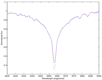
Figure 2: Variation of the H$\alpha$ profile core of 36 Lyn due to the magnetically-confined circumstellar disk (see Sect. 4 and 7).

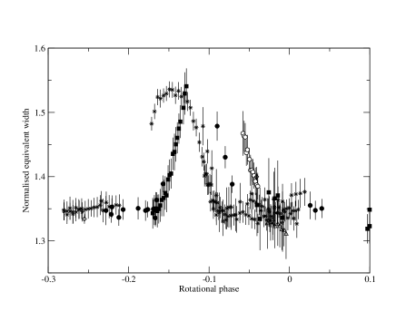
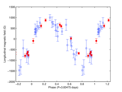
Figure 3: Upper frame - Variation of the H$\alpha$ profile core equivalent width and longitudinal field of 36 Lyn. Detail of primary occultation, measurements from all spectra, phased according to the adopted magnetic rotational period of 3.83495 days. Note the clear and systematic offset of measurements obtained at different epochs (represented by different symbols). Lower frame - Longitudinal magnetic field measurements phased according to the equivalent width period 3.83475 days. Note the apparent offset between the older (H$\beta$, open squares) and more recent (MuSiCoS, filled circles) longitudinal field measurements.

Upon examination of the optical spectra, it was immediately noted that the core depth of the H$\alpha$ line of 36 Lyn is strongly variable. Variability was first reported by Takada-Hidai & Aikman (1989), who attributed it to occultation of the stellar disc by the magnetically-confined circumstellar plasma. These authors obtained several observations of H$\alpha$, and noted that the core occasionally weakens, possibly accompanied by a depression of the inner wings. We confirm the variability, which is clearly intrinsic to H$\alpha$, and not (for example) the result of blending with strongly-variable metallic lines (the metallic-line variability of 36 Lyn is too weak, and no suitably-located lines exist in any case) or due to continuum registration errors (the continuum near H$\alpha$ in our spectra is uniformly excellent, and shows internal and external agreement amongst the datasets to within about 1%). However, in contrast to the observations of Takada-Hidai & Aikman, we observe no variability of the inner wings, and we observe a core which occasionally strengthens.

We have measured equivalent widths of the core of H$\alpha$ in all of our spectra, in the range 6561.0 to 6565.5 Å, after local reregistering of the spectra to further reduce systematic differences in continuum normalisation. Uncertainties associated with the equivalent widths were also calculated by adopting the inverse continuum signal-to-noise ratio as an approximate standard error bar associated with each spectrum pixel, and propagating these errors through the equivalent width calculation. We find that the measured H$\alpha$ equivalent width varies rather rapidly as a function of phase, with significant variations of about 15% (see Fig. 2).

When the H$\alpha$ equivalent width measurements are folded according to the magnetic period determined in Sect. 3, the various epochs are found to be offset in phase relative to one another by up to 0.06 cycles, as shown in Fig. 3 (upper frame). If we interpret these offsets to be the result of an error in the period determined from the magnetic measurements, they imply a best-fit equivalent width period (determined using Phase Dispersion Minimisation; Stellingwerf 1978) of $3.83475\pm 0.00002$ days. When phased according to this period, the equivalent width data show a clear, coherent variation, with a sharp maximum near phase 0.3, as well as a much weaker increase about one-half cycle later (Fig. 4). We interpret these variations in the context described by Shore, Brown & Sonneborn (1987). In this context, the increase in H$\alpha$ absorption results from occultation of the stellar disc by plasma which is confined magnetically near the magnetic equator, and forced to co-rotate with the star. The (neutral) H gas is coupled to the ionised gas as a result of frequent reionisations, as well as by collisions. This interpretation is supported by the presence of two peaks, separated in phase by approximately 0.5 cycles, and approximately coincident with magnetic crossover phases (when $\langle B_{z}\rangle\sim 0$). It is further supported by observed systematic changes in the radial velocity (RV) of the H$\alpha$ core coincident with the occultation phases. As would be expected, the core RV is initially blueshifted (with respect to the systemic RV) at the beginning of the occultation, and becomes redshifted as the occultation ends (this is illustrated in Fig. 5).

The intensities of the two occultation peaks are clearly unequal. This implies that the column depth of neutral H occulting the disc differs substantially at phases 0.0/0.5, i.e. that the occulting material is not distributed uniformly within or near the magnetic equatorial plane. The accumulation of gas overdensity at the intersections of the magnetic and rotational equators (i.e. at the nodal points) of magnetic Bp stars, and differences in the column density of these “clouds”, has been documented for the He-strong star $\sigma$ Ori E (e.g. Landstreet & Borra 1979), for example.

The physical conditions, structure and dynamics of the magnetically-confined wind will be discussed in more detail in Paper II.

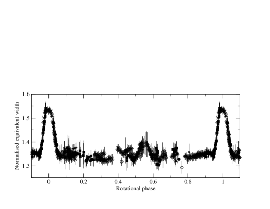
Figure 4: Variation of the H$\alpha$ profile core equivalent width of 36 Lyn, with measurements phased according to the equivalent width period 3.83475 d. Note the significant difference in amplitude of the $\phi\simeq 0.0$ and $\phi\simeq 0.5$ peaks. Error bars shown correspond to $2\sigma$ confidence.

The period deduced from the H$\alpha$ equivalent width data is not formally consistent with that determined using the magnetic data. However, when the magnetic data are phased according to the H$\alpha$ period, an acceptable phase variation is achieved. Although the new magnetic data show a small apparent offset in phase with respect to the archival data (Fig. 3, lower frame), this offset could easily result from well-known systematic differences in the shapes of field variations diagnosed from metallic vs. Balmer lines.

We therefore adopt the H$\alpha$ period as the rotational period of 36 Lyn. Hereinafter, all data have been phased according to the ephemeris:

$${\rm JD}=(2443000.451\pm 0.03)+(3.83475\pm 0.00002)\cdot{\rm E},$$ (1)

where the zero-point corresponds to the epoch of maximum H$\alpha$ core absorption.

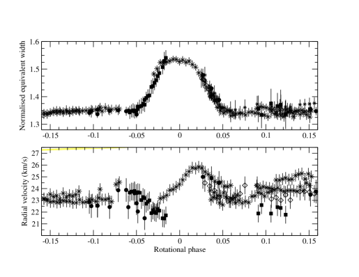
Figure 5: Variation of the equivalent width and radial velocity of the H$\alpha$ profile core of 36 Lyn during the primary occultation at phase 0.0. Measurements have been phased according to the equivalent width period 3.83475 d. Error bars shown correspond to $2\sigma$ confidence.

5 Fundamental characteristics of 36 Lyn

5.1 Fundamental parameters and evolutionary status

We begin by redetermining the effective temperature and surface gravity of 36 Lyn using published Geneva and $uvby\beta$ photometry, the observed spectral energy distributions at optical and UV wavelengths, and the H$\alpha$ and H$\beta$ profiles in our spectroscopic data.

Geneva photometry (from the Geneva photometric database, http://obswww.unige.ch/gcpd/ph13.html, Burki 2002) coupled with the calibration of North & Nicolet (1990) give $T_{\rm eff}=13650$ K and $\log g=3.75$. Strömgren photometry (Hauck & Mermilliod 1998) coupled with the calibration of Moon & Dworetsky (1985) give $T_{\rm eff}=13740$ and $\log g=3.65$.

Using theoretical flux spectra, we have fit the observed optical (Adelman & Pyper 1983) and UV (Jamar et al. 1976) spectrophotometry of 36 Lyn. Using a modified version of the ATLAS9 model atmosphere code (Kurucz 1993) and our photospheric abundance determinations (Sect. 6), we have performed this calculation for a grid of temperatures and gravities bracketing the photometric values, and various metallicities ranging from $1-10\times$ solar. We have offset magnetic broadening in the atmosphere model by assuming a 2 km s^-1 microturbulence. In Fig. 6 we show the observed energy distribution along with selected models. The best model fit to the energy distribution of 36 Lyn ($T_{\rm eff}=13300$ K, $\log g=4.0$, [M]=0.5) is shown in Fig. 6 (upper panel), as well as fits for ($T_{\rm eff}=13600$ K, $\log g=3.7$, [M]=0.0) and ($T_{\rm eff}=13000$ K, $\log g=4.0$, [M]=1.0). For the UV fluxes, we used TD1 data which was converted from flux into monochromatic magnitudes. We then reduced to 5000 Å using $m$(5000 Å)=5.37 (a value very close to the known $m_{V}$=5.32).

Finally, using ATLAS9 model Balmer line profiles for solar and enhanced metallicities, we have fit the observed wings of the H$\alpha$ and H$\beta$ profiles and obtain a best-fit for $T_{\rm eff}=13600$ K and $\log g=3.7$ (Fig. 6, lower frames).

All three models provide a satisfactory fit to the observed flux distribution in the optical region, while they differ in the UV region. As $E(B-V)=0.003$ for 36 Lyn (see, for example, Lucke L78 (1978)), this cannot be explained as due to unaccounted-for reddening. The model with the highest metallicity, 13000g40p10k2, provides the better fit below $\lambda$=1800 Å  (1/$\lambda$(microns)=5.5), while the moderate metallicity model, 13300g40p05k2, fits better in all spectral regions longer than 1800 Å. The higher temperature model does not fit the UV flux distribution, but it provides the best fit to the observed hydrogen line profiles. These systematic and significant discrepancies probably show true limitations of ATLAS9 model atmospheres in describing the photospheric structure of 36 Lyn.

As a compromise, we have adopted $T_{\rm eff}=13300\pm 300$ K for 36 Lyn, and have chosen a model with $T_{\rm eff}$=13300 K, $\log g$=4.0, and a logarithmic metallicity with respect to the sun of 0.5 for our abundance analysis. These values have been selected giving approximately equal weight to the energy distribution and Balmer lines, although we point out that they are rather arbitrary - it is really impossible to confidently select any model within the range $13000\leq T_{\rm eff}\leq 13600$ K, $3.7\leq\log g\leq 4.0$ or $0.0\leq$[M]$\leq 1.0$.

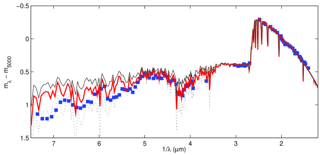
Figure 6: A comparison between the observed flux distribution in 36 Lyn (filled squares) and the theoretical distributions calculated with three selected atmospheric models: 13000g40p10k2 (dotted line), 13300g40p05k2 (thick line, and the adopted model), and 13600g37p00k2 (thin line). A comparison between the observed H$\beta$ (left panel) and H$\alpha$ (right panel) line profiles and synthesized with 13300g40p05k2 (full thick line) and 13600g37p00k2 (dotted line) models.

Now, using the derived temperature, along with the apparent visual magnitude ($m_{V}=5.3$), absolute magnitude ($M_{v}=-0.8$) and Hipparcos distance ($d=162\pm 15$ pc) reported by Gomez et al. (1998), we obtain the bolometric magnitude of 36 Lyn $M_{\rm bol}=-1.65\pm 0.4$ (using a bolometric correction $BC=-0.85$ determined using the interpolation formula of Balona 1994). The luminosity is therefore $\log L/L_{\odot}=2.54\pm 0.16$, and the stellar radius $R=3.4\pm 0.7\leavevmode\nobreak\ R_{\odot}$. From the $\log T-\log L/L_{\odot}$ HR diagram position of 36 Lyn (illustrated in Fig. 7), we obtain the stellar mass $M=4.0\pm 0.2M_{\odot}$ and age $\log t=8.0$ ($t=79-110$ Myr) based on the model evolutionary calculations for solar metallicity of Schaller et al. (1992). The combination of $R$ and $M$ give a logarithmic surface gravity of $\log g=4.0\pm 0.2$. We point out, as elaborated by Bagnulo et al. (2005), that the use of a bolometric corrections derived for normal stars, coupled with comparisons with solar metallicity evolutionary tracks, and uncertainties regarding the application of the Lutz-Kelker correction, likely underestimates the luminosity and age uncertainties.

The measured projected rotational velocity $v\sin i=48\pm 3$ km s^-1, obtained using individual metallic line profiles (see Sect. 6), and rotational period of $3.83475\pm 0.00002$ days imply a projected radius (assuming rigid rotation) of $R=(3.64\pm 0.23)\sin i\ R_{\odot}$. The radius determined from the HR diagram is numerically smaller than the projected radius determined from rigid rotation (although they are consistent within the uncertainties). The combination of the two radius estimates implies $i\geq 56\degr$, with a best-fit value of $i=90\degr$, and a true rotational speed in the range 45-61.5 km s^-1.

The derived fundamental and rotational characteristics of 36 Lyn are summarised in Table 4.

Mass (${\cal M}_{\odot}$)	$4.0\pm 0.2$
Radius (${\cal R}_{\odot}$)	$3.4\pm 0.7$
Age (y)	$0.79-1.1\times 10^{8}$
$T_{\rm eff}$ (K)	$13300\pm 300$
$\log g$	$3.7-4.2$
$v\sin i$	$48\pm 3$
Period	$3.83475\pm 0.00002$ d
$\sin i$	0.83-1.00

Table 4: Fundamental characteristics derived for 36 Lyn

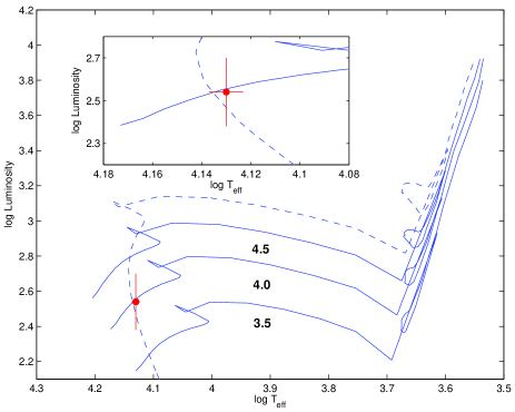
Figure 7: HR diagram position of 36 Lyn. The filled circle represents the derived position of 36 Lyn, solid curves are evolutionary tracks for 3.5, 4.0 and 4.5 $M_{\odot}$ for solar metallicity (Schaller et al. 1992), and the dashed curve is the associated isochrone for $10^{8}$ y.

5.2 Binarity

There is no indication of binarity in the literature, and the Hipparcos mission classifies 36 Lyn as single. The Stokes $I$ LSD profiles are constant in mean radial velocity at $+22\pm 2$ km s^-1. The H$\alpha$ profiles, outside of occultation phases, give $+23\pm 1$ km s^-1. Stickland & Weatherby (1984) find $v_{\rm rad}=+26\pm 1$ km s^-1, whereas the Bright Star Catalogue (Hoffleit et al. 1995) gives +21 km s^-1, Aikman (1976) gives $+21.9$ km s^-1, Abt (1970) gives $+26.4$, and Takada-Hidai & Aikman (1989; measured from H$\alpha$) give $+29.7\pm 1.6$ km s^-1. Although there exists some diversity among these measurements, this is expected given the metallic-line RV variations (due to surface features - see Sect. 6.3) and the H$\alpha$ RV variations (due to the circumstellar gas - see Sect. 4 and Paper II). Therefore we find no strong evidence for binarity.

5.3 Radio and X-ray emission properties

36 Lyn was observed at 6 cm using the VLA by Linsky et al. (1992), who found an upper limit ($3\sigma$) of $0.62$ mJy. More recently, it has been detected (at phase 0.73 according to our ephemeris) with a flux of $0.45\pm 0.05$ mJy at 3.6 cm (S. Drake, private communication).

Berghofer et al. (1996) found that ROSAT obtained no detection of X-rays at the position of 36 Lyn, reporting $\log L_{x}<29.84$.

5.4 Magnetic field geometry

5.4.1 Longitudinal field variation

For a tilted, centred dipole of polar strength $B_{\rm p}$, the variation of the longitudinal magnetic field $\langle B_{z}\rangle$ with rotational phase $\phi$ is given by Preston’s (1967) well-known relation

$$\langle B_{z}\rangle=B_{\rm p}{{15+u}\over{20(3-u)}}(\cos\beta\cos i+\sin\beta\sin i\cos 2\pi(\phi-\phi_{0})),$$ (2)

where $u$ denotes the limb darkening parameter and $\phi_{0}$ the phase of longitudinal field maximum (equal to $u=0.4$ and approximately $\phi_{0}=0.25$ in the particular case of 36 Lyn). The inclination and obliquity angles $i$ and $\beta$ are related by

$$\tan\beta={{1-r}\over{1+r}}\cot i,$$ (3)

where $r=-0.83\pm 0.1$ is the ratio of the longitudinal field extrema according to the best-fit sine curve.

From $r\simeq-1.0$ we obtain straightforwardly that either $i$ or $\beta$ is close to 90$\degr$, a result consistent with the rigid rotation model developed considering the stellar radius, period and $v\sin i$.

For our best-fit inclination $i=90\degr$, $\beta$ cannot be determined from Eq. (3) and Eq. (2) reduces to

$$\langle B_{z}\rangle^{max}=B_{\rm p}{{15+u}\over{20(3-u)}}\sin\beta.$$ (4)

In other words, the magnetic obliquity $\beta$ and polar strength of the dipole $B_{p}$ cannot be disentangled when $i=90\degr$, and we can only determine their product $B_{\rm p}\sin\beta=3380\pm 170$ G.

In the case of our minimum acceptable inclination $i=56\degr$, we obtain using Eq. (3) that $\beta=82\pm 5\degr$, and Eq. (2) gives $B_{p}=3760\pm 170$ G. Therefore, considering the full range of inclinations $56\degr-90\degr$ admitted by the data, we infer from the longitudinal field variation that $3210\leq B_{\rm p}\leq 3930$ G.

5.4.2 Stokes $V$ profiles

Using the method described by Donati et al. (2001) and Wade et al. (2005), we have compared the phase variation of the Stokes $V$ profiles with the Zeeman2 (Landstreet 1988, Wade et al. 2001) predictions of a grid of 9000 different magnetic field models, obtained by systematically varying $i$, $B_{d}$ and $\beta$ in the range 56-90$\degr$, 0 to -4000 G, and 0 to $180\degr$, respectively. For each model, the reduced $\chi^{2}$ of the observed and calculated Stokes $V$ profiles was calculated.

The best-fit solutions for the dipolar strength $B_{\rm d}$ and the magnetic obliquity $\beta$, for all admissible inclinations, are $B_{\rm d}=-1300$ G and $\beta=100$. Although both methods recover effectively the same value of the obliquity ($\beta=80\degr$ and $\beta=100\degr$ produce identical longitudinal field variations), the dipole strength obtained from the profile fits is abour 3 times smaller than that determined from the longitudinal field.

We strongly suspect that these (significant) differences result from the important modulation of the Stokes $V$ profiles by the non-uniform distribution of Fe on the stellar surface. In fact, the best-fit model for Stokes $V$, while reproducing the amplitudes of the weak signatures around phases 0.9-0.2 rather well, is totally unable to reproduce the stronger Stokes signatures at phases 0.5-0.8. This failure is reflected in the very high reduced $\chi^{2}$ statistic ($\chi^{2}/\nu\sim 10.4$) obtained for the Stokes $V$ profiles. Moreover, the structure and radial velocities of features apparent in the observed Stokes $V$ profiles (see Fig. 1) are not evident in the calculated profiles. This suggests that the model we have used to calculate the profiles of the LSD mean profiles is an obvious oversimplification of the true surface structure of 36 Lyn. Additional attempts to reproduce this structure using higher-order multipolar magnetic field models were unsuccessful. We therefore conclude that the structure of the Stokes $V$ profiles is likely due to a strongly nonuniform distribution of Fe on the surface of the star. This will be discussed further in Sect. 6.

Finally, we report that Stokes $Q$ and $U$ profile corresponding to the best-fit Stokes $V$ dipole model (with $|B_{\rm p}|=1300$ G) have amplitudes similar to the typical noise in the associated LSD profiles. For the dipole model derived from the longitudinal field data (with $|B_{\rm p}|=3380$ G), the predicted linear polarisation amplitudes are several times larger than the observed Stokes $Q$ and $U$ upper limits. This is consistent with results obtained for other magnetic Ap/Bp stars by Wade et al. (2000a), and may reflect the influence of non-uniform abundance distributions, or small-scale structure of the magnetic field, on the disc-integrated polarimetric signal.

6 Photospheric chemical abundances

6.1 Mean abundances

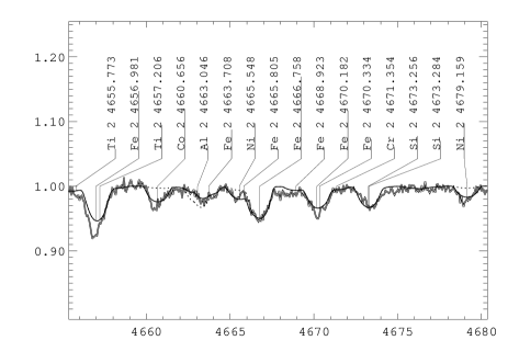
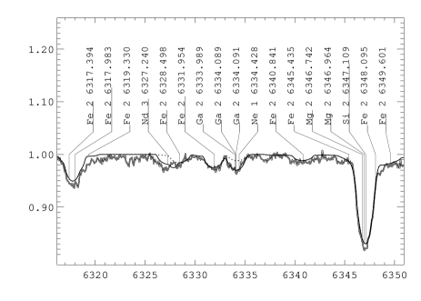
Figure 8: A comparison between the observed and synthesized spectra in the regions of Al ii, Co ii, and Ni ii  lines (left panel) and Si ii, Ga ii, and Nd iii  lines (right panel). Calculations with the Al, Co, Ni, Ga and Nd abundances derived from our analysis are shown by the full line, and those with the UV abundances (except Fe and Ti) are shown by the dotted line. The dotted line also represents the Nd iii  line with a 1.0 dex reduced abundance.

Mean (phase-averaged and surface-averaged) photospheric abundances were determined from analysis of both optical and UV spectra of 36 Lyn. Some previously published UV abundances were also obtained from the literature. All abundances are reported in Table 5.

6.1.1 Optical abundances

Synthetic spectrum calculations for the whole spectral region covered by the optical observations (4500-6600 Å) were performed with the synthetic spectrum codes synth (Piskunov 1992) and starsp (Tsymbal 1996). Selected regions of the spectrum were also modeled using Zeeman2 (Landstreet 1988, Wade et al. 2001). For hydrogen line profiles we used the more recent calculations of the hydrogen line opacities (Barklem at al. 2002). We did not include the magnetic field for synth or starsp synthetic calculations; instead, we employed a pseudomicroturbulence of 2 km s^-1  to account for magnetic intensification. The influence of a dipolar magnetic field of surface intensity 3 kG was employed for the Zeeman2 calculations. The adopted model atmosphere is an ATLAS9 model with the adopted parameters described in Sect. 5. We have explored the range of model parameters discussed in Sect. 5.1, derived from the photometry, energy distribution and Balmer lines, and we find that the detailed choice of model atmosphere has a negligible impact on the derived abundances. With a few exceptions, all atomic data were extracted from the VALD database (Kupka et al. 1999, Ryabchikova et al. 1999). Rare earth abundances (Pr and Nd) were derived from the lines of the second ionization stage with the transition probabilities from Cowley & Bord (1998), Bord (2000) - Nd iii, and from Bord (private communication) - Pr iii. Two lines of Ga ii, $\lambda\lambda$ 6334, 6419 were used for the gallium abundance determination in the optical region. Hyperfine and isotopic splitting (Karlsson & Litzén 2000) were taken into account.

In order to fit the line profiles, it was necessary to determine the projected rotational velocity $v\sin i$. Various estimates of $v\sin i$ exist in the literature, ranging from 40 km s^-1(Abt & Morrel 1995) to 60 km s^-1(Abt, Levato & Grosso 2002). We find $v\sin i=48\pm 3$ km s^-1, consistent with the recent results of Royer et al. (2002) who find $v\sin i=49$ km s^-1.

Fig. 8 shows a part of the 36 Lyn optical spectrum and synthetic spectrum fits.

	36 Lyn Optical1	36 Lyn UV	$\odot$
Element	$\log n/n_{\rm tot}$	$\log n/n_{\rm tot}$	$\log n/n_{\rm tot}$
He	$-1.65\pm 0.05$		-1.05
C	-3.0 - -2.7	-3.481	-3.48
O	-3.4 - -3.0		-3.11
Ne	-3.8 - -3.95		-3.95
Na	-5.30		-5.71
Mg	-4.35	$-4.44\pm 0.22^{2}$	-4.46
Al	-6.30	$-6.10\pm 0.15^{2}$	-5.57
Si	$-4.10\pm 0.2$	$-4.5:\pm 0.4^{1}$	-4.49
		$-4.70\pm 0.10^{2}$
P	-6.30		-6.59
S	-4.8 - -5.0		-4.83
Cl	-5.2		-6.54
Ti	$-5.00\pm 0.25$		-7.05
Cr	$-5.00\pm 0.3$	-5.31,	-6.37
		$-5.3\pm 0.4^{3}$
Mn	-5.8	$-6.80\pm 0.15^{3}$	-6.65
Fe	$-3.45\pm 0.25$	-3.21	-4.37
		$-3.90\pm 0.1^{3}$
Co	$-5.00\pm 0.15$	$-6.2\pm 0.2^{3}$	-7.12
Ni	$-4.90\pm 0.15$	$-5.7\pm 0.1^{3}$	-5.79
Cu		$-8.1\pm 0.6^{4}$	-7.83
Ga	$-6.05\pm 0.1$	$-6.90\pm 0.55^{5}$	-9.16
Pr	$-8.1\pm 0.2$		-11.33
Nd	$-7.7\pm 0.2$		-10.54

Table 5: Mean photospheric chemical abundances of 36 Lyn. Also shown are the respective solar abundances. Sources: ¹This work, ²Smith (1993), ³Smith & Dworetsky (1993), ⁴Smith (1994), ⁵Smith (1996).

6.1.2 Ultraviolet abundances

Ultraviolet abundances were inferred from spectrum synthesis using the synspec code (Hubeny, Lanz & Jeffery 1994), assuming a Kurucz (1993) ATLAS9 model atmosphere.

Notably, we discovered that the silicon abundances derived from Si ii and Si iii lines differed, a problem that we ultimately traced to a series of blends in the Si iii lines and which may potentially lead to erroneous abundances of Si derived for Bp stars from IUE data (two good, unblended Si iii lines are those at 1370.0 Åãnd 1417.2 Å.) We were finally able to distinguish the unblended and blended Si iii lines by their variability, as the former show variations in their radial velocity with phase, as reported from an optical Si line study by Stateva (1997).

6.2 Mean abundances and evidence for vertical abundance non-uniformities

In our analysis of optical spectra of 36 Lyn, we find no systematic differences in the abundances required to fit strong versus weak lines of elements with sufficiently rich line spectra. This suggests that stratification of these elements in the atmosphere of 36 Lyn is either very weak or nonexistent.

For a few elements, the abundances obtained from optical lines differ from those derived from UV lines. These differences cannot be explained by small differences in the adopted atmospheric parameters. The largest disagreements occur for Mn, Co, Ni and Ga which appear to be less abundant from the UV analysis, while Al is opposite. The Ga problem is well known (Lanz et al. 1993). Dworetsky & Smith (1993) derived abundances from the low excitation UV Mn ii, Co ii  and Ni ii  lines, while our analysis is based on high excitation lines. Therefore a difference in the UV and optical abundances may reflect stratification of these elements, although the discrepancy could be attributed to unidentified blends given the relative scarcity of lines of these elements in the optical. An examination of the oscillator strengths used in the various studies indicates that systematic errors in $gf$ values cannot explain the differences. For Co ii lines, neglect of hyperfine structure may be an important contributor.

Overall, we find that He is depleted relative to solar, while Fe peak elements are strongly enhanced, by one dex or more. Abundances of two rare earth elements (REEs, Pr and Nd) are found to be enhanced by approximately 3 dex. Mn, Co, Ni and Ga may be stratified.

6.3 Horizontal abundance non-uniformities

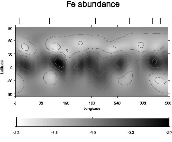
Figure 9: Fe Doppler image from Fe ii $\lambda$4522. Right frame - comparison of observed and calculated profiles. Left frame - Derived abundance map in rectangular projection. Tick marks indicate phases of 36 Lyn observations used to derive the map.

The variations of lines of a number of elements in the high-resolution optical spectrum of 36 Lyn as well as the LSD profiles are suggestive of non-uniform horizontal distributions of their abundances. However, some care is required in interpreting these variations: Smith & Groote (2001) caution that the magnetically-confined winds of Bp stars can produce optical line profile variability due to occultation of the stellar disc by the circumstellar material, and that in a number of hot Bp stars a significant component of the optical metallic-line variability can be attributed to this phenomenon.

In the spectrum of 36 Lyn, weak variability occurs in lines of He, Fe, Si, Cr, Ti, and Mg (based on our own spectra, as well as the results of Stateva 1997). Some of these elements show extrema of their equivalent width phase variations which coincide with the magnetic extrema (phases 0.25/0.75, either in phase or anti-phase, e.g. He, Fe) whereas others show variations with extrema at crossover phases (phases 0.0/0.5, e.g. Si). We have also examined the dependence of EW variation shape and phase of Fe lines as a function of excitation potential, and find no significant dependence. Based on (1) the variety of equivalent width variability characteristics, (2) the large range in excitation potential of lines that undergo variability, (3) the modulation of the shapes of Stokes $V$ profiles and (4) the apparent difference in the extrema of the longitudinal field variations as diagnosed in metal versus H lines, we conclude that the optical line profile variations result substantially from surface structure (magnetic + abundance non-uniformity), rather than being due to the circumstellar material. This conclusion is supported by an examination of the high-resolution line profiles. As can be seen in Figs. 1 and 9, Fe lines exhibit variations in Stokes $I$ and $V$ profile shapes, consistent with Doppler modulation by surface non-uniformities.

Stateva (1997) attempted an harmonic reconstruction of the surface distributions of He, Si, Cr and Mg using equivalent width variations extracted from photographic spectra of 36 Lyn, and assuming that the variations were due entirely to surface non-uniformities. She was able to reproduce the (relatively low signal-to-noise ratio) equivalent width and radial velocity variations, and the resulting maps suggest that He, Si and Cr are concentrated primarily in the plane of the magnetic equator.

Here, we apply the more stringent test of attempting to reproduce the detailed line profile variations using the Doppler Imaging technique, for the particular case of Fe. Because we have only 11 high-resolution spectra, we are not attempting to derive a definitive map of the surface Fe distribution. Our primary goal is rather to demonstrate that the detailed profile variations of moderate and high-excitation Fe lines in the optical can be substantially explained by an inhomogeneous surface distribution of this element, and are not significantly affected by absorption due to the circumstellar material.

Doppler imaging is a technique which allows the inversion of observed spectral line profile variations to produce a two-dimensional map of the abundance distribution at the surface of a star. An inhomogeneity on the stellar surface leads to distortions in the spectral line profiles. These distortions appear on the blue side of the line profile as the spot comes into sight on the visible hemisphere of the star, travel across the spectral line and disappear on the red wing as the spot rotates out of sight. The longitudinal position of the inhomogeneity is obtained directly from the velocity position of the distortion within the profile, whereas its latitude has to be deduced from spectral time series. In INVERS12, the Doppler Imaging code we applied, developed by N. Piskunov and refined by O. Kochukhov (Kochukhov et al. 2004b), the equation of radiative transfer is solved in a way that allows the calculation of maps of several chemical elements simultaneously and self-consistently. In this program the precalculated local line profile tables used in former versions of the code are replaced by the calculation of specific intensities for each visible surface element on each iteration.

For 36 Lyn, we assumed various inclination angles between $56\degr$ and $90\degr$ to perform the Doppler Imaging. The best fit to the profiles was found for $i=60\degr$, although the dependence of the fit quality on $i$ was rather weak (and in particular this dependence cannot be used to constrain the inclination). We derived the Fe abundance on the surface of the star using several Fe ii lines, including $\lambda 4520,\lambda 4522,\lambda 5018,\lambda 5534$ and $\lambda 5780$, each of which produced a similar Fe distribution. In Fig. 9 we show the Fe distribution, in the rotational frame of reference, reconstructed from Fe ii $\lambda$4522.6 ($\chi_{e}=2.8$ eV). The distribution is characterised by a very patchy ring-like structure between -30°and +30° in stellar latitude, with a total contrast of somewhat more than 3 dex. Due to the uncertainty in the magnetic field geometry, it is difficult to conclude whether any obvious geometrical relationship exists between the Fe surface distribution and the magnetic field. Our success in interpreting the profile variations of the Fe ii lines supports our interpretation of the Fe (and other metal) line variations are due to Doppler modulation of surface structure. The details of the derived map should be interpreted conservatively, given that the map was derived using a single line with relatively coarse rotational phase coverage.

7 Discussion and conclusion

We have performed a thorough reevaluation and analysis of the physical and spectroscopic characteristics of the B8p He-weak star 36 Lyncis. Based on measurements of the longitudinal magnetic field, as well as measurements of the core equivalent width of the H$\alpha$ line, we have redetermined the rotational period $P_{\rm rot}=3.83475\pm 0.00003$ days. An examination of the variability of the H$\alpha$ core equivalent width reveals strong changes coincident with magnetic crossover phases, which we interpret as due to occultation of the stellar disc by magnetically-confined circumstellar gas. We have determined the effective temperature, radius, mass, age, projected and true rotational velocities, the rotation axis inclination, and we have summarised evidence for binarity, radio and X-ray emission.

We have found systematic and significant discrepancies between the temperature and gravity determined from the optical and UV energy distribution and from the Balmer lines, concluding that they probably show true limitations of the ATLAS9 model atmospheres in describing the real photospheric structure of 36 Lyn. The ATLAS9 models we have employed are calculated using scaled solar metallicities, while individual abundances in the atmosphere of 36 Lyn show large diversity. To check the influence of anomalous abundances on the model atmosphere structure, a few model atmospheres were calculated with LLmodels model atmosphere code (Shulyak et al. LL04 (2004)) which takes into account the contribution of individual line opacities to the total continuum opacity through direct synthetic calculations. This code allows us to examine the influence of the particular abundance table of 36 Lyn on the model atmosphere structure. The flux distribution for an LLmodels model with $T_{\rm eff}$=13300, $\log g=4.0$ and the abundances of 36 Lyn actually provides a somewhat better simultaneous fit to both the energy distribution and Balmer lines. We conclude that a model atmosphere with individualised abundances improves the overall fit to the observables, although discrepancies are still evident (a surface gravity below 4.0 is still required to fit the H lines). Possibly we are seeing the influence of peculiar and possibly stratified abundances on the photospheric temperature and pressure structure - effects which are not included in LLmodels.

We have modeled Least-Squares Deconvolved Stokes $V$ profiles and the longitudinal field variation to constrain the magnetic field geometry. We have analysed both optical and UV spectra and, using spectrum synthesis techniques, we have determined the abundances of 21 elements. We find no evidence for vertical stratification of most elements, although for a few elements (e.g. Mn, Co, Ni, Ga) we have derived abundances in the optical which differ from those in the UV, suggesting that these elements may be stratified. The influence of using an LLmodels individualised abundance model atmosphere on inferred abundances is small ($\pm$0.1 dex) for all elements except He, for which the abundance is decreased by 0.4 dex. On the other hand, using the individualised abundance model decreases by 0.15 dex the difference between the optical and UV Ga abundances (Ga optical abundance is decreased by 0.1 dex and Ga UV abundance increased by 0.05 dex).

We find convincing evidence exists for nonuniform surface (horizontal) distributions of some elements. Using the Doppler Imaging technique, we have constructed an approximate surface map of the Fe abundance distribution, which is characterised by a patchy ring-like structure between $-30\degr$ and $+30\degr$, and a contrast of somewhat more than 3 dex. The results reported in this paper set the stage for a detailed study of the structure and geometry of the circumstellar material in Paper II.

References

- (1) Abt H. & Levato H., 1978, PASP 90, 201
- (2) Abt H., Levato H. & Grosso M., 2002, ApJ 573, 539
- (3) Abt H.A. & Morrell N.I., 1995, ApJS 99, 135
- (4) Adelman S.J., 1984, MNRAS 206, 637
- (5) Adelman S.J., 2000, A&A 357, 548
- (6) Adelman S.J. & Pyper D., 1983, A&A 118, 313
- (7) Aikman G.C.L., 1976, PDAO 14, 379
- (8) Babel J., Montmerle T., 1997, A&A 323,121
- (9) Bagnulo S., Landstreet J.D., Mason E., Andretta V. et al., 2005, submitted to A&A
- (10) Balona L.A., 1994, MNRAS 268, 199
- (11) Barklem, P. S., Stempels, H. C., Allende Prieto, C., Kochukhov, O. P., Piskunov, N., O’Mara, B. J. 2002, A&A 385, 951
- (12) Baudrand J., Böhm T., 1992, A&A 259, 711
- (13) Berghoefer T.W., Schmitt J.H.M.M. & Cassinelli J.P., 1996, A&AS 118, 481
- (14) Bevington, P.R., 1969, Data reduction and error analysis for the physical sciences,McGraw-Hill, New York
- (15) Bolton C.T., 1994, Ap&SS 221, 95
- (16) Borra E.F. & Landstreet J.D., 1983, ApJS 53, 151
- (17) Bord D. 2000, A&AS 144, 517
- (18) Borra E.F., Landstreet J.D., Thompson I.B., 1983, ApJS 53, 151
- (19) Brown D.N., Shore S.N., Sonneborn G., 1985, AJ 90, 1354
- (20) Burki G., 2002, GENEVA photometric database
- (21) Chadid M., Wade G. A., Shorlin S. L. S., Landstreet, J. D., 2004, A&A 413,1087
- (22) Cowley A., 1972, AJ 77, 750
- (23) Cowley C.R., Bord D.J. 1998, in The Scientific Impact of the Gaddard High Resolution Spectrograph, C.C., eds, J.C. Brandt, T.B. Ake, C.C. Peterson (eds), ASP Conf. Ser. 143, 346
- (24) Donati J.-F., Wade G.A., Babel J., Henrichs H.F., de Jong J.A., 2001, MNRAS 326, 1265
- (25) Donati J.-F., Semel M., Carter B., Rees D.E., Cameron A.C., 1997, MNRAS 291, 658
- (26) Donati J.-F., Catala C., Wade G.A., Gallou G., Delaigue G., Rabou P., 1999, A&AS 134, 149
- (27) Drake Stephen A., Abbott David C., Bastian T. S., Bieging J. H., Churchwell E., Dulk G., Linsky Jeffrey L., 1987, ApJ, 322, 902
- (28) Drake S. A., Linsky J. L., Bookbinder J. A., 1994, AJ, 108, 2203
- (29) Drake S., 1998, Cont. Ast. Obs. Skalnaté Pleso, 3, 382
- (30) Drake S.A, Linsky J.L., Wade G.A., 2002, proceedings of the 201st meeting of the American Astronomical Society
- (31) Edwards D.L., MNRAS, 1932, 92, 389
- (32) Gomez A.E., Luri X., Gernier S., Figueras F., North P., Royer F., Torra J., Messessier M.O., 1998, A&A 336, 953
- (33) Hauck B. & Mermilliod M. 1998 A&AS, 129, 431
- (34) Hoffleit, E. D. & Warren W. H. Jr. 1995, Yale Bright Star Catalogue 5th revised edition (New Haven: Yale Univ. Obs.)
- (35) Jamar C., Macau-Hercot D., Monfils A., Thompson G.I., Houziaux L., Wilson R. 1976, ESA SR-27, 258
- (36) Karlsson N., Litzén U. 2000, J. Phys. B, 33, 2929
- (37) Kochukhov O., Bagnulo S., Wade G.A., Sangalli L., Piskunov N., Landstreet J.D., Petit P., Sigut T.A.A., A&A 414, 613
- (38) Kochukhov O., Drake N.A., Piskunov N., de la Reza N., 2004b, A&A 424, 935
- (39) Kupka F., Piskunov N., Ryabchikova T.A., Stempels H.C., Weiss W.W., 1999, A&AS 138, 119
- (40) Kurucz R.L., 1993, CD-ROM 13 (atlas9 atmospheric models) and 18 (atlas9 and synthe routine, line database)
- (41) Landstreet J.D. & Borra E.F., 1978, ApJ 224, L5
- (42) Landstreet J.D. & Borra E.F., 1979, …
- (43) Landstreet J.D., 1982, ApJ 258, 639
- (44) Landstreet J.D., 1988, ApJ 326, 967
- (45) Lanz, T., Artru, M.-C., Didelon, P. & Mathys G. 1993. A&A, 272, 465
- (46) Linsky J.L., Drake S.A., Bastian T.S., 1992, ApJ 393, 341
- (47) Lucke, P. B. 1978, A&A, 64, 367
- (48) Mihalas D. & Hearnshaw J.L., 1966, ApJ 144, 25
- (49) Molnar M.R., 1972, ApJ 175, 453
- (50) Moon T.T., Dworetsky M.M., 1985, MNRAS 217, 305
- (51) Nakajima, 1985, Ap&SS, 116, 285
- (52) Neiner C., Henrichs H. F., Floquet M., Frémat Y, et al., 2003, A&A 411, 565
- (53) North P. & Nicolet B., 1990, A&A 228, 78
- (54) Piskunov, N. 1992, Stellar Magnetism – Proceedings of the international meeting on the problem Physics and Evolution of Stars, ed. Yu. V. Glagolevskij & I.I. Romanyuk, St. Petersburg, p 92
- (55) Preston G.W., 1967, ApJ 150, 547
- (56) Preuss O., Schleussler M., Holzwarth V, Solanki S.K., 2004, A&A 417, 987
- (57) Royer F., Grenier S., Baylac M.-O., Gómez A. E., Zorec, J., A&A 393, 897
- (58) Ryabchikova T., Stateva I. 1996, in Model Atmospheres and Spectral Synthesis, ed. S.J. Adelman, F. Kupka & W.W. Weiss, ASP Conf. Ser., 108, 265
- (59) Ryabchikova, T. A., Piskunov, N., Stempels, H. C., Kupka, F., & Weiss, W. W. 1999, Phys. Scr., T83, 162
- (60) Sadakane K., 1984, PASP 96, 259
- (61) Sargent A.I., Greenstein J.L. & Sargent W.L.W., 1969, ApJ 157, 757
- (62) Searle L. & Sargent W.L.W., 1964, ApJ 139, 793
- (63) Shore S.N., 1987, AJ 94, 731
- (64) Shore S.N. & Brown D.N., 1990, ApJ 365, 665
- (65) Shore S.N., Brown D. & Sonneborn G., 1987, AJ 94, 737
- (66) Shore, Steven N.; Brown, Douglas N.; Sonneborn, George; Landstreet, John D.; Bohlender, David A., 1990, ApJ 348, 242
- (67) Shorlin S.L.S., Wade G.A., Donati J.-F., Landstreet J.D., Petit P., Sigut T.A.A., Strasser S., 2002, A&A 392, 637
- (68) Shulyak, D., Tsymbal, V., Ryabchikova, T., Stütz, Ch, & Weiss, W.W. 2004, A&A, 428, 993
- (69) Smith K.C., Dworetsky M.M. 1993, A&A 274, 335
- (70) Smith K.C., 1993, A&A 276, 393
- (71) Smith K.C., 1994, A&A 291, 521
- (72) Smith K.C., 1996, A&A 305, 902
- (73) Smith M. et al. 2006, in preparation (“Paper II”)
- (74) Smith M.A. & Groote D., 2001, A&A 372, 208
- (75) Stateva I.K., 1997, Ap&SS 250, 245
- (76) Stellingwerf R.F., 1978, ApJ 224, 953
- (77) Stickland D.J. & Weatherby J., 1984, A&AS 57, 55
- (78) Takada-Hidai M. & Aikman G.C.L., 1989, PASP 101, 699
- (79) Townsend R.H.D¿ & Owocki S.P., 2005, MNRAS 357, 251
- (80) Tsymbal, V.V. 1996, in Model Atmospheres and Spectral Synthesis, ed. S.J. Adelman, F. Kupka & W.W. Weiss, ASP Conf. Ser., 108, 198
- (81) ud-Doula A. & Owocki S, 2002, ApJ 576, 413
- (82) Wade, G.A., Donati, J.-F., Landstreet, J.D., Shorlin, S.L.S., 2000, MNRAS 313, 823
- (83) Wade, G.A., Donati, J.-F., Landstreet, J.D., Shorlin, S.L.S., 2000, MNRAS 313, 853
- (84) Wade G.A., Bagnulo S., Kochukhov O., Landstreet J.D., Piskunov N., Stift M., 2001, A&A,
- (85) Wade G.A., Fullerton A.W., Donati J.-F., Landstreet J.D., Petit P., Strasser S., 2005, in preparation