Stellar and gaseous velocity dispersions in type II AGNs at $0.3<z<0.83$ from the Sloan Digital Sky Survey

Abstract

We apply the stellar population synthesis code by Cid Fernandes et al. to model the stellar contribution for a sample of 209 type II AGNs at $0.3<z<0.83$ from the Sloan Digital Sky Survey. The reliable stellar velocity dispersions ($\sigma_{*}$) are obtained for 33 type II AGNs with significant stellar absorption features. According to the $L_{\rm[OIII]}$ criterion of $3\times 10^{8}\mbox{\,$\rm L_{\odot}$}$, 20 of which can be classified as type II quasars. We use the formula of Greene & Ho to obtain the corrected stellar velocity dispersions ($\sigma_{*}^{c}$). We also calculate the supermassive black holes masses from $\sigma_{*}^{c}$ in these high-redshift type II AGNs. The [O III] luminosity is correlated with the black hole mass (although no correlation between the extinction-corrected [O III] luminosity and the black hole mass), and no correlation is found between the Eddington ratio and the [O III] luminosity or the corrected [O III] luminosity. Three sets of two-component profile are used to fit multiple emission transitions ([O III]$\lambda\lambda$4959, 5007 and [O II]$\lambda\lambda$3727, 3729) in these 33 stellar-light subtracted spectra. We also measure the gas velocity dispersion ($\sigma_{g}$) from these multiple transitions, and find that the relation between $\sigma_{g}$ and $\sigma_{*}^{c}$ becomes much weaker at higher redshifts than in smaller redshifts. The distribution of $<\sigma_{g}/\sigma_{*}^{c}>$ is $1.24\pm 0.76$ for the core [O III] line and $1.20\pm 0.96$ for the [O II] line, which suggests that $\sigma_{g}$ of the core [O III] and [O II] lines can trace $\sigma_{*}^{c}$ within about 0.1 dex in the logarithm of $\sigma_{*}^{c}$. For the secondary driver, we find that the deviation of $\sigma_{g}$ from $\sigma_{*}^{c}$ is correlated with the Eddington ratio.

1 INTRODUCTION

Recent advances in the study of normal galaxies and active galactic nuclei (AGNs) are ample observational evidence for the existence of central supermassive black holes (SMBHs) and the relationship between SMBHs and bulge properties of host galaxies (Gebhardt et al. 2000; Ferrarese & Merritt 2000; Tremaine et al. 2002; Begelman 2003; Shen et al. 2005). We can use the stellar and/or gaseous dynamics to derive the SMBHs masses in nearby inactive galaxies. However, it is much more difficult for the case of AGNs. With the broad emission lines from broad-line regions (BLRs)(e.g. H$\beta$, Mg II, CIV; H$\alpha$), the reverberation mapping method and the empirical size-luminosity relation can be used to derive the virial SMBHs masses in AGNs (Kaspi et al. 2000; Vestergaard 2002; McLure & Jarvis 2002; Wu et al. 2004; Greene & Ho 2006a). It has been found that nearby galaxies and AGNs follow the same tight correlation between the central SMBHs masses ($M_{\rm BH}$) and stellar bulge velocity dispersion ($\sigma_{*}$) (the $M_{\rm BH}-\sigma_{*}$ relation) (Nelson et al. 2001; Tremaine et al. 2002; Greene & Ho 2006a, 2006b), which also implied that the mass from reverberation mapping method is reliable.

According to AGNs unification model (e.g. Antonucci 1993; Urry & Padovani 1995), AGNs can be classified into two classes depending on whether the central engine and BLRs are viewed directly (type I AGNs) or are obscured by circumnuclear medium (type II AGNs). In type I AGNs, by using the broad emission lines from BLRs (the reverberation mapping method or the empirical size-luminosity relation), we can derive virial SMBHs masses. It is not easy to study their host galaxies because their optical spectra are dominated by the non-stellar emission from the central AGNs activity. This is especially true for luminous AGNs, where the continuum radiation from central source outshines the stellar light from the host galaxy.

In type II AGNs, the obscuration of BLRs makes both the reverberation mapping method and the empirical size-luminosity relation infeasible to derive SMBHs masses. However, we can use the well-known $M_{\rm BH}-\sigma_{*}$ relation to derive SMBHs masses if we can accurately measure the stellar bulge velocity dispersion ($\sigma_{*}$). There are mainly two different techniques to measure $\sigma_{*}$, one is the ”Fourier-fitting” method (Sargent et al. 1977; Tonry & Davis 1979), the other is the ”Direct-fitting” method (Rix & White 1992; Greene & Ho 2006b and reference therein). These years it has been successful to derive $\sigma_{*}$ through fitting the observed stellar absorption features, such as Ca H+K $\lambda\lambda$ 3969, 3934, Mg Ib$\lambda\lambda$ 5167, 5173, 5184 triplet, and Ca II$\lambda\lambda$ 8498, 8542, 8662 triplet, etc, with the combination of different stellar template spectra broadened by a Gaussian kernel (e.g. Kauffmann et al. 2003; Cid Fernandes et al. 2004a; Greene & Ho 2006b).

On the other hand, Nelson & Whittle (1996) find that the gaseous velocity dispersion ($\sigma_{g}$) of [O III]$\lambda$5007 from the narrow-line regions (NLRs) is nearly the same as $\sigma_{*}$ for a sample of 66 Seyfert galaxies, and suggest that the gaseous kinematics of NLRs be primarily governed by the bulge gravitational potential. Nelson (2001) find a relation between $M_{\rm BH}$ and $\sigma_{\rm[OIII]}$ (the [O III]$\lambda$5007 velocity dispersion) for AGNs, very similar to the relation of $M_{\rm BH}-\sigma_{*}$, although with more scatter, which strongly suggests that $\sigma_{g}$ can be used as a proxy for $\sigma_{*}$. For lower-redshift type II AGNs with $0.02<z<0.3$, Kauffmann et al. (2003) have investigated the properties of their hosts from the Sloan Digital Sky Survey (SDSS) Data Release One (DR1), measured $\sigma_{*}$ and estimated the SMBHs masses from $\sigma_{*}$ (Brinchmann et al. 2004). By using this sample, Greene & Ho (2005) have measured the gaseous velocity dispersion ($\sigma_{\rm g}$) from multiple transitions ([O II] $\lambda$3727, [O III] $\lambda$5007, and [S II] $\lambda\lambda$6716, 6731) and compared $\sigma_{*}$ and $\sigma_{g}$. They find that $\sigma_{g}$ from these multiple transitions trace $\sigma_{*}$ very well, although some emission features they show considerable scatters.

Type II quasars are the luminous analogs of low-luminosity type II AGNs (such as Seyfert 2 galaxies). The obscuration of BLRs makes quasars appear to be type II quasars (obscured quasars). Some methods have been used to discover type II quasars, but only a handful have been found. Recently, Zakamsa et al. (2003) present a sample of 291 type II AGNs at redshifts $0.3<Z<0.83$ from the SDSS spectroscopic data. About half are type II quasars if we use the [O III] $\lambda$5007 line luminosity to represent the strength of the nuclear activity. What is the $\sigma_{*}-\sigma_{g}$ relation for type II quasars? And what are their SMBHs masses and the Eddington ratios $L_{\rm bol}/L_{\rm Edd}$ (i.e. the bolometric luminosity as a fraction of the Eddington luminosity)?

Here we use the sample of Zakamsa et al. (2003) to study these questions for type II quasars. In section 2, we introduce the data and the analysis. Our results and discussion are given in Sec. 3. All of the cosmological calculations in this paper assume $H_{0}=70\rm{~{}km~{}s^{-1}~{}Mpc^{-1}}$, $\Omega_{M}=0.3$, $\Omega_{\Lambda}=0.7$.

2 data and analysis

With SDSS, Zakamsa et al. (2003) presented a sample of 291 type II AGNs at redshifts $0.3<z<0.83$. We downloaded these spectra from SDSS Data Release Four (DR4) and the spectra for 202 type II AGNs at redshifts $0.3<z<0.83$ are obtained. SDSS spectra cover 3800-9200 $\AA$, with a resolution ($\lambda/\Delta\lambda$) of $1800<R<2100$ and sampling of 2.4 pixels per resolution element. The fibers in the SDSS spectroscopic survey have a diameter of 3” on the sky, for our Type II AGNs sample at redshifts $0.3<z<0.83$, the projected fiber aperture diameter typically contains about 90% of the total host galaxy light (Kauffmann & Heckman 2005), thus it is feasible to observe significant stellar absorption features, which is the key point to accurately measure the stellar velocity dispersion ($\sigma_{*}$) in this paper. Since the SDSS spectra measure the light within a fixed aperture size, the estimated velocity dispersions of more distant galaxies could be affected by the rotation of stars at larger physical radii than for nearby galaxies. In order to check the rotation contribution to line broadening, we examine the relation between the stellar velocity dispersion and the redshift, and find no correlation at all, which suggests that the line-broadening contribution from rotation of host galaxies is very small and negligible. The main reason is that $\sigma_{*}$ is derived through fitting heavy-element absorption lines (such as Mg Ib$\lambda$ 5173, and CaII K $\lambda$ 3934, etc.), which are mainly from the old stellar population in the bulge.

We first modelled the stellar contribution in the SDSS spectra of type II AGNs through the modified version of the stellar population synthesis code, STARLIGHT (version 2.0, Cid Fernandes et al. 2001; Cid Fernandes et al. 2004a; Cid Fernandes et al. 2004b; Garcia-Rissman et al. 2005), which adopted the new stellar library from Bruzual & Charlot (2003). The code does a search for the linear combination of Simple Stellar Populations (SSP) to match a given observed spectrum $O_{\lambda}$. The model spectrum $M_{\lambda}$ is:

$$M_{\lambda}(x,M_{\lambda_{0}},A_{V},v_{\star},\sigma_{\star})=M_{\lambda_{0}}\left[\sum_{j=1}^{N_{\star}}x_{j}b_{j,\lambda}r_{\lambda}\right]\otimes G(v_{\star},\sigma_{\star})$$ (1)

where $b_{j,\lambda}\equiv L_{\lambda}^{SSP}(t_{j},Z_{j})/L_{\lambda_{0}}^{SSP}(t_{j},Z_{j})$ is the spectrum of the $j^{\rm th}$ SSP normalized at $\lambda_{0}$, $r_{\lambda}\equiv 10^{-0.4(A_{\lambda}-A_{\lambda_{0}})}$ is the reddening term, $x$ is the population vector, $M_{\lambda_{0}}$ is the synthetic flux at the normalization wavelength, and $G(v_{\star},\sigma_{\star})$ is the line-of-sight stellar velocity distribution, modelled as a Gaussian centered at velocity $v_{\star}$ and broadened by $\sigma_{\star}$. The match between model and observed spectra is calculated by $\chi^{2}(x,M_{\lambda_{0}},A_{V},v_{\star},\sigma_{\star})=\sum_{\lambda=1}^{N_{\lambda}}\left[\left(O_{\lambda}-M_{\lambda}\right)w_{\lambda}\right]^{2}$, where the weighted spectrum $w_{\lambda}$ is defined as the inverse of the noise in $O_{\lambda}$. For more detail, please refer to Cid Fernandes et al. (2005).

Prior to the synthesis, the Galactic extinction is computed by using the extinction law of Cardelli, Clayton & Mathis (1989) and the $A_{V}$ value is taken from Schlegel, Finkbeiner & Davis (1998) as listed in the NASA/IPAC Extragalactic Database (NED). The spectra are transformed into the rest frame defined by the redshift given in their SDSS FITS header. The spectrum is normalized at 4020$\AA$ and the signal-to-noise ratio is measured in the S/N window between 4730 and 4780 $\AA$. Masks of $20-30$ $\AA$ around obvious emission lines are constructed for each object individually. Because the redshift coverage of this type II AGNs sample, we focus on the strongest stellar absorption features of Ca II K and the G-band, which are less affected by nearby emission lines. An additional $f_{\nu}\sim\nu^{-1.5}$ power-law component (Watanabe et al. 2003) is used to account for the contribution from the scattered AGNs continuum emission, a traditional ingredient for modeling Seyfert galaxies since Koski (1978). Finally we check visually our spectral fitting results one by one.

For our sample, the S/N in the S/N window varies between 0.3 and 21.5. The fitting results for high S/N objects are usually better than those for low S/N ones. After inspecting the fitting results, we find that the fitting goodness (chi-square value) depends not only on the S/N ($>5$ , in the given S/N spectral window), but also on the absorption lines equivalent widths (EW of Ca II K line $>1.5\AA$). At last we select 33 type II AGNs, which had shown significant stellar absorption features and are well fitted to derive reliable measurements of stellar velocity dispersion.

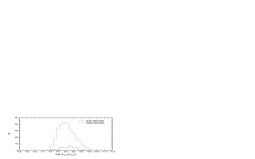
Figure 1: The distribution of $L_{\rm[OIII]}$ for total sample and the sub-sample.

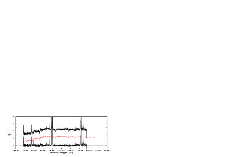
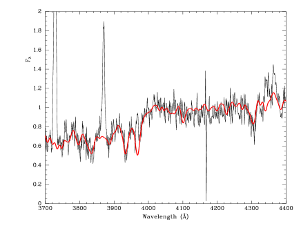
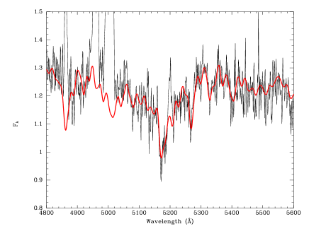
Figure 2: Sample fit of the synthetic population model for SDSS J150117.96+545518.2. Top: the observed spectra (top black curve, shifted up for clarity), the synthetic spectra (middle red curve), and the residual spectrum (bottom black curve). Bottom: the region around Ca H+K $\lambda\lambda$ 3969, 3934 and G-band (left); the region around Mg Ib$\lambda\lambda$ 5167, 5173, 5184 triplet (right).

In order to check whether this sub-sample is representative of the total sample of Zakamsa et al. (2003) with respect to the [O III]$\lambda$5007 luminosity ($L_{\rm[OIII]}$), we plot the histograms of the $L_{\rm[OIII]}$ distribution for the sub-sample and total-sample (see Figure 1). Then T-test shows that these two populations are drawn from the same parent population with a possibility of 0.95. $L_{\rm[OIII]}$ is directly adopted from Table 1 in Zakamsa et al. (2003), the adopted raw $L_{\rm[OIII]}$ values and associated quantities are lower limits. Using the $L_{\rm[OIII]}$ criterion of $3\times 10^{8}\mbox{\,$\rm L_{\odot}$}$(the logarithm is $\sim 8.48$), which corresponds to the intrinsic absolute magnitude $M_{B}<-23$ (Zakamsa et al. 2003), 20 objects can then be classified as type II quasars. Fig. 2 shows a fitting example of for SDSS J150117.96+545518.2 with S/N=20.5. The final results are presented in Table 1. All the fittings for 33 type II AGNs are appended in the Appendix.

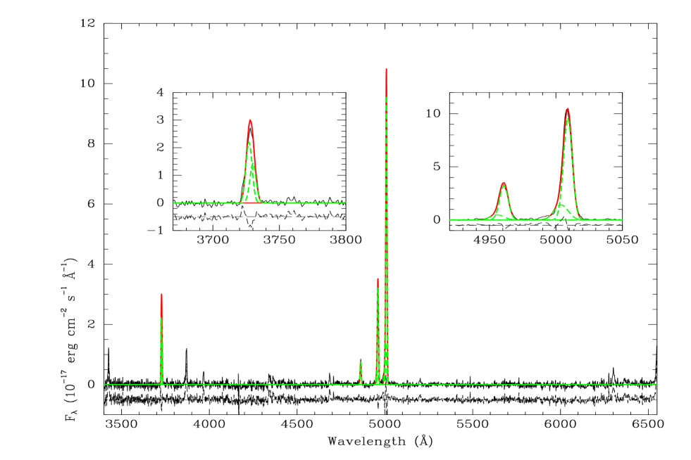
Figure 3: Sample multi-component fitting of the [O II]$\lambda\lambda$3726,3729 and [O III]$\lambda\lambda$4959, 5007 lines for SDSS J150117.96+545518.2: modeled composite profile (thick solid red line), individual components (the dotted green lines), the residual spectrum (lower panel).

After subtracting the synthetic stellar components and the AGNs continuum, we obtain the clean pure emission-line spectra as shown in the top panel of Fig. 2, where we can analyze the pure emission-line profiles in detail by using the multi-component spectral fitting task SPECFIT (Kriss 1994) in the IRAF-STSDAS package . Because of the asymmetric profiles of the [O III]$\lambda\lambda$4959, 5007 lines, two sets of two-gaussian profiles are used in order to remove properly the asymmetric blue/red wings of the [O III] line. We take the same linewidth for each component, and fix the flux ratio of [O III]$\lambda$4959 to [O III]$\lambda$5007 to be 1:3. For three objects, we can’t fit the [O III] lines for their irregular [O III] lines (see Table 1). For the [O II]$\lambda\lambda$ 3727, 3729 lines, we use two-gaussian profiles and fix their wavelength separation to the laboratory value; the ratio of the line intensities is allowed to vary during the fitting. The decomposition for [O II] lines is more difficult because of relatively low S/N and that the expected line widths are comparable to the pair separation (2.4Å). For objects with available H$\alpha$, we also used one-gaussian profile to fit NII $\lambda\lambda$ 6548,6583 and H$\alpha$ 6563 lines. And H$\alpha$ and H$\alpha$ luminosities would be used to do the extinction correction. For more details, please refer to Bian, Yuan & Zhao (2005, 2006). Our sample fitting for SDSS J150117.96+545518.2 is showed in Fig. 3.

3 Results and discussion

3.1 The uncertainties of the stellar velocity dispersion ($\sigma_{*}$) and the gaseous velocity dispersion ($\sigma_{g}$)

The derived stellar velocity dispersion was corrected by the instrumental resolutions of both the SDSS spectra and the STELIB library. Cid Fernandes et al. (2004a) have used their stellar population synthesis method to study a sample of 79 nearby galaxies observable from the southern hemisphere, of which 65 are Seyfert 2 galaxies. The S/N in the S/N window varies between 10 and 67. They compared their $\sigma_{*}$ with values from the literature and found the agreement is good. They estimated that the uncertainty in $\sigma_{*}$ is typically about 20 km s^-1. Recently, Cid Fernandes et al. (2005) applied their synthesis method to a larger sample of 50362 galaxies from the SDSS Data Release 2 (DR2). Their derived $\sigma_{*}$ is consistent very well with that of the MPA/JHU group (Kauffmann et al. 2003). The median of the difference between the two estimates is just 9 km s^-1. We have carefully checked our synthesis fitting result one by one and picked out 33 type II AGNs that are well fitted and the stellar velocity dispersion ($\sigma_{*}$) are reliably derived. The spectral S/N for these objects are in the range of 5 to 21.5, most of which larger than 10, thus the typical uncertainty in $\sigma_{*}$ should be around 20 km s^-1.

Recently, Greene & Ho (2006a, 2006b) used the direct-fitting method (Barth et al. 2002) to study the the systematic biases of $\sigma_{*}$ from different regions around Ca II triplet, Mg Ib triplet, and CaII H+K stellar absorption features, which are introduced by both template mismatch and contamination from AGNs. They argue that the Ca II triplet provides the most reliable measurements of $\sigma_{*}$ and there is a systematic offset between $\sigma_{\rm CaK}$ and $\sigma_{*}$ derived from other spectral regions. For our higher-redhsift sample and the SDSS wavelength coverage 3800-9200Å, it is impossible to measure $\sigma_{*}$ from Ca II triplet. Therefore, for higher-redhsift type II AGNs, new observations around Ca II triplet are necessary in the future. Here we used the following formula to obtain the corrected velocity dispersion $\sigma_{*}^{c}$ (Greene & Ho 2006b),

$$\sigma_{*}^{c}=(1.40\pm 0.04)\sigma_{*}-(71\pm 5).$$ (2)

For three objects, $\sigma_{*}$ is near the instrumental resolution and the corrected $\sigma_{*}^{c}$ is unreliable. These objects are excluded from further analysis, and denoted as ${\dagger}$ in Table 1.

The gaseous velocity dispersion ($\sigma_{\rm g}$) is obtained from full width half maximum (FWHM) of emission lines by assuming the Gaussian profile: $\rm\sigma_{\rm[OII]}^{g}=FWHM[OII]/2.35$ and $\rm\sigma_{\rm[OIII]}^{g}=FWHM[OIII]/2.35$. Taking into account the SDSS spectrum resolution, the intrinsic $\sigma_{g}$ derived from $\rm FWHM([OIII])$ may be instrumentally broadened. The intrinsic $\sigma_{\rm g}$ value can be approximated by $\sigma_{\rm g}=(\sigma_{\rm obs}^{2}-(\sigma_{\rm inst}/(1+z))^{2})^{1/2}$, where z is the redshift. For the spectra from SDSS, the mean values of $\sigma_{\rm inst}$ are 74 km s^-1(the logarithm is 1.87 dex) for [O II], and 60 km s^-1(the logarithm is 1.78 dex) for [O III] (Greene & Ho 2005), respectively. The results of $\sigma_{\rm g}$ are listed in Table 1 (columns 7 and 8). After removing the effect of instrumental broadening, some objects become unresolved (see Table 1). Measurements of $\sigma_{\rm g}$ below the resolution limit (74 and 60 km s^-1for [O II] and [O III], respectively) are not reliable. The error of $\sigma_{\rm g}$ is derived from the measurement error of the linewidth. For the linewidth, the typical error is about 10 per cent. However, the systematic effects are neglected, e.g. the uncertainties of the continuum subtraction and component decomposition (Bian, Yuan & Zhao 2005).

3.2 The extinction correction of the [O III]$\lambda$5007 luminosity

The [O III] line has the advantage of being strong and easy to detect in AGNs. The [O III]$\lambda$5007 line is usually used as a tracer of AGNs activity (e.g. Heckman et al., 2004; Greene & Ho 2005). However, the [O III]$\lambda$5007 luminosity is subject to extinction by interstellar dust in the host galaxy and in our Galaxy. Using SDSS data, Kauffmann et al (2003) found that for type II AGNs at $z<0.3$ the mean value of the ratio of the corrected luminosity to the observational luminosity ($log(\frac{L^{c}_{[OIII]}}{L_{[OIII]}})$, the extinction factor at 5007$\AA$) is about 0.85 dex and suggested that the extinction effect should be huge for type II quasars. The extinction correction is usually corrected by using the Balmer decrement, which is regarded as the best approximation. For 18 out of these 33 objects with available H$\alpha$ measurements in the stellar-light subtracted spectra, we calculated the extinction correction of the [O III]$\lambda$5007 luminosity, from the relation (Bassani et al. 1999)

$$L_{\rm[OIII]}^{\rm c}=L_{\rm[OIII]}\rm[\frac{(H_{\alpha}/H_{\beta})_{obs}}{(H_{\alpha}/H_{\beta})_{0}}]^{2.94}$$ (3)

where an intrinsic Balmer decrement $\rm(H_{\alpha}/H_{\beta})_{0}=3.0$ is adopted (Gu & Huang 2002). The range of the extinction factors at [OIII] is between -0.24 dex and 1.25 dex. The extinction-corrected [O III]$\lambda$5007 luminosity is listed in Col. 11 in Table 1. If we used the $L_{\rm[OIII]}$ criterion of $3\times 10^{8}\mbox{\,$\rm L_{\odot}$}$ (Zakamsa et al. 2003), 14 out of these 18 objects can then be classified as type II quasars.

Using the SDSS AGN catalogue at MPA/JHU (Kauffmann et al 2003), we obtained the extinction factor at 5007$\AA$, $log(\frac{L^{c}_{[OIII]}}{L_{[OIII}})$. We tried to obtain a relation between $\frac{L^{c}_{[OIII]}}{L_{[OIII}}$ and other observational parameters, such as $\sigma_{*}$, $L_{[OIII}]$, $L_{H\beta}$. However, no correlation is found. More careful work is required to deal with this problem in the future.

3.3 The SMBHs masses and Eddington ratios in type II quasars

Using the reverberation mapping method or the empirical size-luminosity relation, it is impossible to estimate the SMBHs masses in type II quasars for the lack of emission lines from BLRs. Here we use the formulae to derive the SMBHs masses in type II quasars from the stellar velocity dispersion $\sigma_{*}$ (Tremaine et al. 2002), which is $M_{\rm BH}(\mbox{\,$\rm M_{\odot}$})=10^{8.13}(\sigma_{*}^{c}/(200\ \rm kms^{-1}))^{4.02}$.

We calculate the Eddington ratio, $L_{\rm bol}/L_{\rm Edd}$. We use the extinction-corrected [O III] luminosity ($L^{c}_{[OIII}$) as a surrogate for the AGNs luminosity (Heckman et al., 2004; Greene & Ho 2005), $\rm L_{\rm bol}=3500L^{\rm c}_{\rm[OIII]}$, to calculate the bolometric luminosity $L_{\rm bol}$, and $\rm L_{\rm Edd}=1.26\times 10^{38}M_{\rm BH}/\mbox{\,$\rm M_{\odot}$}~{}ergs~{}s^{-1}$. Objects with no extinction corrected [O III] luminosity are discarded in the analysis relative to the Eddington ratio. The results of SMBHs masses and Eddington ratios in type II AGNs are also presented in Table 1 (columns 13 and 14). We also calculate the SMBHs masses and Eddington ratios for the lower-redshifts type II AGNs at $0.02<z<0.3$ presented by Kauffmann et al. (2003). For the typical uncertainties of 20km s^-1for $\sigma_{*}=200$ km s^-1, the errors of $log~{}\sigma_{*}$ would be about 0.05 dex, corresponding 0.17 dex for $logM_{\rm BH}$, and almost the same for $L_{\rm bol}/L_{\rm Edd}$ (Bian, Yuan, & Zhao 2005). Here we don’t consider the cosmology evolution of $M_{\rm BH}-\sigma_{*}$ relation (e.g. Woo et al. 2006), which is a question open to debate.

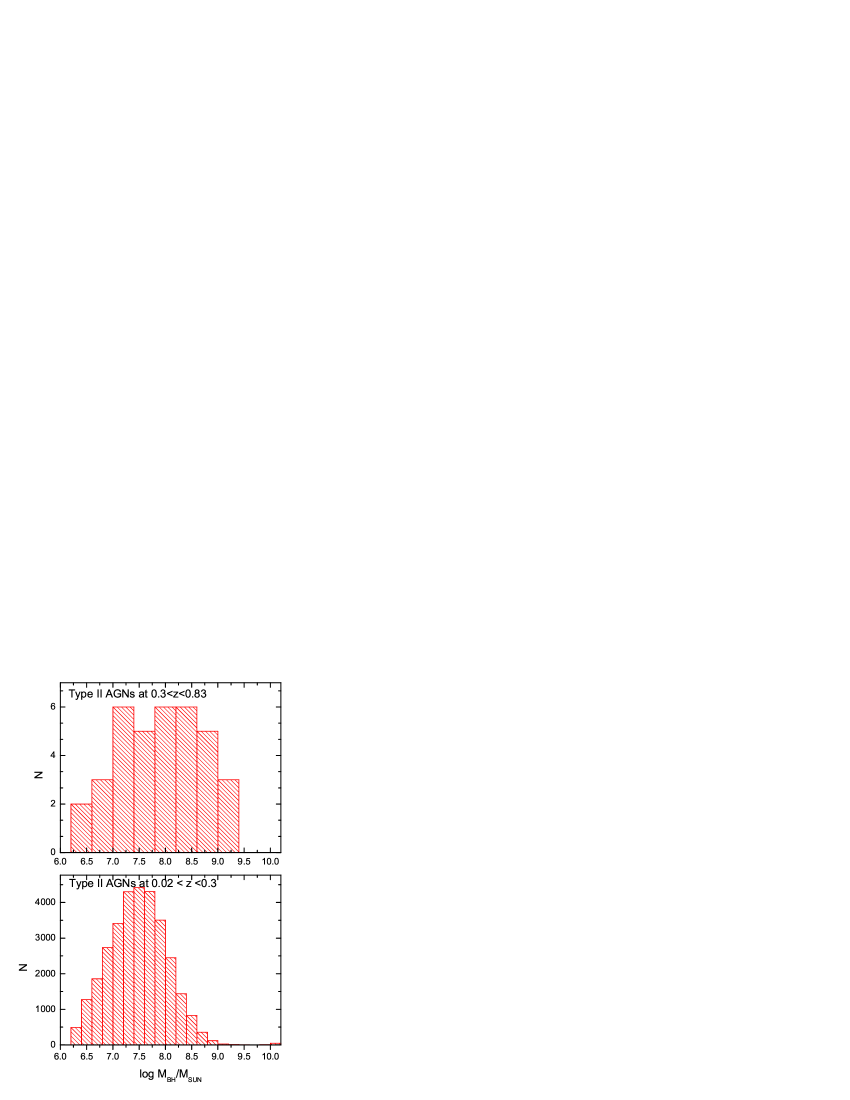
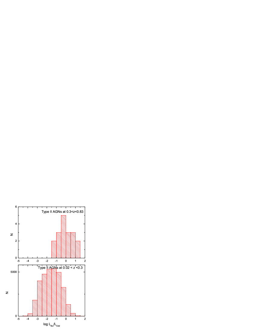
Figure 4: The distribution of SMBHs masses and Eddington ratios for our results (type II AGNs at $0.3<z<0.83$) and for Kaufmann et al. (2003, type II AGNs at $0.02<z<0.3$)).

In Fig. 4, we compare the distribution of SMBHs masses and Eddington ratios in the lower-redshifts sample and the higher-redshifts sample. It is found that the type II AGNs at higher-redshifts have higher SMBHs masses and higher Eddington ratios.

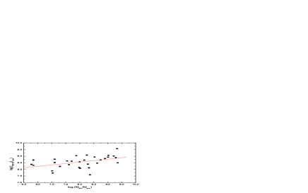
Figure 5: The [O III] luminosity (left) and the corrected [O III] luminosity (right) plotted against the SMBHs masses derived from the stellar velocity dispersion $\sigma$. Solid line is the best fit.

It is well known that the Eddington ratio is an important parameter to describe the accretion process in AGNs. The [O III] luminosity is usually used as a surrogate for the AGNs luminosity (Heckman et al. 2004 and the reference therein). In Fig. 5, we plot the [O III] luminosity and the corrected [O III] luminosity versus the SMBHs masses. Using a least-squares regression, we derive the correlation between $M_{\rm BH}$ and $L_{\rm[OIII]}$ to be: $\rm log(L_{[OIII]}/L_{\odot})=(6.83\pm 0.65)+(0.22\pm 0.08)log(M_{BH}/M_{\odot})$. The correlation coefficient R is 0.45, with a probability of $P_{null}=0.012$ for rejecting the null hypothesis of no correlation. However, no correlation is found between $M_{\rm BH}$ and $L^{c}_{\rm[OIII]}$. No correlation is found between the Eddington ratio and the [O III] luminosity or the corrected [O III] luminosity. From the photoionization model, the strength of [O III] is controlled by the NLRs covering factor, density, and ionization parameter (e.g. Baskin & Laro 2005). The relation between the [O III] luminosity and the AGNs bolometric luminosity is still a question to debate.

3.4 The $\sigma_{\rm g}-\sigma_{*}$ relation

The existence of a good correlation between stellar velocity dispersion ($\sigma_{*}$) and ionized gas velocity dispersion ($\sigma_{\rm g}$) (e.g. Nelson & Whittle 1996) suggests that the gaseous kinematics of NLRs in Seyfert galaxies be primarily dominated by the bulge gravitational potential, which is further confirmed by Nelson & Whittle (1996). Most recently, Greene & Ho (2005) have investigated a large and homogeneous sample of lower-redshift (0.02 $<$ z $<$ 0.3) Type II AGNs from the SDSS, and found that $\sigma_{\rm g}$ traces $\sigma_{*}$. Though the gas kinematics of NLRs are governed by the gravitational potential of the bulges, they also find that the accretion rate plays an important secondary role.

Following Greene & Ho (2005), we study the $\sigma_{\rm g}-\sigma_{*}^{c}$ relation for 33 Type II AGNs at redshifts 0.3 $<$ z $<$ 0.83 after measuring the gas velocity dispersion ($\sigma_{\rm g}$) from the narrow emission lines from NLRs, and the stellar velocity dispersion ($\sigma_{*}^{c}$) from the CaII H+K, G-band absorption feature, which is shown in Fig. 2. In Fig. 6, we showed the relation between $\sigma_{g}$ and $\sigma_{*}^{c}$. The correlation coefficients are 0.19, 0.27, 0.70, 0.54 for figurs in Fig. 6, from left to right and from top to bottom. The relation between $\sigma_{g}$ and $\sigma_{*}^{c}$ becomes much weaker at higher redshifts. We also found that this poor correlation is not due to the S/N. In order to qualify the comparison between $\sigma_{\rm g}$ and $\sigma_{*}^{c}$, we calculate the distribution of $<\sigma_{\rm g}/\sigma_{*}^{c}>$. The value is $1.24\pm 0.76$ for the the core component of [O III] line, $1.20\pm 0.96$ for the [O II] line. These suggest that $\sigma_{\rm g}$ of the the core component of [O III] and [O II] lines can trace $\sigma_{*}^{c}$ within 0.09 and 0.08 dex in the logarithm of $\sigma_{*}^{c}$, respectively, and that the high-ionization [O III] line traces $\sigma_{*}^{c}$ as well as the low-ionization [O II] line. If we use the line width of [O III] core component to estimate the SMBHs masses from the Tremaine’s M${}_{\rm BH}-\sigma$ relation, we would overestimate SMBHs masses by about 0.38 dex.

For comparison, Greene & Ho (2005) derived the distribution of $<\sigma_{\rm g}/\sigma_{*}>$ of lower-redshift type II AGNs with $0.02<z<0.3$, which are $1.34\pm 0.66$ for the [O III] line, $1.00\pm 0.35$ for the [O III] core line, and $1.13\pm 0.38$ for the [O II] line. We also calculate the the distribution of $<\sigma_{\rm g}/\sigma_{*}^{c}>$ for the sample of Seyfert galaxies (Nelson & Whittle 1996); the value is $1.15\pm 0.68$, suggesting that $\sigma_{\rm g}$ of the [O III] line can trace $\sigma_{*}^{c}$ within 0.06 dex in the logarithm of $\sigma_{*}^{c}$ . Our results are thus consistent with theirs.

To a first-order approximation, the line widths of the core component of [O III] and [O II] for both low-redshift and high-redshift Type II AGNs are primarily controlled by the gravitational potential of the bulges of host galaxies, and can approximately trace the stellar velocity dispersion. As we know, the errors in virial SMBHs masses derived from galaxy dynamics or size-luminosity relation is about  0.5 dex (e.g. Magorrian et al. 1998; Kaspi et al. 2000; Bian & Zhao 2004a, 2004b). We also can use the line-width of the core component of [O III] or [O II] to estimate the black hole mass.

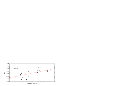
Figure 7: $\Delta\sigma=log\sigma_{g}-log\sigma_{*}^{c}$ plotted against the Eddington ratio, $L_{bol}/L_{Edd}$. Left panel is for the [O III] line and right panel is for the [O II] line. Solid lines show the best fits.

In order to find the secondary effect of the line broadening in gas lines from NLRs for our higher-redshift narrow-line AGNs, we studied the relation between the deviation of $\sigma_{\rm g}$ from $\sigma_{*}^{c}$ ($\Delta\sigma=log\sigma_{\rm g}-log\sigma_{*}^{c}$) and the Eddington ratio ($L_{\rm bol}/L_{\rm Edd}$) (Greene & Ho 2005). Using the least-square regression, we find a median strong correlation between these two dimensionless parameters. For the [O III] line, the relation is: $\Delta\sigma=(-0.035\pm 0.057)+(0.202\pm 0.058)log(L_{\rm bol}/L_{\rm Edd})$, R=0.71, $P_{\rm null}=0.00441$. For the [O II] line, the relation is $\Delta\sigma=(0.047\pm 0.058)+(0.179\pm 0.059)log(L_{\rm bol}/L_{\rm Edd})$, R=0.65, $P_{\rm null}=0.0091$ (see Fig. 7). We also find the comparable correlation between $\Delta\sigma$ and $M_{\rm BH}$. These results confirm that the nuclei accretion process and/or nuclei SMBHs would affect the linewidth of gas lines from NLRs, although the primary driver is the gravitational potential of the bulge.

4 Conclusion

The stellar population synthesis code is used to model the stellar contribution for a sample of 209 type II AGNs at redshifts $0.3<z<0.83$ from SDSS. According to the $L_{\rm[OIII]}$ criterion of $3\times 10^{8}\mbox{\,$\rm L_{\odot}$}$, 20 can be classified as type II quasars. The main conclusions can be summarized as follows.

• The reliable $\sigma_{*}$ are measured for 33 type II AGNs with significant stellar absorption features. We use the formula of Greene & Ho to obtain the corrected stellar velocity dispersions ($\sigma_{*}^{c}$ and SMBHs masses are calculated from the $M_{\rm BH}-\sigma_{*}^{c}$ relation. A median strong relation between the [O III] luminosity and the SMBH mass is found (although no correlation between the extinction-corrected [O III] luminosity and the SMBH mass); no correlation is found between the Eddington ratio and the [O III] luminosity or the extinction-corrected [O III] luminosity.

• The gas velocity dispersion ($\sigma_{g}$) in NLRs is measured using three sets of two-gaussian profiles to fit [O III]$\lambda\lambda$4959, 5007 and [O II]$\lambda\lambda$3727, 3729) in these 33 stellar-light subtracted spectra. We find that the relation between $\sigma_{g}$ and $\sigma_{*}^{c}$ becomes much weaker at higher redshifts.

• The distribution of $<\sigma_{g}/\sigma_{*}^{c}>$ is $1.24\pm 0.76$ for the core [O III] line and $1.20\pm 0.96$ for the [O II] line, which suggests that $\sigma_{g}$ can trace $\sigma_{*}^{c}$ within about 0.1 dex in the logarithm of $\sigma_{*}^{c}$. The deviation of $\sigma_{g}$ from $\sigma_{*}^{c}$ is correlated with the Eddington ratio.

name	z	$\sigma_{*}$	$[OIII]$	$[OII]$	$\sigma_{*}^{c}$	$\sigma_{g}^{[OIII]}$	$\sigma_{g}^{[OII]}$	$L_{[OIII]}$	$L_{[OII]}$	$L^{c}_{[OIII]}$	S/N	$M_{bh}$	$\frac{L_{bol}}{L_{Edd}}$
(1)	(2)	(3)	(4)	(5)	(6)	(7)	(8)	(9)	(10)	(11)	(12)	(13)	(14)
SDSS J113344.02+613455.7	0.426	273	$327\pm 98$	$526\pm 71$	2.49	$2.13^{+0.12}_{-0.18}$	$2.34^{+0.06}_{-0.07}$	8.82	8.52	–	21.5	8.90	–
SDSS J150117.96+545518.2	0.338	289	$456\pm 48$	$436\pm 45$	2.52	$2.28^{+0.05}_{-0.05}$	$2.25^{+0.04}_{-0.05}$	9.06	8.42	8.97	20.5	9.02	-0.81
SDSS J094820.38+582526.4	0.324	126	$470\pm 67$	$750\pm 56$	2.02	$2.29^{+0.06}_{-0.07}$	$2.50^{+0.03}_{-0.03}$	7.89	8.25	9.08	20.2	7.01	0.54
SDSS J002531.45-104022.2	0.303	82	$485\pm 60$	$529\pm 55$	1.64${\dagger}$	$2.31^{+0.05}_{-0.06}$	$2.34^{+0.04}_{-0.05}$	8.73	9.02	8.57	16.7	5.48	2.53
SDSS J083945.98+384319.0	0.424	196	$597\pm 51$	$723\pm 58$	2.31	$2.40^{+0.04}_{-0.04}$	$2.48^{+0.03}_{-0.04}$	8.70	8.40	–	16.1	8.16	–
SDSS J104505.39+561118.3	0.428	204	$413\pm 116$	$505\pm 47$	2.33	$2.23^{+0.11}_{-0.15}$	$2.32^{+0.04}_{-0.04}$	9.08	8.86	–	15.8	8.25	–
SDSS J090414.10-002144.9	0.353	287	$409\pm 49$	$297\pm 32$	2.52	$2.23^{+0.05}_{-0.06}$	$2.06^{+0.05}_{-0.06}$	8.93	8.10	9.03	15.4	9.01	-0.91
SDSS J143027.66-005614.8	0.318	157	$367\pm 118$	$453\pm 59$	2.17	$2.18^{+0.13}_{-0.19}$	$2.27^{+0.06}_{-0.06}$	8.36	7.87	9.23	14.8	7.61	0.48
SDSS J133633.65-003936.4	0.416	153	$486\pm 181$	$470\pm 94$	2.16	$2.31^{+0.14}_{-0.22}$	$2.29^{+0.08}_{-0.10}$	8.64	7.84	–	14.8	7.55	–
SDSS J100459.41+030202.0	0.469	130	$326\pm 13$	$369\pm 57$	2.05	$2.13^{+0.02}_{-0.02}$	$2.17^{+0.07}_{-0.08}$	8.77	8.25	–	14.8	7.10	–
SDSS J020234.55-093921.8	0.302	211	$466\pm 41$	$524\pm 68$	2.35	$2.29^{+0.04}_{-0.04}$	$2.33^{+0.05}_{-0.06}$	8.12	7.80	8.52	14.0	8.33	-1.09
SDSS J094209.00+570019.7	0.35	102	$597\pm 24$	$343\pm 58$	1.86	$2.40^{+0.02}_{-0.02}$	$2.13^{+0.07}_{-0.09}$	8.31	8.34	8.82	12.8	6.34	1.33
SDSS J154337.81-004420.0	0.311	207	$200\pm 39$	$482\pm 60$	2.34	$1.87^{+0.10}_{-0.14}$	$2.29^{+0.05}_{-0.06}$	8.40	7.76	8.33	11.9	8.29	-1.01
SDSS J033606.70-000754.7	0.431	102	$774\pm 52$	$562\pm 82$	1.86	$2.51^{+0.03}_{-0.03}$	$2.37^{+0.06}_{-0.07}$	8.71	7.98	–	11.8	6.34	–
SDSS J075607.15+461411.5	0.593	316	$322\pm 60$	$319\pm 279$	2.57	$2.12^{+0.08}_{-0.10}$	$2.11^{+0.28}_{-1.20}$	9.01	8.18	–	10.8	9.21	–
SDSS J084041.05+383819.9	0.313	163	$720\pm 48$	$650\pm 94$	2.20	$2.48^{+0.03}_{-0.03}$	$2.43^{+0.06}_{-0.07}$	8.62	8.03	9.48	10.8	7.71	0.45
SDSS J143928.23+001538.0	0.339	184	$569\pm 56$	$652\pm 58$	2.27	$2.38^{+0.04}_{-0.05}$	$2.43^{+0.04}_{-0.04}$	8.08	7.99	9.22	10.8	8.01	-0.29
SDSS J231755.35+145349.3	0.311	48	$229\pm 6$	$264\pm 54$	—- ${\dagger}$	$1.94^{+0.01}_{-0.01}$	$1.99^{+0.09}_{-0.12}$	8.10	7.66	8.39	10.7	-	–
SDSS J121856.41+611922.6	0.369	100	$182\pm 28$	$270\pm 27$	1.84	$1.82^{+0.08}_{-0.11}$	$2.01^{+0.05}_{-0.05}$	8.38	8.07	8.60	10.7	6.27	1.33
SDSS J075920.21+351903.4	0.328	214	—	$569\pm 88$	2.36	—	$2.37^{+0.06}_{-0.08}$	7.59	7.88	8.84	10.4	8.36	-0.91
SDSS J132529.32+592424.9	0.429	328	$443\pm 61$	$441\pm 42$	2.59	$2.27^{+0.06}_{-0.07}$	$2.26^{+0.04}_{-0.05}$	8.89	8.37	–	10.2	9.29	–
SDSS J090626.80+033310.7	0.363	127	$191\pm 36$	$271\pm 70$	2.03	$1.85^{+0.10}_{-0.13}$	$2.01^{+0.11}_{-0.16}$	7.73	7.17	–	10.2	7.03	–
SDSS J031012.82-010822.6	0.303	70	$200\pm 51$	$242\pm 68$	1.43${\dagger}$	$1.87^{+0.12}_{-0.20}$	$1.93^{+0.12}_{-0.19}$	8.06	7.73	8.40	10.1	4.63	2.74
SDSS J092318.04+010144.7	0.386	230	$694\pm 64$	$406\pm 68$	2.40	$2.47^{+0.04}_{-0.04}$	$2.22^{+0.07}_{-0.09}$	8.94	7.94	9.31	9.9	8.53	-0.34
SDSS J081507.42+430427.1	0.510	335	$860\pm 35$	$1070\pm 76$	2.60	$2.56^{+0.02}_{-0.02}$	$2.66^{+0.03}_{-0.03}$	9.57	9.02	–	9.8	9.33	–
SDSS J033248.49-001012.3	0.310	339	$627\pm 117$	$672\pm 55$	2.61	$2.42^{+0.08}_{-0.09}$	$2.45^{+0.03}_{-0.04}$	8.50	7.97	8.26	9.6	9.36	-2.23
SDSS J092014.11+453157.3	0.402	174	$666\pm 50$	$447\pm 70$	2.24	$2.45^{+0.03}_{-0.03}$	$2.26^{+0.07}_{-0.08}$	9.04	8.43	–	9.6	7.87	–
SDSS J214415.61+125503.0	0.390	182	$426\pm 43$	$614\pm 124$	2.26	$2.25^{+0.04}_{-0.05}$	$2.41^{+0.08}_{-0.10}$	8.14	7.81	–	8.6	7.98	–
SDSS J153943.73+514221.0	0.585	240	$427\pm 43$	$349\pm 79$	2.42	$2.25^{+0.04}_{-0.05}$	$2.15^{+0.09}_{-0.12}$	8.47	8.37	–	8.5	8.62	–
SDSS J133735.01-012815.6	0.329	254	$331\pm 130$	$265\pm 264$	2.45	$2.13^{+0.15}_{-0.26}$	$1.99^{+0.33}_{-1.20}$	8.72	8.28	9.56	6.8	8.75	-0.49
SDSS J165627.28+351401.7	0.679	183	—	$573\pm 66$	2.27	—	$2.38^{+0.05}_{-0.05}$	8.57	7.91	–	6.7	8.00	–
SDSS J101237.29+023554.3	0.720	139	—	$799\pm 98$	2.09	—	$2.53^{+0.05}_{-0.06}$	8.22	8.19	–	5.1	7.29	–
SDSS J094836.03+002104.5	0.324	130	$555\pm 116$	$515\pm 40$	2.05	$2.37^{+0.08}_{-0.11}$	$2.33^{+0.03}_{-0.04}$	8.52	7.90	8.81	4.9	7.10	0.62

Table 1: Results for type II quasars, sorted by the value of S/N. The columns are as follows: (1) name; (2) redshift; (3) uncorrected stellar velocity dispersion in units of km s^-1; (4) FWHM of [O III]$\lambda$ 5007 Å in units of km s^-1; (5) FWHM of [O II]$\lambda$ 3727 Å in units of km s^-1; (6) log of corrected stellar velocity dispersion by equation 2 (in units of km s^-1); (7) log of the [O III] $\sigma$ in units of km s^-1; (8) log of the [O II] $\sigma$ in units of km s^-1; (9) log of [O III] luminosity in unit of  $\rm L_{\odot}$; (10) log of [O II] luminosity in unit of  $\rm L_{\odot}$; (11) log of extinction-corrected [O II] luminosity in unit of  $\rm L_{\odot}$; (12) signal-to-noise ratio (S/N); (13) log of the black hole mass in units of solar mass; (14) log of the Eddington ratio. ${\dagger}$: $\sigma_{*}$ is near the instrumental resolution and the corrected $\sigma_{*}^{c}$ is unreliable, which is excluded from future analysis.

Figure 6: Top left panel is $\sigma_{g}$ versus $\sigma_{*}^{c}$ for the [O III] line; top right panel is $\sigma_{g}$ versus $\sigma_{*}^{c}$ for the [O II] line; bottom left is $\sigma_{g}^{[OIII]}$ versus $\sigma_{g}^{[OII]}$; bottom right is $\sigma_{g}$ versus $\sigma_{*}$ for the the sample of Nelson & Whittle (1996). The uncertainty in $\sigma$ is typically 20 km s^-1. The solid line denotes 1:1.

References

- [] Antonucci R., 1993, ARA&A, 31, 473
- [] Barth A. J., Ho L. C., & Sargent W. L. W., 2002, AJ, 124, 2607
- [] Begelman M. C., 2003, Science, 300, 1898
- [] Baskin A., Laro A., 2005, MNRAS, 358, 1043
- [] Bassani L., et al., 1999, ApJS, 121, 473
- [] Bian W., Zhao Y., 2004a, MNRAS, 347, 607
- [] Bian W., Zhao Y., 2004b, MNRAS, 352, 823
- [] Bian W., Yuan Q., Zhao Y., 2005, MNRAS, 364, 187
- [] Bian W., Yuan Q., Zhao Y., 2006, MNRAS, 367, 860
- [] Brinchmann J., et al., 2004, ApJ, 613, 109
- [] Bruzual G., Charlot S., 2003, MNRAS, 344, 1000
- [] Cardelli J. A., Clayton G. C., Mathis J. S., 1989, ApJ, 345, 245
- [] Cid Fernandes R., Sodre L., Schmitt H. R., Leao J. R. S., 2001, MNRAS, 325, 60
- [] Cid Fernandes R., Gu Q., Melnick J., et al., 2004a, MNRAS, 355, 273
- [] Cid Fernandes R., Gonzalez Delgado R., Storchi-Bergmann, T., Pires Martins, L., Schmitt H., 2004b, MNRAS, 356, 270
- [] Cid Fernandes R., Mateus A., Sodre L., Stasinska G., Gomes J., 2005, MNRAS, 358, 363
- [] Ferrarese, L., Merritt D. 2000, ApJ, 539, L9
- [] Gebhardt K., et al. 2000, ApJ, 539, L13
- [] Greene J. E., Ho L. C., 2005, ApJ, 627, 721
- [] Greene J. E., Ho L. C., 2006a, ApJL, 641, L21
- [] Greene J. E., Ho L. C., 2006b, ApJ, 641, 117
- [] Gu Q., Huang J., 2002, ApJ, 579, 205
- [] Gu Q., Melnick J., Cid Fernandes R., Kunth D., Terlevich, Terlevich R., et al. 2006, MNRAS, 366, 480
- [] Heckman T. M., et al., 2004, ApJ, 613, 109
- [] Kaspi S., Smith P.S., Netzer H., Maoz D., Jannuzi B.T., Giveon U., 2000, ApJ, 533, 631
- [] Kauffmann G., et al. 2003, MNRAS, 346, 1055
- [] Kauffmann, G., & Heckman, T. M. 2005, Philos. Trans. R. Soc. London, A363, 621
- [] Koski A. T., 1978, ApJ, 223, 56
- [] Kriss G. A. 1994, in ASP Conf. Ser. 61, Astronomical Data Analysis Software and Systems III, ed. Crabtree D. R., Hanisch R. J., Barnes J. (San Francisco: ASP), 437
- [] Maggorian J., et al., 1998, AJ, 115, 2285
- [] McLure R. J., Jarvis M. J., 2002, MNRAS, 337, 109
- [] Nelson C. H., 2001, ApJ, 544, L91
- [] Nelson C. H., Whittle M., 1996, ApJ, 465, 96
- [] Rix H. W., & White S. D. M. 1992, MNRAS, 254, 389
- [] Sargent W. L. W., Schechter P. L., Boksenberg A., & Shortridge K. 1977, ApJ, 212, 326
- [] Schlegel D. J., Finkbeiner D. P., Davis M., 1998, ApJ, 500, 525
- [] Shen Z. Q., et al., Nature, 2005, 438, 62
- [] Tonry J., & Davis M., 1979, ApJ, 84, 1511
- [] Tremaine S., et al., 2002, Ap J, 574, 740
- [] Urry C. M., Padovani P., 1995, PASP, 107, 803
- [] Vestergaard M., 2002, ApJ, 571, 733
- [] Watanabe M., et al., 2003, ApJ, 591, 714
- [] Woo J. H., et al., 2006, ApJ, in press, astro-ph/0603648
- [] Wu X. B., et al., 2004, A& A, 424, 793
- [] Zakamsa N. L., et al., 2003, AJ, 126, 2125