Cleaned Three-Year WMAP CMB Map: Magnitude of the Quadrupole and Alignment of Large Scale Modes

Abstract

We have produced a cleaned map of the Wilkinson Microwave Anisotropy Probe (WMAP) three-year data using an improved foreground subtraction technique. We perform an internal linear combination (ILC) to subtract the Galactic foreground emission from the temperature fluctuations observed by the WMAP. We divide the whole sky into hundreds of pixel groups with similar foreground spectral indices over a range of WMAP frequencies, apply the ILC for each group, and obtain a CMB map with foreground emission effectively reduced. With the resulting foreground-reduced ILC map (Figure 4$b$, available on-line), we have investigated the known anomalies in CMB maps at large scales, namely the low quadrupole ($l=2$) power, and the strong alignment and planarity of the quadrupole and the octopole ($l=3$). Our estimates are consistent with the previous measurements. The quadrupole and the octopole powers measured from our ILC map are $\delta T_{2}^{2}=276_{-126}^{+94}~{}\mu\textrm{K}^{2}$ and $\delta T_{3}^{2}=952_{-83}^{+64}~{}\mu\textrm{K}^{2}$, respectively. The 68% confidence limits are estimated from the ILC simulations and include the cosmic variance. The measured quadrupole power is lower than the value expected in the concordance $\Lambda$CDM model ($1250~{}\mu\textrm{K}^{2}$), in which the probability of finding a quadrupole power lower than the measured value is $5.7$%. We have confirmed that the quadrupole and the octopole are strongly aligned with angle $\theta_{23}=11\fdg 8_{-8\fdg 0}^{+6\fdg 4}$, and are planar with high planarity parameters $t=0.98_{-0.02}^{+0.02}$ for $l=2$ and $t=0.91_{-0.03}^{+0.02}$ for $l=3$. The observed angular separation $\theta_{23}$ is marginally statistically significant because the probability of finding the angular separation as low as the observed value is 4.3%. However, the observed planarity is not statistically significant. The probability of observing such a planarity as high as the measured $t$ values is over 18%. The ILC simulations show that the residual foreground emission in the ILC map does not affect the estimated values significantly. The large scale modes ($l=2$–$8$) of SILC400 shows anti-correlation with the Galactic foreground emission on the southern hemisphere. It is not clear whether such anti-correlation occurs due to the residual Galactic emission or by chance.

1. Introduction

The Wilkinson Microwave Anisotropy Probe (WMAP; Bennett et al. 2003a) has measured the cosmic microwave background (CMB) temperature anisotropy and polarization with high resolution and sensitivity, and opened a new window to precision cosmology. The WMAP one-year data imply that the observed CMB fluctuations are consistent with predictions of the concordance $\Lambda\textrm{CDM}$ model with scale-invariant adiabatic fluctuations generated during the inflationary epoch (Hinshaw et al., 2003; Kogut et al., 2003; Spergel et al., 2003; Page et al., 2003; Peiris et al., 2003). The recent release of the WMAP three-year data has confirmed the primary results from the one-year data, giving more accurate determination of cosmological parameters (Hinshaw et al., 2006; Spergel et al., 2006; Page et al., 2006).

However, some peculiar aspects of the CMB maps have been noticed, leading to many controversies. First, there have been many reports of detection of non-Gaussian signatures (Chiang et al. 2003; Park 2004; Eriksen et al. 2004b, c; Coles et al. 2004; Copi et al. 2004; Vielva et al. 2004; Cruz et al. 2005, 2006; Tojeiro et al. 2006), as opposed to the WMAP team’s result (Komatsu et al., 2003; Spergel et al., 2006). In particular, the origin of the asymmetry in statistical properties of the CMB between the Galactic northern and southern hemispheres (Park 2004; Eriksen et al. 2004b) has not been fully explained. Freeman et al. (2006) have studied the effects of the map-making algorithm on the observed asymmetry in CMB temperatures between the Galactic northern and southern hemispheres in the WMAP data. Another interesting issue is the low CMB quadrupole power. Cut-sky analysis of WMAP three-year data gives a quadrupole power of $211~{}\mu\textrm{K}^{2}$, which is quite a bit lower than the expected value in the best-fit $\Lambda\textrm{CDM}$ model ($1250~{}\mu\textrm{K}^{2}$; Hinshaw et al. 2006; Spergel et al. 2006). Through subsequent analyses of the WMAP data, such a low quadrupole power has been confirmed and the effect of the residual foreground emission on the statistical properties of CMB has been extensively studied (e.g., Tegmark et al. 2003; Efstathiou 2004; Eriksen et al. 2004a; Bielewicz et al. 2004, 2005; Slosar & Seljak 2004; Slosar, Seljak, & Makarov 2004; Naselsky et al. 2006; de Oliveira-Costa & Tegmark 2006). The alignment and planarity of $l=2$ and $3$ modes on the sky are also interesting features that have been seen in the WMAP data (de Oliveira-Costa et al., 2004; Schwarz et al., 2004; Land & Magueijo, 2005; Copi et al., 2006; Abramo et al., 2006).

Although each of the anomalies in the CMB anisotropy may have its own cosmological origin, there is a possibility that the residual Galactic foreground emission has affected the nature of the observed temperature fluctuations. Therefore, foreground subtraction is very important as a starting point of all CMB-related analyses. The most popular method of foreground removal is to model the Galactic emission as the weighted sum of foreground templates such as synchrotron, free-free, and dust emission maps (e.g., Bennett et al. 2003b). Another method of foreground removal is the internal linear combination (ILC) method using multi-frequency data (Brandt et al., 1994; Tegmark & Efstathiou, 1996; Bennett et al., 2003b).

The WMAP team has created the ILC map (hereafter WILC1YR) by computing a weighted combination of the WMAP maps that have been band averaged within each of the five WMAP frequency bands, all smoothed to $1\arcdeg$ resolution (Bennett et al., 2003b). The weights are determined by minimizing the variance of temperatures in the combined map, with a constraint that the sum of the weights is one. They have defined twelve disjoint regions on the sky, within which weights are determined independently. Except for the biggest Kp2 region, the other 11 regions are defined by subdividing the inner Galactic plane with lines of constant Galactic longitudes. However, the combination weights found by the WMAP team do not give the minimum variance, and their method of ‘non-linear searching’ for the set of weights has not been described.

Eriksen et al. (2004a) have improved the WMAP team’s ILC method by applying a Lagrange multiplier to produce a variance-minimized ILC map (hereafter LILC). They use the same 12 disjoint regions and the smoothing scheme to remove discontinuous boundaries as used in Bennett et al. (2003b). Eriksen et al. has emphasized that the effects of noise on the performance of the ILC method is very important. If noise is high, the ILC method finds the best combination weights that minimize the instrumental noise rather than foregrounds.

Tegmark et al. (2003) have applied a variant of the ILC method to make a foreground-cleaned CMB map (hereafter TCM) with high resolution. By noticing that the Galactic foregrounds appear dominantly on larger angular scales while the instrument noise dominates only at smaller scales, they have applied linear combinations in harmonic space to remove foreground emission at different angular scales separately. Based on levels of the Galactic foreground intensity, Tegmark et al. (2003) have defined nine disjoint regions, where foreground removal has been done independently. Recently, de Oliveira-Costa & Tegmark (2006) have made a new foreground-cleaned CMB map (hereafter TCM3YR) by applying the same technique to the WMAP three-year data.

In the three-year data analysis, the WMAP team has made a new ILC map (hereafter WILC3YR) by combining the WMAP data at five different bands (Hinshaw et al., 2006). From the one-year version of region definition map, they have eliminated the Taurus A region that is too small to give a reliable foreground removal while they have added a new region to minimize the dust residuals in the Galactic plane (denoted as Region 1 in Fig. 5$a$). They have used the Lagrange multiplier method as used in Eriksen et al. (2004a) to determine the ILC coefficients. To quantify the bias due to the residual foreground emissions, they have performed one hundred Monte Carlo simulations using the one-year Galaxy model based on the Maximum Entropy Method (MEM). The three-year ILC map, WILC3YR, has been produced by subtracting this bias prediction.

All ILC methods require several disjoint regions that contain map pixels with similar properties. Otherwise, the efficiency of the ILC method becomes very low, leaving significant residual foregrounds. The Galactic foreground emission appears as the sum of the individual emissions with different physical natures, and its spectral behavior varies over a wide range of frequencies and over the whole sky. The disjoint regions defined by the WMAP team and Tegmark et al. (2003) do not fully reflect the Galactic foreground properties.

In this paper, we derive a new foreground-reduced CMB map by applying the minimum-variance ILC method including information about the foreground spectral properties. The outline of this paper is as follows. In $\S 2$, we describe our simple minimum-variance ILC method, and present a new definition of sky regions for ILC. In $\S 3$, we derive a new foreground-cleaned CMB map from the WMAP three-year data. Measurements of statistics that are related to the quadrupole and the octopole are given in $\S 4$. We discuss our results in $\S 5$.

Throughout this paper, the power spectrum is calculated by

$$\delta T_{l}^{2}=l(l+1)C_{l}/2\pi,$$ (1)

with

$$C_{l}=(2l+1)^{-1}\sum_{l=-m}^{m}|a_{lm}|^{2},$$ (2)

where $a_{lm}$ are the spherical harmonic coefficients in the Galactic coordinate system.

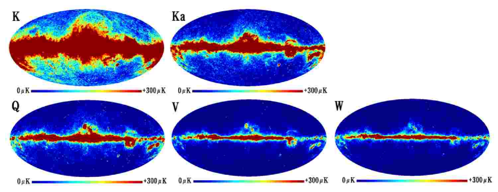
Figure 1.— The three-year version of Galactic foreground emission maps at five WMAP frequencies (K, Ka, Q, V, and W bands) made by co-adding synchrotron, free-free, and dust emission components derived from the MEM. The resolution of each map is $1\arcdeg$ FWHM. The Mollweide projection in Galactic coordinates is used to display all maps. In each figure, the Galactic center is located at the center and the Galactic plane lies at the horizontal line that passes through the Galactic center. Galactic longitude increases from center to left ($l=0\arcdeg$–$180\arcdeg$) and from right to center ($l=180\arcdeg$–$360\arcdeg$) while Galactic latitude increases from bottom to top ($b=-90\arcdeg$–$+90\arcdeg$).

2. Internal Linear Combination Method

2.1. ILC with a Minimum Variance Constraint

We find an optimal weight set for linear combination of observed CMB maps to remove the Galactic foregrounds with the constraint that the combined map have the minimum variance. Let us denote the observed temperature at $p$-th pixel and at $i$-th frequency band by $T_{i}(p)$. The observed temperature is a sum of the CMB temperature, instrument noise, and the Galactic emission. We perform ILC on a region $\mathcal{R}$ by minimizing the variance of the weighted sum of observed temperatures at pixels within the region. For multi-frequency CMB data with $k$ bands, the temperature of $p$-th pixel of the linearly combined map can be written as

$$T(p)=\sum_{i=1}^{k}w_{i}T_{i}(p)=\sum_{i=1}^{k-1}w_{i}D_{ik}(p)+T_{k}(p),$$ (3)

where $D_{ik}(p)\equiv T_{i}(p)-T_{k}(p)$ and $\sum_{i=1}^{k}w_{i}=1$. The variance of $T(p)$ over pixels within the region $\mathcal{R}$ is given by

$$\begin{split}\sigma^{2}&(T)={1\over N_{\mathcal{R}}}\sum_{p\in\mathcal{R}}\left[T(p)-\bar{T}\right]^{2}\\ &={1\over N_{\mathcal{R}}}\sum_{p\in\mathcal{R}}\left[\sum_{i=1}^{k-1}w_{i}\left\{D_{ik}(p)-\bar{D}_{ik}\right\}+\left\{T_{k}(p)-\bar{T}_{k}\right\}\right]^{2},\end{split}$$ (4)

where $\bar{T}$ represents the average of $T(p)$ over $N_{\mathcal{R}}$ pixels within the specified region $\mathcal{R}$. ILC coefficients that give the minimum variance is obtained by solving linear equations $\partial\sigma^{2}(T)/\partial w_{j}=0$, where $j=1,\cdots,k-1$. The solution $\mathbf{w}=(w_{1},\cdots,w_{k-1})^{T}$ is simply obtained from

$$\mathbf{w}=-\mathbf{S}^{-1}\mathbf{t}.$$ (5)

Here components of the $(k-1)\times(k-1)$ symmetric matrix $\mathbf{S}$ and the $(k-1)\times 1$ vector $\mathbf{t}$ are given by

$$\begin{split}&S_{ij}={1\over N_{\mathcal{R}}}\sum_{p\in\mathcal{R}}\left\{D_{ik}(p)-\bar{D}_{ik}\right\}\left\{D_{jk}(p)-\bar{D}_{jk}\right\},\\ &t_{j}={1\over N_{\mathcal{R}}}\sum_{p\in\mathcal{R}}\left\{T_{k}(p)-\bar{T}_{k}\right\}\left\{D_{jk}(p)-\bar{D}_{jk}\right\},\end{split}$$ (6)

where $i,j=1,\cdots,k-1$. The weight for the last frequency band map is $w_{k}=1-\sum_{i=1}^{k-1}w_{i}$. With the set of ILC weights, a foreground-reduced CMB map can be obtained from equation (3) (see $\S$3).

2.2. Defining Pixel-Groups with Common Foreground Spectral Properties

The efficiency of foreground reduction by the linear combination method becomes highest when the region contains pixels with the same foreground spectral variation over frequencies. On the other hand, if a region contains a large number of pixels whose Galactic foreground spectral property varies dramatically over the sky, as is the region $\mathcal{R}=0$ of WILC3YR (see Fig. 5$a$), the ILC just tries to find the best-fit combination weights that is optimal only to the average foreground spectral behavior. The ILC then results in positive or negative residual bias in the map ($\S\ref{subsec_applwmap}$).

To assess the Galactic foreground properties, we use the MEM Galactic foreground maps derived by the WMAP team, which are shown in Figure 1. The WMAP team has tried to distinguish different emission sources from one another by applying the MEM to the WMAP data, where the prior spatial distribution and spectral behavior of foreground components have been assumed by using the Galactic template maps. From this information the team has produced synchrotron, free-free, and dust emission maps with $1\arcdeg$ resolution at each WMAP frequency. For each band, we co-add three emission maps to make a Galaxy foreground map, upgrade its resolution to $\textrm{N}\textrm{side}=512$, and further smooth the map with a Gaussian filter with variable widths ($0\arcdeg$ – $2\arcdeg$) to reduce the MEM reconstruction noise. We smooth each Galaxy map over $\textrm{FWHM}=0\fdg 5$, and then subtract it from the unsmoothed Galaxy map to make a difference map, from which the standard deviation is calculated at the region with $|b|>60\arcdeg$. The signal-to-noise ratio at each pixel for each band is defined as the foreground intensity divided by the standard deviation. The minimum value among the five signal-to-noise ratios at each pixel is considered as the representative signal-to-noise ratio (S/N). The width of the smoothing filter has been set to zero for $\textrm{S/N}\geq 10$, and $\textrm{FWHM}=0.2(10-\textrm{S/N})$ for $\textrm{S/N}<10$.

Table 1 lists the spherical harmonic coefficients ($a_{lm}$) of the K-band Galactic foreground map up to $l=6$. The $a_{lm}$’s of foreground emissions at higher frequency bands have similar patterns with smaller amplitudes. The Galactic foreground emission is strong at even $l$-modes, among which $l=2$ and $m=0$ mode is the strongest one. The real components of even (odd) $m$-modes for even (odd) $l$ are stronger than the imaginary components. Modes of strong Galactic signal are expected to affect the corresponding modes of CMB signal significantly, resulting in biases in the reconstruction maps.

Table 1Low $l$-mode spherical harmonic coefficients of the K-band Galactic foreground emission

$l$	$m$	Re[$a_{lm}$]	Im[$a_{lm}$]	$l$	$m$	Re[$a_{lm}$]	Im[$a_{lm}$]
2	0	$-2153.7$	$0.0$	5	0	$1.6$	$0.0$
	1	$-140.0$	$36.6$		1	$-840.7$	$40.5$
	2	$412.5$	$172.6$		2	$2.2$	$-56.4$
3	0	$14.0$	$0.00$		3	$158.2$	$100.0$
	1	$875.4$	$-31.1$		4	$3.5$	$9.3$
	2	$3.1$	$41.4$		5	$-107.8$	$32.3$
	3	$-218.3$	$-115.8$	6	0	$-1672.5$	$0.0$
4	0	$1871.2$	$0.0$		1	$-98.1$	$100.1$
	1	$121.2$	$-97.2$		2	$187.2$	$120.3$
	2	$-244.5$	$-121.5$		3	$66.1$	$13.3$
	3	$-104.9$	$2.2$		4	$-208.8$	$13.5$
	4	$361.4$	$-46.1$		5	$-14.5$	$33.7$
					6	$-208.6$	$-121.5$

Note. — The coefficients are calculated in Galactic coordinates in units of $\mu\textrm{K}$.

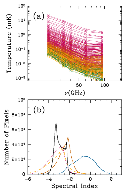
Figure 2.— ($a$) Intensity variation of the Galaxy foregrounds over WMAP frequencies ($22.8$ [K], $33.0$ [Ka], $40.7$ [Q], $60.8$ [V], and $93.5$ GHz [W]). According to levels of Galactic latitudes (low to high), plots are shown with different colors (red to blue). Only about 200 pixel values are shown to avoid overlaps. ($b$) Histograms of foreground spectral indices measured at K–Ka (dotted), Ka-Q (dashed), Q–V (long-dashed), and V–W (dot-dashed curve) frequency intervals. The solid curve denotes a histogram of spectral indices measured from four foreground intensities at K to V bands. The MEM Galactic foreground maps smoothed with a Gaussian filter of variable widths have been used for spectral index measurement.

Figure 2$a$ shows intensity variations of the Galactic foreground emission across WMAP bands at about 200 randomly selected pixels. Figure 2$b$ shows the histograms of foreground spectral indices ($\alpha$) within K–Ka, Ka–Q, Q–V, and V–W frequency intervals measured at all pixels in the sky. Each spectral index is measured by modeling the foreground intensity by $I_{\nu}\propto\nu^{\alpha}$. The spectral indices measured at frequency interval V–W (dot-dashed curve) have a wide range of values from negative to positive, centered at $\alpha\approx-0.6$ unlike those at K–Ka, Ka–Q, and Q–V that are located at $\alpha\lesssim-1$ (dotted, dashed, and long-dashed curves). Therefore, it is reasonable to treat spectral indices at low (K–V) and high (V–W) frequency intervals separately. For simplicity, we use an average spectral index measured for four foreground intensities from K to V bands as the representative spectral index at low frequency bands (Fig. 2$b$; solid curve). Hereafter we call the spectral indices measured at the low and high frequency intervals $\alpha$ and $\beta$, respectively.

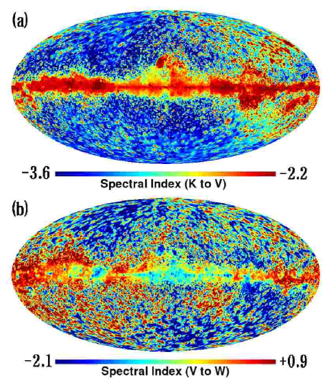
Figure 3.— All-sky maps showing distributions of foreground spectral indices measured at ($a$) low (K–V) and ($b$) high (V–W) frequency intervals. The MEM Galactic foreground maps smoothed with a Gaussian filter of variable widths have been used to measure the spectral indices.

Distributions of the spectral indices on the sky measured at low and high frequency intervals are shown in Figure 3. The Galactic plane region has spectral indices of $\alpha\approx-2.5$ – $-2.0$ and $\beta\approx-1.0$ – $+1.0$ while the high latitude region with low foreground contamination shows large fluctuations, especially for $\beta$ map. It should be noted that the spectral index is a sensitive function of both frequency and direction, and that the foreground subtraction of ILC will be most successful when the ILC is performed at a region where the foreground characteristic is most homogeneous.

For each of the two histograms of spectral indices at the high and low frequency bands (Fig. 2$b$), we define twenty spectral index bins so that each bin contains equal number ($157,300$) of pixels with similar foreground spectral properties. By combining the two sets of spectral-index bins, one at low and the other at high frequency band, we define four hundred ($20\times 20=400$) groups of pixels with similar spectral indices. Because pixels within the same $\alpha$-bin have a wide range of spectral index $\beta$, the number of pixels contained in each group differs from group to group. The resulting group index map is shown in Figure 4$a$. The variation of the spectral index across the sky is naturally taken into account in this way. We note that pixels at the high latitude regions are assigned with a wide range of group indices. The ILC will be applied separately for each group of pixels with similar foreground spectral properties to obtain foreground-reduced CMB temperatures in the next section.

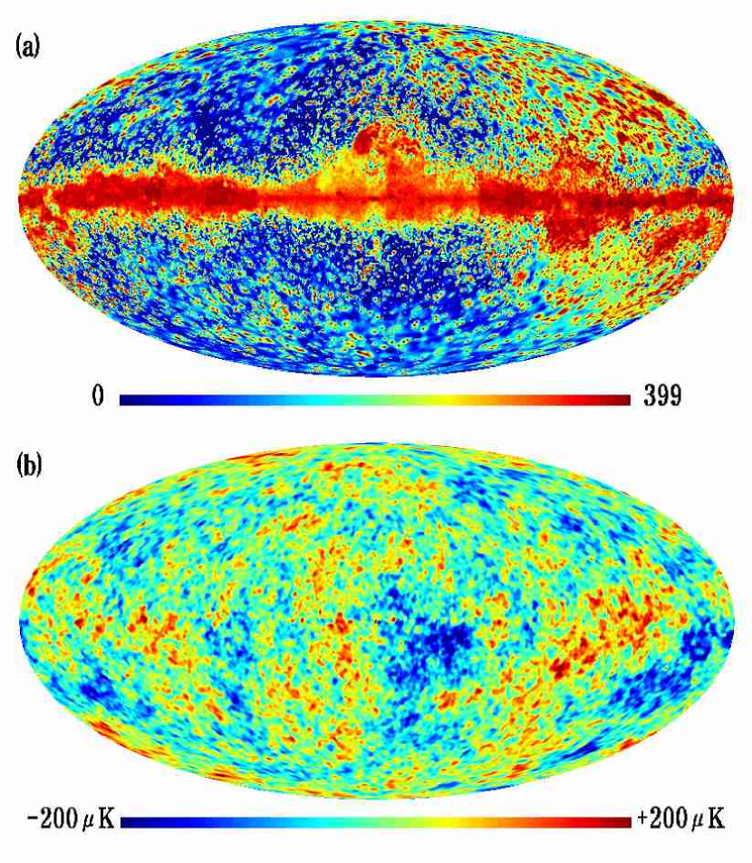
Figure 4.— ($a$) A group index map showing four hundred groups of pixels with similar foreground properties defined by using the foreground spectral index maps at low and high frequency bands (Fig. 3). The group index runs from $0$ to $399$. ($b$) The foreground-reduced CMB temperature fluctuation map (SILC400) derived from the five-band WMAP maps by applying the ILC method which adopts the pixel-groups as defined in ($a$). The SILC400 has been corrected for the residual bias, and the monopole and dipole have been removed from the map. Due to the further smoothing with a Gaussian filter of $\textrm{FWHM}=1\arcdeg$, the map resolution is $1\fdg 414$ FWHM. The SILC400 is available at http://newton.kias.re.kr/~parkc/CMB/SILC400.html together with its spherical harmonic coefficients $a_{lm}$ up to $l=200$.

3. Application to the WMAP Three-Year data

3.1. The ILC Map Derived From the WMAP Three-Year Maps: SILC400

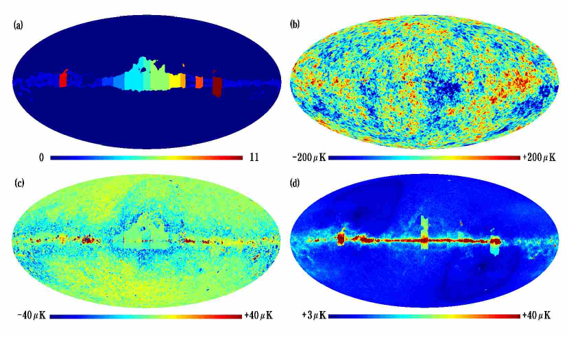
Figure 5.— ($a$) Region definition map defined by the WMAP team (12 regions). ($b$) A foreground-reduced CMB map derived with the minimum-variance ILC method (WILC12). The ILC has been applied to 12 regions independently. Maps showing ($c$) the average and ($d$) the standard deviation of the residual foreground emissions in the ILC map estimated from two hundred WILC12 simulation maps. The monopole and dipole components of the average map have been removed.

We apply our ILC method to the WMAP three-year data. The WMAP has one K band ($22.8$ GHz), one Ka band ($33.0$ GHz), two Q band ($40.7$ GHz), two V band ($60.8$ GHz), and four W band ($93.5$ GHz) differencing assemblies, with $0\fdg 82$, $0\fdg 62$, $0\fdg 49$, $0\fdg 33$, and $0\fdg 21$ FWHM beam widths, respectively. The WMAP maps are made in the HEALPix format with $\textrm{Nside}=512$ (Górski et al., 1999, 2005). The total number of pixels of a map is $12\times\textrm{Nside}^{2}=3,145,728$.

We use the five band-averaged WMAP maps with $1\arcdeg$ FWHM resolution that are presented by the WMAP team. The maps have been produced in the following way. Each map of each differencing assembly is deconvolved with the corresponding channel-specific beam and convolved with $\textrm{FWHM}=1\arcdeg$ beam. The maps of the same frequency band are averaged with noise-weight at each pixel taken into account, and finally the five WMAP maps at K, Ka, Q, V, and W bands with $\textrm{FWHM}=1\arcdeg$ resolution are obtained.

We obtain a foreground-reduced ILC map (hereafter WILC12) from the three-year WMAP data with $1\arcdeg$ FWHM resolution at five frequency bands ($k=5$) by using equations (3), (5) and (6) for each of 12 disjoint regions that are defined by the WMAP team (Figs. 5$a$ and $b$). Our weight coefficients are slightly different from those found by Hinshaw et al. (2006) who compute minimum-variance ILC weights by using Lagrange multipliers, but our weight sets give smaller variances. To estimate the residual bias in the WILC12 map we generate two hundred maps mimicking the WILC12 map by combining theoretical CMB temperature signal with instrument noise and foreground emissions. The three-year version of MEM Galactic foreground maps have been used as the contaminating sources. The average and the standard deviation maps of residual emission in two hundred WILC12 simulation maps with respect to the true CMB temperatures are shown in Figures 5$c$ and $d$. From the WILC12 simulations, we found that ILC applied to the large high latitude region that contains pixels with a wide range of foreground spectral indices (e.g., the region with index $\mathcal{R}=0$) induces residual biases whose levels are different at different positions on the sky. As shown in Figure 5$c$, the residual emission is negative near the Galactic plane and is positive at high latitude region.

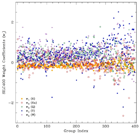
Figure 6.— Minimum-variance ILC weights of SILC400 obtained for four hundred pixel-groups. The ILC weights are denoted as yellow filled circles for K ($w_{1}$), red open circles for Ka ($w_{2}$), green open squares for Q ($w_{3}$), blue filled squares for V ($w_{4}$), and violet crosses for W ($w_{4}$) bands.

Figure 4$b$ shows a new foreground-reduced CMB map obtained by applying the ILC method described in $\S\ref{sec_ilcmethod}$ with the minimum variance constraint, where the combinations are performed for four hundred pixel-groups of common spectral properties independently (hereafter SILC400). The SILC400 shown here is a map that has been corrected for the residual bias based on the ILC simulation as described in $\S\ref{ILC:sim}$, and the monopole and dipole have been subtracted from the map. The map has been shown after further smoothed by a Gaussian filter of $\textrm{FWHM}=1\arcdeg$ to reduce discontinuities between boundaries of pixel groups. In the subsequent analysis of large scale modes, however, we use the unsmoothed SILC400.

ILC combination weights for 400 groups are plotted in Figure 6. The combination weights varies dramatically from group to group, except for the K-band weights ($w_{1}$; filled circles) that are stably distributed around $-0.25$. Most of the weights in Ka–W bands ($w_{2}$–$w_{5}$) are positive for group index $\lesssim 250$ corresponding to high latitude regions, while they are fluctuating at the Galactic plane regions (group index $\gtrsim 250$).

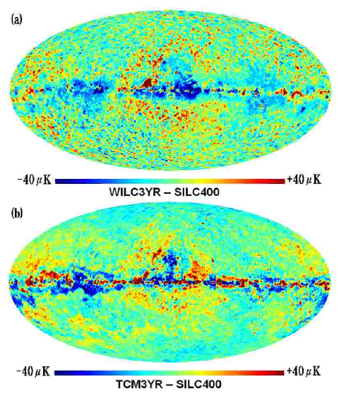
Figure 7.— Comparison of SILC400 with other foreground-reduced CMB maps ($a$) WILC3YR and ($b$) TCM3YR. Shown are differences of WILC3YR and TCM3YR from SILC400. Before differencing, all maps are prepared to have $\textrm{FWHM}=1\fdg 414$ resolution and the monopole and dipole modes are removed.

Comparisons of SILC400 with other foreground-reduced maps (WILC3YR and TCM3YR) are shown as difference maps in Figure 7, where all maps are made to have $1\fdg 414$ FWHM resolution with the monopole and the dipole components removed before differencing. The WILC3YR is similar to SILC400 within $40~{}\mu\textrm{K}$ difference, except for the Galaxy center and cirrus regions. The cirrus is apparent as red and the Galactic center looks partly blue. For TCM3YR, its difference from SILC400 shows the region boundaries near the Galactic plane and mid-latitude, especially at $l=0\arcdeg$ – $180\arcdeg$ (left part in Fig. 7$b$), where positive and negative temperatures appear interchangeably. Those region boundaries were defined by Tegmark et al. (2003).

Table 2Low $l$-mode spherical harmonic coefficients of the Minimum-Variance ILC Map SILC400

$l$	$m$	Re[$a_{lm}$]	Im[$a_{lm}$]	$l$	$m$	Re[$a_{lm}$]	Im[$a_{lm}$]
2	0	$7.51$	$0.00$	5	0	$14.33$	$0.00$
	1	$-1.54$	$4.82$		1	$23.96$	$1.09$
	2	$-18.54$	$-18.01$		2	$-7.75$	$2.78$
3	0	$-5.25$	$0.00$		3	$19.75$	$3.58$
	1	$-10.74$	$3.76$		4	$-4.21$	$8.53$
	2	$22.54$	$2.13$		5	$9.48$	$20.26$
	3	$-13.52$	$30.10$	6	0	$-1.76$	$0.00$
4	0	$23.31$	$0.00$		1	$0.78$	$4.17$
	1	$-6.97$	$9.12$		2	$10.39$	$-2.75$
	2	$11.14$	$4.26$		3	$-9.02$	$-0.28$
	3	$7.34$	$-21.02$		4	$13.73$	$-1.56$
	4	$1.75$	$-9.68$		5	$-5.07$	$-3.74$
					6	$3.64$	$8.91$

Note. — The coefficients are calculated in Galactic coordinates in units of $\mu\textrm{K}$. The $l=2$ coefficients for WILC3YR are $a_{20}=11.48$, $a_{21}=-0.05+4.86i$, and $a_{22}=-14.41-18.80i$. For TCM3YR, $a_{20}=3.34$, $a_{21}=0.26+4.88i$, and $a_{22}=-14.88-17.26i$.

Low $l$-mode spherical harmonic coefficients ($a_{lm}$) of SILC400 are listed in Table 2 ($l=2$ coefficients for WILC3YR and TCM3YR are summarized in the note). We note that the SILC400 has $a_{20}$ ($=7.51~{}\mu\textrm{K}$) that is between those of TCM3YR ($3.34~{}\mu\textrm{K}$) and WILC3YR ($11.5~{}\mu\textrm{K}$), and also has slightly different $a_{22}$. The amplitudes of $a_{20}$ and $a_{22}$ are bigger than $a_{21}$ both in SILC400 and the Galactic foreground map (Table 1). However, $a_{20}$ and $a_{22}$ have different signs in two maps: the quadrupole of CMB and the Galaxy are negatively correlated (see $\S\ref{sec_discuss}$). This is mainly due to the big cold spot in the CMB map at the Galactic center region (see Fig. 4).

3.2. Simulations: Test for the ILC Method

As shown in $\S\ref{subsec_applwmap}$, SILC400 differs from foreground-reduced CMB maps previously made by others. Because the ILC method conserves the blackbody nature of the CMB signal, all maps contain exactly the same information for CMB temperature fluctuations but with different level of foreground residuals. To quantify the level of the residual foreground in our variance-minimized ILC map, we have performed two hundred simulations that mimic the WMAP data and analyzed them in the same way that SILC400 is made.

First, we simulate two hundred WMAP Gaussian CMB signal maps for each differencing assembly at each band. The concordance flat $\Lambda\textrm{CDM}$ model power spectrum that fits to the WMAP data only, has been used (Spergel et al., 2006). For each mock observation, the same $a_{lm}$’s are used for all frequency channels. During the map generation, the WMAP beam transfer function $B_{l}$ is used for each differencing assembly, and the instrument noise at each pixel is randomly drawn from the Gaussian distribution with variance of $\sigma_{0}^{2}/N_{\textrm{obs}}$, where $N_{\textrm{obs}}$ is the effective number of observations at each pixel, and $\sigma_{0}$ is the global noise level of the map (Table 1 of Hinshaw et al. 2006).

Secondly, for each differencing assembly realization, we deconvolve the beam effect, and convolve the map to a common resolution of $1\arcdeg$ Gaussian FWHM. Differencing assembly maps at the same band are averaged with weights given by the noise variance at each pixel to produce an average map at each frequency band. Finally, the Galactic foreground map (with $1\arcdeg$ FWHM resolution) at each frequency is co-added to the average WMAP CMB map. We do not use the Galactic template method to mimic the Galactic foreground emissions as used in Eriksen et al. (2004a), but use the Galactic foreground maps derived by MEM from the three-year WMAP data. Compared to weighted average of template maps, these foreground maps reasonably describe the Galactic foreground emission even at the Galactic plane. However, the Galactic foreground maps derived by the MEM are somewhat noisy because of the MEM reconstruction noise. For each simulation, the five foreground-added CMB maps are put into the same ILC pipeline as used in $\S\ref{subsec_applwmap}$.

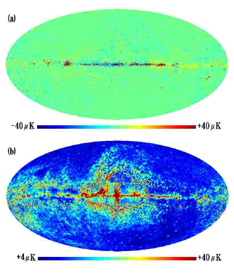
Figure 8.— ($a$) Average and ($b$) standard deviation maps of the residual foreground emissions with respect to true CMB temperatures in two hundred SILC400 simulation maps.

Figure 8 shows average and standard deviation maps of the residual foreground emissions with respect to true CMB temperatures in two hundred SILC400 simulation maps. It demonstrates that except for the Galactic plane region our ILC method correctly reconstructs the CMB signal without significant bias due to the Galactic foreground contamination unlike the average residual-emission map of WILC12 simulations (Fig. 5$c$). However, some residual foreground features with $10$–$30~{}\mu\textrm{K}$ levels are seen at the high Galactic latitude regions, where the foreground emission is very weak at high frequency bands (V and W) and the spectral index $\beta$ has been measured with large uncertainty due to the MEM reconstruction noises (upper right part of Fig. 8$a$). The standard deviation map indicates that SILC400 may be contaminated by the residual foreground at the Galactic plane and the mid-latitude regions. Compared with the WILC12 case (Fig. 5$d$), the standard deviation map has larger amplitudes at high latitude region, because pixel-groups used for SILC400 contain much fewer pixels than the $\mathcal{R}=0$ region of WILC12.

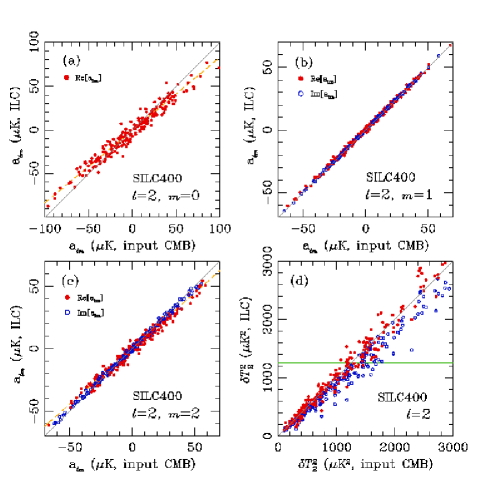
Figure 9.— ($a$)–($c$) Plots of $l=2$ spherical harmonic coefficients ($a_{lm}$) calculated from two hundred SILC400 simulation maps against those from true CMB maps (filled circles for real and the open circles for imaginary components). For real components of even $m$ modes, each plot has been fitted with a straight line (dashed lines). ($d$) Plot of quadrupole powers measured from SILC400 simulation maps against those from the true CMB maps (open circles). Quadrupole powers measured from bias-corrected $a_{lm}$’s of SILC400 simulations maps are plotted against the true values as filled circles.

Figures 9$a$, $b$, and $c$ compare the spherical harmonic coefficients of $l=2$ mode calculated from two hundred SILC400 simulation maps with those of true input CMB maps. To reduce the effect of the residual bias, we have subtracted the average map of the residual foreground emission from each SILC400 simulation map before calculating the $a_{lm}$. The $a_{20}$ and the real component of $a_{22}$ are contaminated by the residual Galactic emission in the sense that each plot, when fitted with a straight line (dashed lines), gives a slope less than $1$, and some scatter is seen in the $a_{20}$ plot. Quadrupole powers from two hundred SILC400 simulations against true CMB quadrupole powers are shown as open circles in Figure 9$d$, where the quadrupole power predicted in the concordance $\Lambda\textrm{CDM}$ model is denoted as horizontal line ($\delta T_{2}^{2}=1250$ $\mu\textrm{K}^{2}$; Spergel et al. 2006). The SILC400 systematically underestimates the CMB quadrupole powers, but with much less scatter than LILC simulations (see Fig. 6 of Eriksen et al. 2004a).

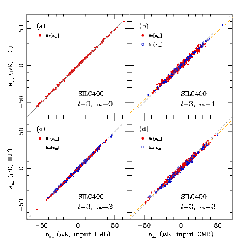
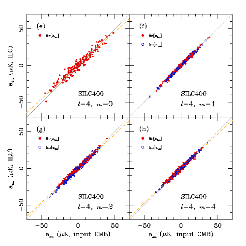
Figure 10.— Plots of spherical harmonic coefficients ($a_{lm}$’s) estimated from two hundred SILC400 simulation maps against those from true CMB maps for ($a$)–($d$) $l=3$ and ($e$)–($h$) $l=4$ modes. The $a_{43}$ plot is omitted because it is very similar to $a_{41}$ plot.

Spherical harmonic coefficients for $l=3$ and $4$ of SILC400 simulations are compared with true values in Figure 10. The $l=3$ modes are excellently reconstructed in the SILC400 simulations, although plots for real components of $a_{31}$ and $a_{33}$ against true values show slight decrease in correlation slopes. For $l=4$, the real components of $a_{40}$ and $a_{42}$ show similar patterns to $l=2$ case. The residual foreground emission has induced slope decrease and scatter in the $a_{40}$ plot (Fig. 10$e$).

We can remove the systematic effects of the ILC foreground reduction method on $a_{lm}$ of the SILC400 simulation maps. We have estimated the true $a_{lm}$ up to $l=200$ by applying a simple relation $a_{lm}=(a_{lm}^{\textrm{ILC}}-b)/a$, where $a_{lm}^{\textrm{ILC}}$ is the spherical harmonic coefficient obtained from each SILC400 simulation map from which the average residual bias map of Figure 8$a$ has been subtracted, and $a$ and $b$ denote a correlation slope and an offset from the line-fit. Linear fit parameters have been derived from the $a_{lm}$ plots, where each slope and offset are obtained for real or imaginary components of $a_{lm}$’s, independently. Real components of $a_{lm}$ for even (odd) $l$ and even (odd) $m$ modes show the systematic decreases in the slope of the linear relation. However, in all cases, no large offset is observed in the SILC400 simulations. The result for $l=2$ is shown as filled circles in Figure 9$d$. The quadrupole powers of SILC400 simulation maps, which were underestimated before correction, now have the correct mean amplitudes compared with the true values. Figure 11 shows the low $l$-mode powers of SILC400 simulations versus true CMB powers for $l=3$–$6$ before (open circles) and after (filled circles) the bias correction for $a_{lm}$.

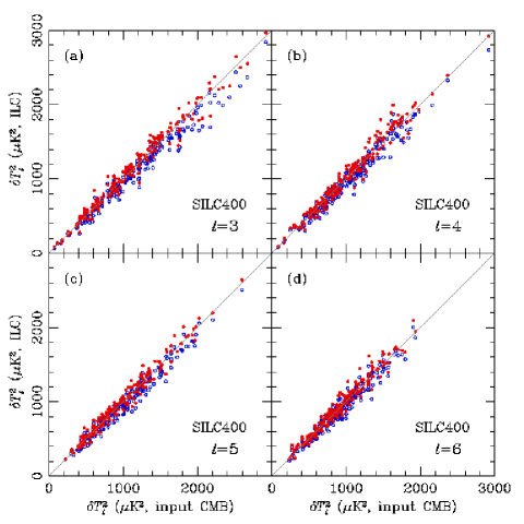
Figure 11.— ($a$)–($d$) Plots of low $l$-mode powers ($l=3$–$6$) estimated from two hundred SILC400 simulation maps against those from true CMB maps before (open circles) and after (filled circles) the effect of bias due to the residual Galactic emission on $a_{lm}$’s is removed.

4. Statistics of Large-Scale Modes

Table 3CMB quadrupole and octopole powers

Measurement	$\delta T_{2}^{2}$ ($\mu\textrm{K}^{2}$)	$p$ value	$\delta T_{3}^{2}$ ($\mu\textrm{K}^{2}$)
Spergel et al. best-fit $\Lambda$CDM model	$1250$	$\cdots$	$1143$
Hinshaw et al. cut sky analysis	$211.0$	2.6%	$1041$
WMAP team’s ILC map (WILC3YR)	$248.5$	3.7%	$1051$
Tegmark et al. cleaned map (TCM)	$201.6$	2.3%	$866.1$
de Oliveira-Costa & Tegmark cleaned map (TCM3YR)	$209.6$	2.5%	$1037.8$
Eriksen et al. ILC map (LILC)	$350.6$	7.6%	$1090$
Minimum-variance ILC map (SILC400)	$244.5_{-203.3}^{+83.8}$	4.9%†	$859.4_{-109.0}^{+61.2}$
SILC400 (bias corrected)	$275.8_{-126.0}^{+94.3}$	5.7%†	$951.9_{-83.0}^{+63.7}$

Note. — $p$ value denotes the probability of finding a lower quadrupole than the measured value if the concordance $\Lambda$CDM model (Spergel et al., 2006) is correct. The $p$ values with $\dagger$ have been estimated from equation (7).

Table 3 summarizes the quadrupole and octopole powers measured from the WMAP data in the previous studies, including our new estimates. For SILC400 results, the 68% confidence limits have been deduced from the distribution of $\delta T_{l}^{2}(\textrm{ILC})-\delta T_{l}^{2}(\textrm{CMB})$ in two hundred SILC400 simulations. The third column of Table 3 lists the probabilities ($p$) of the quadrupole power being as low as measured value if the concordance $\Lambda$CDM model is correct (de Oliveira-Costa et al., 2004). However, the $p$ values for SILC400 maps have been estimated from

$$\hat{p}=\int dQ_{\textrm{obs}}p(Q<Q_{\textrm{obs}})p(Q_{\textrm{obs}}),$$ (7)

where $Q$ denotes quadrupole power and $p(Q<Q_{\textrm{obs}})$ is the probability of finding the quadrupole power as low as the observed value $Q_{\textrm{obs}}$. The $p(Q_{\textrm{obs}})$ is the probability of observing the quadrupole power $Q_{\textrm{obs}}$ and is calculated from the distribution of quadrupole powers from two hundred SILC400 simulations. The quadrupole power of SILC400 ($244.5_{-203.3}^{+83.8}~{}\mu\textrm{K}^{2}$) is close to that of WILC3YR ($248.5~{}\mu\textrm{K}^{2}$) and is between values of TCM3YR ($209.6~{}\mu\textrm{K}^{2}$) and LILC ($350.6~{}\mu\textrm{K}^{2}$). Our estimates compare with those of Bielewicz et al. (2004) who have applied power equalization filter to the high latitude WMAP data and obtained $\delta T_{2}^{2}=279\pm 49$ and $\delta T_{3}^{2}=870\pm 98$ from TCM.

Also listed in Table 3 are the quadrupole and octopole powers from SILC400 after removing the expected biases in $a_{lm}$ due to the minimum variance ILC method. Our bias-corrected quadrupole power ($275.8_{-126.0}^{+94.3}~{}\mu\textrm{K}^{2}$) is higher than the WMAP team’s measurement (Hinshaw et al., 2006), but they are still consistent with each other. The probability of observing such a low quadrupole power in the concordance $\Lambda\textrm{CDM}$ universe is as high as $p=5.7\%$.

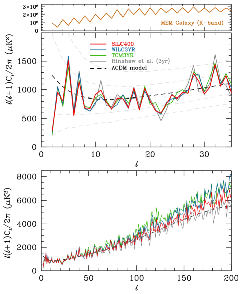
Figure 12.— Power spectra measured from SILC400 (thick red), WILC3YR (blue), and TCM3YR (green curve). The power spectrum of K-band MEM Galactic foreground map has also been shown for comparison (brown curve). Beam effects are deconvolved for the correct amplitudes of power spectra. The WMAP power spectrum measured by Hinshaw et al. (2006) (grey curve), and the $\Lambda\textrm{CDM}$ model of Spergel et al. (2006) (dashed curve) are shown for comparison with 68% and 95% confidence limits (grey dashed curves).

Figure 12 compares SILC400 power spectrum with other measurements up to $l=35$ (top) and $l=200$ (bottom). Also shown in the top panel is the power spectrum of K-band MEM Galactic foreground map whose zigzag pattern at $l=2$–$8$ is very similar to that of the CMB power spectra. For WILC3YR, TCM3YR, and SILC400, we have deconvolved the beam effects to obtain correct amplitudes of power spectrum. The WMAP team’s power spectrum measurement from the cut-sky analysis and the best-fit $\Lambda\textrm{CDM}$ power spectrum are also shown for comparison with 68% and 95% confidence limits (Hinshaw et al., 2006; Spergel et al., 2006). The quadrupole power of the $\Lambda$CDM model is $1250~{}\mu\textrm{K}^{2}$ with 68% and 95% confidence intervals, $510$–$1961~{}\mu\textrm{K}^{2}$ and $198$–$3311~{}\mu\textrm{K}^{2}$, respectively (from the ten thousand realizations).

Our new estimate of power spectrum from SILC400 (red curve) is very similar to others up to $l\approx 30$. Due to the instrument and reconstruction noises, all ILC maps give angular power spectra with higher amplitudes with increasing $l$, compared with the $\Lambda$CDM model. As shown in Figure 12 (bottom), the angular power spectrum of the SILC400 has lower amplitude than those of WILC3YR and TCM3YR up to $l=200$, which indicates that our ILC method better satisfies the minimum variance constraint.

It has been reported that both the quadrupole and the octopole of the WMAP map appear planar, with most of their hot and cold spots located on a single plane in the sky, and the two planes appear roughly aligned (de Oliveira-Costa et al., 2004). A simple way to quantify a preferred axis for arbitrary multipoles is to find the axis $\hat{\mbox{\boldmath$n$}}$ around which the angular momentum dispersion

$$\left<\psi|(\hat{\mbox{\boldmath$n$}}\cdot{\bf L})^{2}|\psi\right>=\sum_{m}m^{2}|a_{lm}(\hat{\mbox{\boldmath$n$}})|^{2}$$ (8)

is maximized (de Oliveira-Costa et al., 2004), where the CMB map is considered as a wave function $\Delta T(\hat{\mbox{\boldmath$n$}})\equiv\psi(\hat{\mbox{\boldmath$n$}})$. Here $a_{lm}(\hat{\mbox{\boldmath$n$}})$ denotes the spherical harmonic coefficients of the CMB map in a rotated coordinate system with its $z$-axis in the $\hat{\mbox{\boldmath$n$}}$ direction. For each $l$ we find a unit vector $(\hat{\mbox{\boldmath$n$}}_{l})$ that maximizes the angular momentum dispersion. We start to evaluate equation (8) for all the unit vectors corresponding to HEALPix pixel centers at resolution $\textrm{Nside}=32$, perform the same operation only for pixels at higher resolution around the unit vector found in the previous step, and finally obtain a unit vector that maximizes equation (8) at resolution $\textrm{Nside}=4096$.

Table 4 lists directions of the quadrupole and the octopole and separations between two poles measured from the WMAP data. The 68% confidence limits for the measured angular separation $\theta_{23}$ of SILC400 have been estimated from the distribution of $\theta_{23}(\textrm{ILC})-\theta_{23}(\textrm{CMB})$ in two hundred SILC400 simulations. Since the quantity $|\hat{\mbox{\boldmath$n$}}_{2}\cdot\hat{\mbox{\boldmath$n$}}_{3}|$ has a uniform distribution on the unit interval $\left[0,1\right]$, the probability of finding an angular separation smaller than the measured separation is simply given by $p=1-|\hat{\mbox{\boldmath$n$}}_{2}\cdot\hat{\mbox{\boldmath$n$}}_{3}|$ (last column in Table 4). However, the $p$ values for SILC400 maps have been calculated from equation (7) with $Q$ replaced with $\theta_{23}$. The bias-corrected SILC400 has an angular separation ($\theta_{23}=11\fdg 8_{-8\fdg 0}^{+6\fdg 4}$) that is somewhat larger than those from TCM, LILC, and WILC3YR but is very similar to that of TCM3YR. We find that the octopole directions ($\hat{\mbox{\boldmath$n$}}_{3}$) are more stable than the quadrupole directions ($\hat{\mbox{\boldmath$n$}}_{2}$). Our result for SILC400 confirms the previous results that the quadrupole and octopole directions are aligned (Tegmark et al. 2003; Eriksen et al. 2004a; Bielewicz et al. 2004; Copi et al. 2004, 2006; Schwarz et al. 2004), with $p=4.3$%.

Table 4Directions of the Quadrupole and the Octopole

Maps	$l_{2}$	$b_{2}$	$l_{3}$	$b_{3}$	$\theta_{23}$	$p$ value
WMAP team’s ILC map (WILC3YR)	$235\fdg 23$	$68\fdg 42$	$236\fdg 94$	$62\fdg 61$	$5\fdg 85$	0.52%
Tegmark et al. clean map (TCM)	$257\fdg 58$	$58\fdg 82$	$238\fdg 37$	$62\fdg 04$	$9\fdg 96$	1.51%
TCM3YR (de Oliveira-Costa & Tegmark 2006)	$224\fdg 04$	$76\fdg 56$	$236\fdg 75$	$63\fdg 98$	$13\fdg 23$	2.65%
Eriksen et al. ILC map (LILC)	$247\fdg 52$	$61\fdg 90$	$232\fdg 84$	$63\fdg 41$	$6\fdg 89$	0.72%
Minimum-variance ILC map (SILC400)	$240\fdg 78$	$75\fdg 24$	$234\fdg 47$	$62\fdg 26$	$13\fdg 16_{-6\fdg 79}^{+7\fdg 62}$	5.36%†
SILC400 (bias corrected)	$245\fdg 54$	$74\fdg 38$	$234\fdg 58$	$63\fdg 25$	$11\fdg 77_{-8\fdg 03}^{+6\fdg 40}$	4.29%†

Note. — $\theta_{23}$ is the angular separation defined as $\theta_{23}=\cos^{-1}(\hat{\mbox{\boldmath$n$}}_{2}\cdot\hat{\mbox{\boldmath$n$}}_{3})$, where $\hat{\mbox{\boldmath$n$}}_{2}=(l_{2},b_{2})$ and $\hat{\mbox{\boldmath$n$}}_{3}=(l_{3},b_{3})$. The $p$ values with $\dagger$ have been estimated from equation (7) with $Q$ replaced by $\theta_{23}$.

Figure 13 compares angular separations between quadrupole and octopole directions of two hundred SILC400 simulation maps with the true values, and demonstrates that SILC400 can reconstruct the correct multipole directions of low $l$-modes.

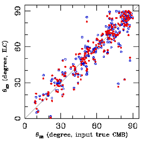
Figure 13.— Plots of angular separation ($\theta_{23}$) between the quadrupole and the octopole directions measured from two hundred SILC400 simulation maps against those from true CMB maps, before (open circles) and after (filled circles) the bias correction.

We also measure the degree of planarity of low $l$ modes by calculating the $t$ statistic defined by de Oliveira-Costa et al. (2004) as

$$t=\max_{\hat{\mbox{\boldmath$n$}}}{{|a_{l-l}|^{2}+|a_{ll}|^{2}}\over{\sum_{m=-l}^{+l}|a_{lm}|^{2}}}.$$ (9)

The $t$ statistic measures the maximal percentage of $l$-mode power that contributes to $|m|=l$, and we obtain $t$ value for each $l$ by finding a direction $\hat{\mbox{\boldmath$n$}}$ that maximizes equation (9). The maximization is performed over pixels of a map in the similar way as used in finding the quadrupole and octopole directions. The performance of our ILC method in reconstructing the true $t$-statistic is shown in Figure 14, where $t$ values of SILC400 simulation maps against those from true CMB maps are plotted for $l=2$–$6$ modes.

The $t$ values measured from the foreground-cleaned maps are summarized in Table 5. Numbers in the parentheses represent the number of occurrences that have larger $t$ values than the measured value among the two hundred SILC400 simulations. The 68% confidence limits for $l=2$ and $3$ are obtained from the distributions of $t(\textrm{ILC})-t(\textrm{CMB})$ in the SILC400 simulations. The $t$ value for $l=3$ mode of SILC400 (bias corrected; $t=0.91_{-0.03}^{+0.02}$) is very similar to the previously measured values, and implies that the octopole has high planarity. However, the planarity is not statistically significant because the probability that SILC400 simulation map has $t$ value larger than the measured $t$ value is 18.5%: thirty seven among two hundred SILC400 simulations. The probability of having the $t$ value for the quadrupole mode as high as the measured value of SILC400 ($t=0.98_{-0.02}^{+0.02}$) is still higher (98/200). As shown in Figure 14, most of the CMB quadrupole modes have $t>0.8$.

Table 5$t$ Values of Low Spherical Harmonic Modes

Maps	$l=2$	$l=3$	$l=4$	$l=5$	$l=6$
WMAP team’s ILC map (WILC3YR)	$0.930$	$0.917$	$0.648$	$0.375$	$0.798$
Tegmark et al. clean map (TCM)	$0.957$	$0.942$	$0.588$	$0.372$	$0.783$
TCM3YR (de Oliveira-Costa & Tegmark 2006)	$0.995$	$0.877$	$0.679$	$0.358$	$0.749$
Eriksen et al. ILC map (LILC)	$0.913$	$0.934$	$0.587$	$0.374$	$0.806$
Minimum-variance ILC map (SILC400)	$0.991_{-0.021}^{+0.017}$ (61)	$0.901_{-0.027}^{+0.029}$ (38)	$0.523$ (180)	$0.377$ (199)	$0.835$ (3)
SILC400 (bias corrected)	$0.977_{-0.024}^{+0.016}$ (98)	$0.908_{-0.028}^{+0.024}$ (37)	$0.530$ (177)	$0.382$ (199)	$0.826$ (4)

Note. — Numbers in the parentheses represent the number of occurrences that give larger $t$ values than the measured value among the two hundred SILC400 simulations.

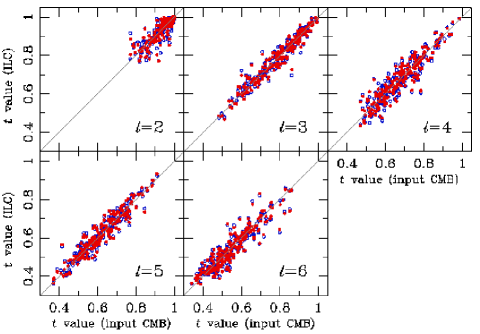
Figure 14.— Plots of $t$-statistic for $l=2$–$6$ modes measured from two hundred SILC400 simulation maps against those from true CMB maps, before (open circles) and after (filled circles) the bias correction.

As pointed by Eriksen et al. (2004a), the $l=5$ and $l=6$ modes are very peculiar in their symmetry properties. Only one case out of the two hundred SILC400 simulations has $t$ values larger than $t=0.38$ for $l=5$, and only four have $t$ values larger than $t=0.83$ for $l=6$, which indicates that the distribution of temperature fluctuation of $l=5$ mode is highly symmetric, and the $l=6$ mode is planar together with the $l=2$ and $l=3$ modes.

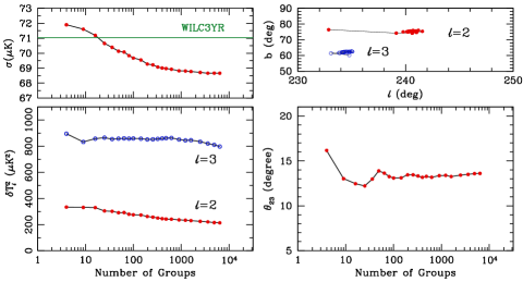
Figure 15.— Standard deviations ($\sigma$; top-left), the quadrupole and the octopole powers ($\delta T_{l}^{2}$; bottom-left), and angular separations between the quadrupole and the octopole ($\theta_{23}$; bottom-right panel) measured from ILC maps made for various number of pixel-groups from $4$ to $6400$. The top-right panel shows the variation of the quadrupole (filled circles) and the octopole (open circles) directions in Galactic coordinates. The horizontal line in the top-left panel denotes the standard deviation of the WILC3YR map.

We also investigate whether the measured statistics depend on the number of pixel-groups and the smoothing scale. First, we measure standard deviation, quadrupole and octopole powers, and angular separation between the two multipoles from the ILC maps made by fixing the resolution to $1\arcdeg~{}\textrm{FWHM}$ while varying the number of pixel-groups in the group-index map from $4$ ($2\times 2$) to $6400$ ($80\times 80$). The result is shown in Figure 15. The standard deviation and quadrupole power decrease with increasing number of pixel-groups, while the octopole power is very stable. If the number of pixel-groups is larger than $100$, all statistical quantities become stable. However, when the number of pixel-groups is small, a wide range of foreground spectral indices is allowed in a common group, and the ILC results in higher values of standard deviation, quadrupole power, and larger angular separation $\theta_{23}$. We note that $\theta_{23}$ becomes large because the quadrupole direction is unstable in this case (filled circles in the top-right panel of Fig. 15).

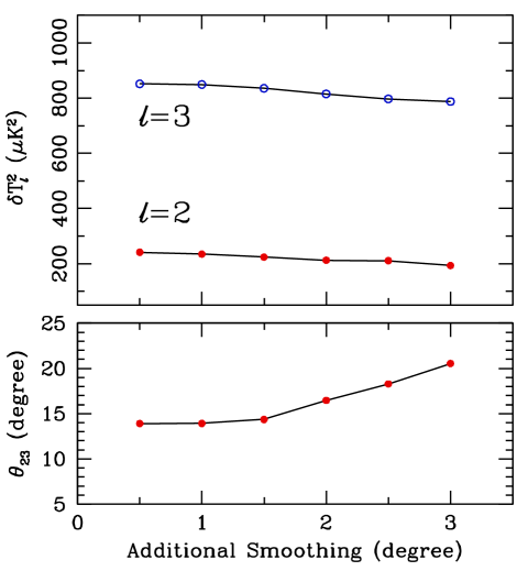
Figure 16.— Quadrupole and octopole powers ($\delta T_{l}^{2}$) and angular separations between the quadrupole and the octopole ($\theta_{23}$) measured from the ILC maps produced from the WMAP data and the Galactic foreground maps with various angular resolution. Each WMAP or Galaxy map with $\textrm{FWHM}=1\arcdeg$ has been further smoothed with a smoothing filter of $0\fdg 5$ to $3\fdg 0$ FWHM with steps of $0\fdg 5$. Total resolution of ILC maps varies from $1\fdg 12$ to $3\fdg 16$ FWHM.

Secondly, we measure the large scale mode statistics from the ILC maps produced from the WMAP data and the Galactic foreground maps with various angular resolution. Each WMAP map or MEM-derived Galactic foreground map, which has originally $1\arcdeg$ FWHM resolution, has been further smoothed with a Gaussian filter of $\textrm{FWHM}=0\fdg 5$–$3\fdg 0$ with steps of $0\fdg 5$ (the total resolution varies from $1\fdg 12$ to $3\fdg 16$ FWHM). The smoothed maps are used to calculate spectral indices for pixel-group definition and for subsequent application to the ILC pipeline. In all cases, the number of pixel groups has been fixed to 400. As shown in Figure 16, our ILC method gives stable and consistent amplitudes of the quadrupole and the octopole powers, although the angular separation $\theta_{23}$ tends to increase with increasing smoothing scale.

5. Discussion

In this paper, we have derived a new foreground-reduced CMB map by applying a simple internal linear combination method to the WMAP three-year data. Rather than using the disjoint sky regions as in WILC3YR, TCM, and LILC, we have defined a new group index map composed of four hundred pixel-groups that contain pixels with similar foreground spectral properties, and obtained a CMB map with foreground emission effectively reduced (SILC400).

Two hundred ILC simulations show that the residual foreground emission in the SILC400 is very small in amplitude, which is at $10$–$30~{}\mu\textrm{K}$ levels at high Galactic latitude regions (Fig. 8$a$). On high latitude regions where the foreground emission is very weak at high frequency bands (V and W), the spectral index is inaccurately measured due to the MEM reconstruction noise in the Galactic foreground maps. If ILC regions are defined based on the inaccurate spectral index information, the performance of foreground removal with the ILC method becomes low. To reduce such noises, we have smoothed the foreground maps with a Gaussian filter whose width varies depending on the signal-to-noise level of intensities in the MEM Galaxy maps.

Such residual foreground features do not affect significantly the statistics of large-scale modes of CMB anisotropy. For example, when the average residual emission map (Fig. 8$a$) is added to or subtracted from the SILC400 map, the estimated quadrupole power and angular separation are $\delta T_{2}^{2}=288~{}\mu\textrm{K}^{2}$ and $\theta_{23}=13\arcdeg$ for the addition map and $\delta T_{2}^{2}=264~{}\mu\textrm{K}^{2}$ and $\theta_{23}=11\arcdeg$ for the subtraction map. Both are within the $68\%$ confidence limits of the SILC400 results. This implies that the residual foreground emission in our analysis map is not statistically important to the large-scale modes of CMB anisotropy.

We have also shown that the SILC400 recovers the true low $l$-mode powers, angular separation between the quadrupole and the octopole, and the planarity parameter (Figs. 9–11, 13, and 14). Our SILC400 correctly reconstructs the spherical harmonic coefficients with minimal biases. Our ILC method is insensitive to the number of pixel-groups of common spectral index and on the smoothing scale as demonstrated in Figures 15 and 16.

The quadrupole and octopole powers measured from SILC400 are $244_{-203}^{+84}~{}\mu\textrm{K}^{2}$ and $859_{-109}^{+61}~{}\mu\textrm{K}^{2}$ (68% C.L.), respectively. According to the SILC400 simulations, the minimum variance ILC method tends to underestimate the low $l$-mode powers. Removing the effect of bias due to the residual Galactic emission on the spherical harmonic coefficients of the SILC400, we obtain $\delta T_{2}^{2}=276_{-126}^{+94}~{}\mu\textrm{K}^{2}$ and $\delta T_{3}^{2}=952_{-83}^{+64}~{}\mu\textrm{K}^{2}$. We confirm that the CMB quadrupole power is still lower than the theoretical value of the concordance $\Lambda$CDM model, with $p=5.7\%$. Our estimate is consistent with that of WILC3YR, and is located between those measured from the TCM3YR and LILC.

The quadrupole power of the SILC400 is consistent with the previous measurements from the high latitude part of CMB data. Efstathiou (2004) applied the maximum likelihood analysis method to the foreground-reduced CMB maps, and measured the quadrupole powers, $223~{}\mu\textrm{K}^{2}$ for WILC1YR and $250~{}\mu\textrm{K}^{2}$ for TCM for the Kp2 sky coverage. Bielewicz et al. (2004) applied the power equalization filter to the WMAP data with Kp2 mask, and obtained quadrupole powers $248\pm 45~{}\mu\textrm{K}^{2}$ for WILC1YR and $279\pm 49~{}\mu\textrm{K}^{2}$ for TCM.

The angular separation between the quadrupole and the octopole and the their planar properties have also been investigated. We have confirmed that the quadrupole and the octopole are aligned with high planarity. The probabilities of observing such anomalies from the bias-corrected SILC400 map are 4.3% for angular separation $\theta_{23}$ and over 18% for planarity parameters (see Tables 4 and 5). The observed angular separation is marginally statistically significant.

As observed in Figure 12, the power spectra of the CMB and the Galactic emission maps show zigzag patterns at $l=2$–$8$, with the zigzag directions opposite to each other, which strongly implies that the large scale CMB signal estimated from SILC400 and other analyses may be contaminated by the Galactic foreground emission and is anti-correlated with the Galactic signal (see also Tables 1 and 2). First, we have investigated whether the observed zigzag pattern at $l=2$–$8$ in the CMB power spectrum is statistically significant or not. Among the 200 true input CMB signal maps, we have found 16 cases with the CMB zigzag pattern, 10 cases with the Galaxy zigzag direction, and totally 26 cases (13%).

Secondly, we have measured cross-correlation at zero lag $C(0)\equiv\sum_{i}\Delta T_{\textrm{S}}(\hat{\mbox{\boldmath$n$}}_{i})T_{\textrm{G}}(\hat{\mbox{\boldmath$n$}}_{i})/N_{p}$ between the SILC400 (bias-corrected) containing only $l=2$–$8$ modes and the K-band MEM Galactic foreground map smoothed by the $\textrm{FWHM}=7\arcdeg$ Gaussian filter. Both maps have been degraded to $\textrm{Nside}=32$ before cross-correlation measurement. The $C(0)$ values estimated from pixels at $|b|\leq 20\arcdeg$ are $-0.008$ and $-0.020~{}\textrm{mK}^{2}$ for northern and southern hemispheres, respectively. We see that the CMB signal on the southern hemisphere has strong anti-correlation with the Galactic emission. We have calculated the cross-correlation functions between the 200 true input CMB signal maps and the Galactic emission map. The median values together with 68% confidence limits for $C(0)$ are $0.002_{-0.025}^{+0.024}$ and $0.000_{-0.023}^{+0.024}$ for $|b|\leq 20\arcdeg$ at the northern and southern hemispheres, respectively. The estimated probabilities that the large scale modes of true input CMB signal map have anti-correlation with the Galactic emission map as low as the measured values by chance are 36.5% and 19.5% for northern and southern hemispheres, respectively. The large scale modes of SILC400 on the southern hemisphere also shows anti-correlation with the Galactic emission even at $|b|>20\arcdeg$. However, whether such anti-correlation occurs due to the residual Galactic emission or by chance is not clear and further investigation is needed.

In this study, to measure the spectral indices of the foreground, we have used the MEM-derived Galactic foreground maps that contain some level of reconstruction errors and fail to model the Galaxy on the Galactic plane region. For the best reconstruction of CMB anisotropy through the ILC method, it is essential to use the Galactic emission maps that model the Galaxy realistically for precise measurement of the foreground spectral indices.

References

- Abramo et al. (2006) Abramo, L.R., Bernui, A., Ferreira, I.S., Villela, T., & Wuensche, C.A. 2006, preprint (astro-ph/0604346)
- Bennett et al. (2003a) Bennett, C.L., et al. 2003a, ApJS, 148, 1
- Bennett et al. (2003b) Bennett, C.L., et al. 2003b, ApJS, 148, 97
- Bielewicz et al. (2005) Bielewicz, P., Eriksen, H.K., Banday, A.J., Górski, K.M., & Lilje, P.B. 2005, ApJ, 635, 750
- Bielewicz et al. (2004) Bielewicz, P., Górski, K.M., & Banday, A.J. 2004, MNRAS, 355, 1283
- Brandt et al. (1994) Brandt, W.N., Lawrence, C.R., Readhead, A.C.S., Pakianathan, J.N., & Fiola, T.M. 1994, ApJ, 424, 1
- Chiang et al. (2003) Chiang, L.-Y., Naselsky, P.D., Verkhodanov, O.V., & Way, M.J. 2003, ApJ, 590, 65
- Coles et al. (2004) Coles, P., Dineen, P., Earl, J., & Wright, D. 2004, MNRAS, 350, 989
- Copi et al. (2004) Copi, C.J., Huterer, D., & Starkman, G.D. 2004, Phys. Rev. D, 70, 043515
- Copi et al. (2006) Copi, C.J., Huterer, D., Schwarz, D.J., & Starkman, G.D. 2006, MNRAS, 367, 79
- Cruz et al. (2005) Cruz, M., Martínez-González, E., Vielva, P., & Cayón, L. 2005, MNRAS, 356, 29
- Cruz et al. (2006) Cruz, M., Tucci, M., Martínez-González, E., & Vielva, P. 2006, MNRAS, 369, 57
- de Oliveira-Costa et al. (2004) de Oliveira-Costa, A., Tegmark, M., Zaldarriaga, M., & Hamilton, A. 2004, Phys. Rev. D, 69, 063516