Satellite accretion onto massive galaxies with central black holes

Abstract

Minor mergers of galaxies are expected to be common in a hierarchical cosmology such as $\Lambda$CDM. Though less disruptive than major mergers, minor mergers are more frequent and thus have the potential to affect galactic structure significantly. In this paper we dissect the case-by-case outcome from a set of numerical simulations of a single satellite elliptical galaxy accreting onto a massive elliptical galaxy. We take care to explore cosmologically relevant orbital parameters and to set up realistic initial galaxy models that include all three relevant dynamical components: dark matter halos, stellar bulges, and central massive black holes. The effects of several different parameters are considered, including orbital energy and angular momentum, satellite density and inner density profile, satellite-to-host mass ratio, and presence of a black hole at the center of the host. Black holes play a crucial role in protecting the shallow stellar cores of the hosts, as satellites merging onto a host with a central black hole are more strongly disrupted than those merging onto hosts without black holes. Orbital parameters play an important role in determining the degree of disruption: satellites on less bound or more eccentric orbits are more easily destroyed than those on more bound or more circular orbits as a result of an increased number of pericentric passages and greater cumulative effects of gravitational shocking and tidal stripping. In addition, satellites with densities typical of faint elliptical galaxies are disrupted relatively easily, while denser satellites can survive much better in the tidal field of the host. Over the range of parameters explored, we find that the accretion of a single satellite elliptical galaxy can result in a broad variety of changes, in both signs, in the surface brightness profile and color of the central part of an elliptical galaxy. Our results show that detailed properties of the stellar components of merging satellites can strongly affect the properties of the remnants.

1. Introduction

There now exists a strong body of evidence that luminous elliptical galaxies are, in many ways, a distinct group of objects when compared to lower-luminosity elliptical galaxies. This dichotomy is seen not only in their global structure – for example, isophotal shapes (Kormendy & Bender, 1996) and degree of rotational support (Davies et al., 1983; Bender et al., 1992) – but also in their central properties: giant ellipticals ($M_{v}<-22$) have shallow central surface brightness profiles ($-d\ln\Sigma/d\ln R<0.26$), little rotation but velocity anisotropy, and boxy isophotal shapes, whereas spiral bulges and fainter ellipticals ($M_{v}>-20.5$) exhibit central power-law surface brightness profiles ($-d\ln\Sigma/d\ln R>0.5$), significant rotational support, and disky isophotal shapes (Lauer et al., 1995; Faber et al., 1997; Ravindranath et al., 2001; Lauer et al., 2005; Ferrarese et al., 2006).

Different environments and formation histories are plausibly responsible for these two classes of galaxies. The fainter ellipticals are found in all environments including the field; their dense power-law centers may be a signature of dissipation in gas-rich mergers of disk galaxies (e.g., Faber et al. 1997; Genzel et al. 2001). The luminous ellipticals, on the other hand, are predominately found in galaxy clusters, some as brightest cluster galaxies and cD galaxies at or near the centers of clusters. Their shallow central luminosity profiles and low-density cores appear particularly difficult to form and preserve in theoretical models.

Black holes provide an attractive model for the initial formation of the cores: mergers of two cuspy ($\rho\propto r^{-2}$) stellar bulges with central black holes result in the sinking of the black holes to the center of the merger remnant by dynamical friction and the formation of a black hole binary (Begelman et al., 1980). This process, and the subsequent orbital decay (“hardening”) of the binary, result in energy transfer from the black holes to the stellar system, and the combined effect is to reduce the initial cusp to a profile that is nearly cored in projection (Ebisuzaki et al., 1991; Quinlan & Hernquist, 1997; Milosavljević & Merritt, 2001).

How the shallow surface brightness profiles of luminous ellipticals evolve and are preserved (for the most part) in subsequent mergers, however, is an open question and is the focus of this paper. The stellar mass within the core radius (defined to be the radius where the local logarithmic slope of the surface brightness is $-0.5$) is of order 1% or less of the total stellar mass; a small amount of mass deposit or removal can therefore easily alter the inner profiles. To maintain such shallow stellar profiles, massive elliptical galaxies, once formed, must somehow prevent additional stellar mass from being brought into their central regions through the frequent satellite accretion that is a hallmark of cold dark matter-based cosmological models. In particular, cosmological $N$-body simulations that model only dark matter have revealed a rich spectrum of dense dark matter subhalos, some of which can survive complete tidal disruption and orbit within their host halos. A logical expectation is that some of the massive core ellipticals have accreted at least one lower-mass galaxy with cuspier central density over their lifetimes. It is therefore intriguing that surface brightness cores in luminous ellipticals are ubiquitous.

In this paper, we report the results from a set of merger simulations that explore the effects of a single satellite accreting onto a massive elliptical galaxy. Our simulations use realistic galaxy models composed of all three components that are dynamically relevant for elliptical galaxies: dark matter halos, stellar spheroids, and central supermassive black holes (section 2). As we show, each component plays an important role in the outcome of the accretion events and therefore should be included. The dark matter halos set the gravitational potential well on large scales and determine the orbital evolution in the early stages of the merger (before the stellar bulges interact strongly). The bulges dominate the gravitational potential on smaller ($\sim$ kpc) scales and thus affect the orbital evolution at late times in the merger. On sub-kpc scales, supermassive black holes can dominate the potential well and thus contribute to the structural evolution of satellites, sometimes quite strongly. Even though the simulations are dissipationless, the three components exchange energy gravitationally with one another during the merger, leading to observable effects on the stellar component that would not be fully captured if any component were neglected.

An additional feature of our simulations is that we choose the orbital parameters based on distributions of orbits determined from large cosmological dark-matter-only simulations. By applying a semi-analytic prescription of dynamical friction and tidal stripping (section 2.3), we are able to start our simulations not at the virial radius of the host, where the cosmological distributions of halo merger orbits are determined, but at the smaller scale of four effective radii of the host’s bulge.

Our analysis focuses broadly on two aspects of satellite accretion: orbital decay and structural evolution of the satellite during the merger process (section 3) and observable signatures of infalling satellites on the host galaxies (section 4). For the former, we investigate the dependence of an accreting satellite’s fate on the initial orbital energy and angular momentum (section 3.1), the satellite’s density (section 3.2), the presence of central black holes (section 3.3) and dark matter halo (section 3.4), and other factors such as the satellite-to-host mass ratio and the inner density profile of the satellite (section 3.5). For the observable consequences of satellite accretion, we investigate a number of different properties including surface brightness profiles (section 4.1), colors and color gradients (section 4.2), and mass deposit at large radii and kinematic structures (section 4.3).

2. Numerical simulations

Table 1Summary of Satellite Accretion Simulations

Run	$\mathbf{N_{p}}$	$\mathbf{v_{t}/v_{r}}$	$\mathbf{\frac{v_{\mathrm{orb}}}{v_{\mathrm{circ}}}}$	$\gamma_{\star,\mathrm{s}}$	BH?	$\mathbf{R_{e}}$/kpc	$\epsilon$/pc
(1)	(2)	(3)	(4)	(5)	(6)	(7)	(8)
Three-component (dark matter+star+black hole) Runs
H1	$1.1\times 10^{6}$	0	1.5	1.0	host	1.39	33
H1hi	$5.5\times 10^{6}$	0	1.5	1.0	host	1.39	20
H1n	$1.1\times 10^{6}$	0	1.5	1.0	no	1.39	33
H1s	$1.1\times 10^{6}$	0	1.5	1.5	host	1.39	33
L1	$1.1\times 10^{6}$	0	0.75	1.0	host	1.39	33
H2	$1.1\times 10^{6}$	0.5	1.5	1.0	host	1.39	33
H2n	$1.1\times 10^{6}$	0.5	1.5	1.0	no	1.39	33
H2d	$1.1\times 10^{6}$	0.5	1.5	1.0	host	1.07	33
H2dd	$1.1\times 10^{6}$	0.5	1.5	1.0	host	0.823	33
H2ddd	$1.1\times 10^{6}$	0.5	1.5	1.0	host	0.700	33
H3	$1.1\times 10^{6}$	1.0	1.5	1.0	host	1.39	33
H3s	$1.1\times 10^{6}$	1.0	1.5	1.5	host	1.39	33
M3	$1.1\times 10^{6}$	1.0	1.1	1.0	host	1.39	33
L3	$1.1\times 10^{6}$	1.0	0.75	1.0	host	1.39	33
L3d	$1.1\times 10^{6}$	1.0	0.75	1.0	host	1.07	33
H4	$1.1\times 10^{6}$	2.0	1.5	1.0	host	1.39	33
H4s	$1.1\times 10^{6}$	2.0	1.5	1.5	host	1.39	33
L4	$1.1\times 10^{6}$	2.0	0.75	1.0	host	1.39	33
Two-component (star+black hole) Comparison Runs
T1	$5\times 10^{5}$	0	1.0	1.0	host	1.39	20
T2	$5\times 10^{5}$	0	1.0	1.0	host	0.708	20
T3s	$5\times 10^{5}$	0	1.0	1.5	host	1.00	20
T4	$5\times 10^{5}$	0	1.0	1.0	host	0.700	20
T5	$5\times 10^{5}$	0	1.0	1.0	both	0.700	20
T6	$5\times 10^{5}$	0	1.0	1.0	both	0.700	3.3
T7	$5\times 10^{5}$	0.25	1.0	1.0	host	1.39	20
T8	$5\times 10^{5}$	0.5	1.0	1.0	host	1.39	20

Note. — Description of columns:

(1) Name of run in order of increasing orbital angular momentum. H,M,L indicate high, medium, low orbital energy; n indicates no black holes; d indicates denser satellites; s indicates steeper inner density slope for stellar component of satellite

(2) Total number of simulation particles in the host galaxy (before truncation). The total dark matter-to-stellar mass ratio is 10:1 for each galaxy (host and satellite) in the 3-component runs

(3) Ratio of initial tangential to radial orbital velocity ($v_{t}/v_{r}$) of satellite

(4) Ratio of initial orbital velocity to local (host) circular velocity

(5) Inner slope of the satellite’s stellar density profile

(6) Which of progenitors has a black hole

(7) Effective radius $R_{e}$ of the satellite’s stellar bulge (in kpc)

(8) Spline force softening for stellar, dark matter, and black hole particles (in parsecs)

2.1. Initial Galaxy Models

The initial host galaxies in our main set of simulations (see Table 1) contain three components: dark matter halo, stellar bulge, and a central supermassive black hole, all assumed to be in mutual equilibrium in the total gravitational potential. We also perform comparison runs (a) without black holes to quantify the degree of satellite destruction due to the presence of the hole; (b) with two black holes, one at the center of each merging galaxy to study the effects due to (unequal mass) black hole binaries; and (c) without a dark matter halo to quantify the differences in satellite orbit and fate between the more realistic three-component runs and earlier work that modeled only stellar bulge and ignored dark matter. Luminous galaxies have non-negligible amounts of dark matter on scales of the half-mass radius (e.g., Padmanabhan et al. 2004), which can lead to non-negligible effects on merging satellites. The initial setup for each of the three components is discussed below.

2.1.1 Dark matter halos

The initial dark matter halos and stellar bulges in our simulations both have “$\gamma$ profiles” (Dehnen, 1993; Tremaine et al., 1994): for component $i$ (either dark matter or stars), the density profile is given by

$$\rho_{i}(r)=(3-\gamma_{i})\frac{M_{i}}{4\pi a_{i}^{3}}\left(\frac{r}{a_{i}}\right)^{-\gamma_{i}}\left(1+\frac{r}{a_{i}}\right)^{-(4-\gamma_{i})}\,.$$ (1)

There are three parameters in this model: $\gamma$ controls the inner density slope, $a$ is a characteristic radius, and $M$ is the total mass of the given component. Additionally, we impose an outer density cut-off, mimicking the effects of tidal truncation. Details of this truncation and several other properties of these models are provided in the Appendix.

We assign the dark matter halos $\gamma_{\mathrm{DM}}=1$ and match the inner density of this Hernquist (1990) profile to that of the Navarro et al. (1997, NFW) profile having the same mass within its virial radius (see Springel et al. 2005 for details of this procedure). Since the outer regions of our halos are truncated, the mass distribution on important scales is virtually identical to NFW profiles. The mass and radius in our non-cosmological simulations can be rescaled arbitrarily, but for better physical insight, we choose to quote all the results in this paper for a fiducial (untruncated) dark matter halo mass and radius of ($M_{DM},a$)=($3.33\times 10^{12}M_{\odot},\,33$ kpc) and ($3.33\times 10^{11}M_{\odot},\,13.33$ kpc) for the host and satellite, respectively. We generally consider 1:10 mergers in this paper since this mass ratio is small enough be in the minor merger regime but large enough for mergers to occur on reasonably short timescale (see Sec 2.3 below and, e.g., Taffoni et al. 2003 for calculations of merger timescales for a variety of mass ratios). We also investigate 1:33 mergers to check the robustness of our predictions (see Sec 3.5).

2.1.2 Stellar bulges

Figure 1.— Initial galaxy models for the simulations. Left: stellar mass density profiles of $\gamma_{\star,\mathrm{s}}=1$ (set of solid curves) and $\gamma_{\star,\mathrm{s}}=1.5$ (dot-dot-dot-dashed curve) satellites. Also shown is the initial host stellar density profile (dashed curve) as well as the host profile predicted by the SDSS $R_{e}-M_{\star}$ relation if the host had a Hernquist density profile (dotted curve). Right: surface mass density profiles corresponding to the curves on the left.

The stellar bulges are self-consistently embedded in dark matter halos with mass $M_{DM}=10\,M_{\star}$ before truncation. For the host galaxies, the initial stellar bulges are all given $\gamma_{\star,\mathrm{h}}=0.5$ to model the nearly flat central surface brightness profiles of massive ellipticals (dashed curves in Fig. 1). To assign the scale radius $a$ in equation (1) for a given stellar mass $M_{\star}$, we use the mean size-mass relation, $R_{e}\propto M_{\star}^{0.6}$, for early-type galaxies (Shen et al., 2003) determined from the Sloan Digital Sky Survey (SDSS; York et al., 2000) and the stellar mass estimates of Kauffmann et al. (2003). Note that the relation between the effective radius $R_{e}$ and scale radius $a$ depends on $\gamma$: $R_{e}/a=(2.358,\,1.815,\,1.276,0.744)$ for $\gamma=(0.5,\,1.0,\,1.5,\,2.0)$. For our fiducial mass scale, the stellar mass of the host is $M_{\star}=3.3\times 10^{11}\,M_{\odot}$, which corresponds to a galaxy of magnitude $M_{v}\approx-22$ (e.g., Gebhardt et al. 2003). For $\gamma_{\star,\mathrm{h}}=0.5$, the corresponding effective radius is $R_{e}=5.5$ kpc ($a=2.33$ kpc), and the core radius is approximately 400 pc, near the upper end of the observed distribution of core sizes at our chosen stellar mass (Lauer et al., 2006, Fig. 5).

For the satellite galaxies, the initial stellar bulges are given $\gamma_{\star,\mathrm{s}}=1.0$, resulting in initial surface brightness profiles (solid curves in Fig. 1) that closely approximate the $r^{1/4}$ law (de Vaucouleurs, 1948). We also perform comparison simulations with $\gamma_{\star,\mathrm{s}}=1.5$ satellites (keeping $R_{e}$ fixed) and find increasing $\gamma_{\star,\mathrm{s}}$ to be somewhat degenerate with making the satellites more compact by reducing $a$ (see Sec. 3.5). Since tidal effects depend on the local ratio of the satellite and host densities, we find it important to take into account the scatter in the SDSS $R_{e}-M_{\star}$ relation, which has a dispersion of $\sigma_{\ln R}\approx 0.26$ for early-type galaxies (Shen et al., 2003). For satellites of a given $M_{\star}$, we therefore consider galaxies on the SDSS $R_{e}-M_{\star}$ relation as well as those with $R_{e}$ that are $1\sigma$ and $2\sigma$ smaller, referring to them as “standard”, “$1\sigma$ dense”, and “$2\sigma$ dense” satellites in subsequent discussions.

Fig. 1 shows the stellar density (left panel) and surface brightness (right panel) profiles of our initial galaxy models for the host (dashed curves), the $\gamma_{\star,\mathrm{s}}=1.0$ satellites (solid curves), and the $\gamma_{\star,\mathrm{s}}=1.5$ satellite (dot-dot-dot-dashed curve). The satellites are denser than the host for $r\lesssim 300$ pc, while the surface brightness of the satellites exceed that of the host galaxy for $R\lesssim 150-300$ pc (and only by a factor of 3 at 10 pc for the standard satellite). Fig. 1 also shows the stellar density profile for a galaxy with the same stellar mass as the host, assuming $\gamma_{\star,\mathrm{h}}=1$ and $R_{e}$ following the SDSS relation (dotted line). Its inner density is nearly identical to that of the satellite, which underlines the distinction between core and power-law galaxies at fixed luminosity.

The line-of-sight stellar velocity dispersions are 240 km s^-1 for the host and 140 km s^-1 for the (standard) satellite, placing them on the Faber-Jackson (1976) and fundamental plane (Dressler et al., 1987; Djorgovski & Davis, 1987) relations.

2.1.3 Central black holes

We model the black hole as a point mass with $M_{\mathrm{BH}}/M_{\star}=2\times 10^{-3}$, similar to the relation observed in galactic nuclei (Magorrian et al., 1998; Ferrarese & Merritt, 2000; Gebhardt et al., 2000; Häring & Rix, 2004). The black hole exerts a dynamical influence over the stars (and dark matter) within its sphere of influence, $r_{\mathrm{BH}}$, which we define as the radius enclosing a mass in stars equal to twice that of the black hole: $M_{\star}(<r_{\mathrm{BH}})=2\,M_{\mathrm{BH}}$. With this definition, the standard $r_{\mathrm{BH}}=GM_{\mathrm{BH}}/\sigma^{2}$ holds true for the isothermal sphere. For reference, $r_{\mathrm{BH}}/a=(0.123,\,0.0675,\,0.0258,\,0.00402)$ for $\gamma=(0.5,\,1.0,\,1.5,\,2.0)$, assuming $M_{\mathrm{BH}}/M_{\star}=2\times 10^{-3}$. Note this scale can be much larger than the $\approx$ pc scale often attributed to black holes: for our choice for host galaxy of $a=2.33$ kpc, $\gamma_{\star,\mathrm{h}}=0.5$, and $M_{\star}=3.3\times 10^{11}\,M_{\odot}$, we find $r_{\mathrm{BH}}=290$ pc, comparable to the size of the surface brightness core in our galaxy model (dashed line in the right panel of Fig. 1). In comparison, a profile with $\gamma_{\star,\mathrm{h}}=2$ but with the same $M_{\star}$ and $R_{e}$ as our $\gamma_{\star,\mathrm{h}}=0.5$ profile has $r_{\mathrm{BH}}=7.7$ pc, showing how sensitive the black hole’s sphere of influence is on the stellar density profile under consideration.

For cases with two black holes, another relevant scale is $r_{\rm hard}=G\mu/4\sigma^{2}$, which is the separation at which the two black holes form a hard binary. This is the radius where the gravitational binding energy of the binary exceeds the kinetic energy of the stellar background. Note that for an equal-mass binary in an isothermal stellar background, $r_{\rm hard}=r_{\mathrm{BH}}/8$, and this is always an upper limit for the cases we are considering.

2.2. Methodology and Numerical Effects

All simulations presented are performed using the parallelized tree code gadget-2 (Springel, 2005) in pure $N$-body mode. The initial positions for the dark matter and star particles are drawn from their respective spherically symmetric density profile described in Sec. 2.1. The initial velocities for each component are drawn from that component’s distribution function, assuming the system to be spherical and isotropic (see Boylan-Kolchin et al. 2005 for details). In using this procedure, we make no simplifying assumptions about the velocity structure of the model components and the resulting initial conditions are initially in an equilibrium that is modified only by numerical effects. An example of the numerical stability of our galaxy models is provided in the Appendix.

We have performed resolution tests to determine if the results reported in Sec. 3 and 4 are sensitive to the number of particles, force resolution, or force softening used in the simulations. One such test (run H1hi in Table 1) uses 5 times more particles for both the bulge and halo and a force softening that is a factor $5^{1/3}$ smaller than that of the standard runs. No differences are found between this run and the equivalent run (H1) at our standard resolution. All runs have equal particle masses for the stellar and dark matter particles to avoid numerical relaxation; accordingly, the force softening is equal for both particle species in all runs. We use the same force softening for the black hole as well. In all production runs, energy is conserved to better than 0.2%.

For simulations with central black holes, gravitational brownian motion can be significant in our isolated galaxy models. The expectation is that the black hole and star particles will scatter off of each other, redistributing the particle energies toward equipartition: $(v_{BH}/\sigma_{\star})^{2}=3N_{\star}^{-1}M_{\star}/M_{\mathrm{BH}}$ (though see Chatterjee et al. 2002 for a more complete discussion). This velocity scale for reasonable particle numbers is not insignificant: for $M_{\mathrm{BH}}/M_{\star}=2\times 10^{-3}$ and $N_{\star}=10^{5}$, then $v_{BH}/\sigma_{\star}=0.122$. Note that the characteristic scale of the wandering, $r_{w}\approx v_{BH}/(G\,\overline{\rho})^{1/2}$, can be somewhat large for a low-density core. We do observe wandering in our simulations, but the phase space structure is not affected in any important way above our force softening scale.

2.3. Choice of orbital parameters

In order to make meaningful predictions about satellite accretion, we would like to use realistic orbital properties drawn from merger events in cosmological simulations. This task is non-trivial, however, since mergers of dark matter halos and mergers of galactic bulges are not the same thing: analyses of cosmological simulations generally compute merger orbital properties at a galaxy’s dark matter virial radius (e.g., Benson 2005; Khochfar & Burkert 2006), whereas we are mainly interested in the detailed dynamics among dark matter, stars, and black holes after the two merging galaxies’ stellar bulges begin to interact. It has long been known that galactic cannibalism may be important for the growth of central cluster galaxies (Ostriker & Tremaine, 1975; Hausman & Ostriker, 1978; Lauer, 1988) but also must be relatively inefficient due to the long merging timescales for satellites (Merritt, 1984, 1985). As a result, there is a selection effect favoring satellites with higher masses that have correspondingly shorter dynamical friction timescales. For the same reason, accretion events that lead to merging with a central galaxy should be skewed towards lower angular momentum orbits than the average orbit for all halos accreted at $R_{\rm vir}$.

We choose to start the simulations when the center of the satellite is at a distance of $4\,R_{e}$ of the host, a distance considerably smaller than the virial radius $R_{\rm vir}$ of the host. This starting point has the advantage that we are still in the regime in which the stellar bulges have not yet interacted strongly, yet it avoids the often-times long inspiral from $R_{\rm vir}$ to $4\,R_{e}$ that can be reasonably handled analytically. To map the orbital parameters from $R_{\rm vir}$ to $4\,R_{e}$, we have performed a series of semi-analytic calculations in which we integrate numerically a satellite’s orbit in the background potential of a host, taking into account the processes of dynamical friction (causing orbital decay) and tidal stripping (removing mass from outside of the Roche limit). The initial orbital parameters at $R_{\rm vir}$ are chosen to be typical of those measured from cosmological simulations (Benson, 2005; Khochfar & Burkert, 2006): we vary around a “most probable” orbit, which we take to have $v_{r}\approx v_{\mathrm{circ}}$ and $v_{t}\approx 0.7\,v_{\mathrm{circ}}$. For deceleration due to dynamical friction, we use the standard formula

$$\frac{d}{dt}\vec{v}_{\mathrm{orb}}=-4\pi G^{2}\ln\Lambda\,M_{\mathrm{sat}}\,\rho_{\rm host}(<v_{\mathrm{orb}})\,\frac{\vec{v}_{\mathrm{orb}}}{v_{\mathrm{orb}}^{3}}\,,$$ (2)

where $\rho_{\rm host}(<v_{\mathrm{orb}})$ is the density of host halo particles with velocities less than the bulk velocity of the satellite and $\ln\Lambda$ is the usual Coulomb logarithm (Binney & Tremaine, 1987). [Following the results of Taylor & Babul (2001), we use $\Lambda=1+M_{\mathrm{host}}/M_{\mathrm{sat}}(t)$.] The drag force is thus proportional to $M_{\mathrm{sat}}^{2}$. Although many of the assumptions that go into deriving the Chandrasekhar formula are not appropriate for simulations such as ours, previous work has shown that this equation provides a reasonable approximation for the orbital decay of satellites when coupled with expressions for tidal stripping and shocking (e.g., Velazquez & White 1999; Taylor & Babul 2001; Taffoni et al. 2003).

For tidal stripping, the relevant scale is the satellite’s tidal radius $R_{\rm tid}$, which is determined by the balance between the satellite’s self-gravity and host’s tides. At separation $r$ from the host center, $R_{\rm tid}$ is approximately given by $\overline{\rho}_{\rm sat}(R_{\rm tid})\approx\overline{\rho}_{\rm host}(r)$ and the mass outside of $R_{\rm tid}$ tends to be stripped away on a local dynamical time. We model this process by integrating the satellite orbit with timesteps that are a fraction $f$ of the instantaneous orbital period, calculating the tidal radius at each point, and removing a fraction $f$ of the mass outside the tidal radius at each timestep.

Besides the processes of dynamical friction and tidal stripping discussed above, impulsive heating from fast encounters is expected to lead to an additional effect of gravitational shocking (Ostriker et al., 1972; Gnedin & Ostriker, 1999; Gnedin et al., 1999). This effect occurs when the tidal field of the host on the satellite varies rapidly, e.g., when a globular cluster passes through a galactic disk or, in our case, when a satellite galaxy approaches the stellar bulge of the host. After initially compressing the satellite, the shock heats the satellite and causes it to expand, rendering it more susceptible to disruption on further pericentric passages or by tidal stripping. The strength of the shock (assumed to have characteristic timescale $\tau_{\mathrm{shock}}$) depends on the satellite’s internal structure and dynamics: stars on orbits with angular frequencies $\omega\ll\tau_{\mathrm{shock}}^{-1}$ tend to receive a boost in energy, while orbits with $\omega\gg\tau_{\mathrm{shock}}^{-1}$ are not strongly affected (Weinberg, 1994). Since our semi-analytic calculation is to map orbital parameters between $R_{\rm vir}$ and the first crossing of $4\,R_{e}$, tidal shocking should be unimportant and is not included. Our calculation thus amounts to a simplified version of the models of Taylor & Babul (2001) or Taffoni et al. (2003). The effect of gravitational shocking, however, is seen in our numerical simulations, as discussed in Sec 3.

The results of our semi-analytic calculations suggest that when the satellite-to-host mass ratio is small ($\lesssim 0.1$) and the initial orbital velocity at $R_{\rm vir}$ is high [$v_{\mathrm{orb}}\gtrsim v_{\mathrm{circ}}(R_{\rm vir})$, where $v_{\mathrm{circ}}^{2}(r)\equiv GM(<r)/r$], only satellites on relatively radial orbits (with tangential-to-radial velocity ratio of $v_{t}/v_{r}\lesssim 1$) decay quickly enough to be relevant, i.e., reaching $4\,R_{e}$ within half a Hubble time. Much of the parameter space is therefore eliminated. For the orbits that do decay rapidly enough, we find that the satellite velocity at $4\,R_{e}$ relative to the local circular velocity $v_{\mathrm{circ}}$ at $4\,R_{e}$ typically ranges from $v_{\mathrm{orb}}/v_{\mathrm{circ}}=0.7$ to 1.75. The specific angular momentum at $4\,R_{e}$ tends to be high: even though we consider only orbits with $v_{t}/v_{r}\lesssim 1$ at the virial radius, it is not uncommon for the tangential velocity to be greater than the radial velocity at $4\,R_{e}$. As a result, we choose initial orbital energies ranging between $v_{\mathrm{orb}}/v_{\mathrm{circ}}=0.75$ and 1.5, and angular momenta ranging between $v_{t}/v_{r}=0$ and 2.0 at $4\,R_{e}$. The full set of initial conditions for our simulations is listed in Table 1.

3. Results: fate of satellites

In this section we investigate how the survival of a merging satellite depends on its orbit and density, as well as on the presence of a black hole and dark matter halo.

3.1. Dependence on orbital angular momentum and energy

Figure 2.— Evolution of the center-of-mass separation between the satellite and host (solid) for three simulations that differ only in the initial orbital angular momentum; the ratio of tangential-to-radial velocities, $v_{t}/v_{r}$, increases from left to right. The initial orbital energy is fixed at $v_{\mathrm{orb}}/v_{\mathrm{circ}}=1.5$. Also plotted is the evolution of the satellite’s stellar mass $M_{\rm sat}(<r,t)$ interior to the satellite’s initial effective radius $R_{e}$ (dashed) and scale radius $a$ (dotted), normalized to the initial stellar mass within that radius. (The scale corresponding to the dashed and dotted curves is given on the right vertical axis.) From these plots it is apparent that most of the heating of the satellite bulge occurs during pericentric passages. Furthermore, there is significant tidal compression during each pericentric passage. Satellites on more radial orbits experience larger mass losses and fall to the center of the remnant faster.

Figure 3.— Same as Fig. 2 but for three simulations that differ only in the initial orbital energy. The initial orbital angular momentum is fixed at $v_{t}=v_{r}$. More energetic orbits lead to larger mass losses; it also takes significantly longer time for satellites on these orbits to decay to the center of the remnant.

The three panels in Fig. 2 compare the time evolution of the satellite orbital decay and mass loss for three simulations that differ only in the initial orbital angular momentum, where the initial tangential-to-radial velocity ratio ranges from $v_{t}/v_{r}=0$ (purely radial) to $v_{t}/v_{r}=2$ (runs H1, H2, and H4 in Table 1). The orbital energy is fixed at $v_{\mathrm{orb}}/v_{\mathrm{circ}}=1.5$. The vertical axis plots the center-of-mass separation between the satellite and host (solid line) and the corresponding evolution of the mass within the satellite’s initial $R_{e}$ (dashed line) and initial scale radius $a$ (the quarter-mass radius for a Hernquist density profile; dotted line).

Satellite mass losses are seen to follow distinct steps, with most changes due to strong tidal shocking followed by tidal stripping as the satellite passes through the pericenter of its orbit. The satellite mass stays relatively constant between pericentric approaches for all orbits. This is not unexpected, since both tidal stripping and gravitational shocking are most effective at the pericenter of an orbit. Fig. 2 shows that the tidal effects at the first two pericentric passages are significantly stronger for more radial orbits, leading to faster mass loss in the satellites. It also shows that the orbital decay of the satellite with low angular momentum subjects it to increasingly strong tides and large mass loss. The end result is that the ratio of the final to initial satellite stellar mass within its initial effective radius $R_{e}$ (dashed line) is only $\approx 10\%$ for the purely radial ($v_{t}/v_{r}=0$) orbit and increases to 18% and 27% for $v_{t}/v_{r}=0.5$ and 2, respectively.

A prominent feature in Fig. 2 is the spikes in the $M(<r,t)$ curves at each pericentric passage, which are caused by tidal compression from the host potential accompanying a tidal shock. Dekel et al. (2003) have investigated this effect for a variety of profiles and find that satellites in a host potential with $\gamma<1$ experiences compression in the radial direction (i.e. along the line separating the centers of mass of the host and satellite) in addition to the ubiquitous compression in the perpendicular direction. For $\gamma>1$, the tidal interaction tends to stretch the satellite in the radial direction while compressing it in the perpendicular direction. The host galaxies in our simulations have stellar bulges with $\gamma_{\star,\mathrm{h}}=0.5$, so there should be a net compression of the satellite as it passes near the center of the host, which is indeed the case in Fig. 2.

Figure 4.— Similar to Figs. 2 and 3 but for three simulations that differ only in the initial stellar density of the satellite. Left: local $R_{e}-M_{\star}$ relation from SDSS early-type galaxies. Center: 1$\sigma$ denser. Right: 2$\sigma$ denser. The runs are otherwise identical ($v_{t}/v_{r}=0.5$, $v_{\mathrm{orb}}/v_{\mathrm{circ}}=1$, with dark matter and black hole). The profiles are computed at apocenter after each pericentric passage. More compact and denser satellites are noticeably better preserved in both the inner and outer structure.

Fig. 3 is similar to Fig. 2 but compares results from three simulations of different orbital energies at fixed $v_{t}/v_{r}=1$. The corresponding runs in Table 1 are L3, M3, and H3. The figure shows that satellites with larger initial velocity $v_{\mathrm{orb}}$ (i.e. more energetic and less bound orbits) merge more slowly, experience more pericentric passages, and suffer more severe mass loss overall. The amount of mass loss at each pericentric approach, however, is relatively similar for different orbital energies, indicating that the primary factors for determining the destructive effect of gravitational shocks and tidal stripping on a given satellite are the number of pericentric passages and the distance of each pericentric passage.

3.2. Dependence on satellite density

Fig. 4 compares the orbital decay and mass loss of the satellite for three simulations that differ in the initial satellite density but are otherwise identical. The satellites in the three panels are initially assigned the three densities shown in Fig. 1 and discussed in Sec. 2.1.2. The sensitive dependence of the amount of satellite disruption on its initial density is clearly seen: the denser the satellite, the greater its degree of survival. The dashed lines show the evolution of the mass within the satellite’s initial $R_{e}$ relative to the initial mass within the same radius. The final value of this ratio changes from $\sim 20\%$ for the run with the standard density to $\sim 45\%$ for the $1\sigma$ dense run to $\sim 60\%$ for the $2\sigma$ dense run, showing that satellite density significantly affects the satellite survival on the scale of $R_{e}$. A similar effect is evident for the evolution of mass within the satellite’s scale radius $a$ (dotted lines).

The density of the satellite also influences the region from which the satellite’s mass is stripped. The standard density satellite ends up losing fractionally more mass within $a$ than within $R_{e}$, while the 1 and 2$\sigma$ dense satellite lose fractionally more mass within $R_{e}$ than $a$. In other words, the central region of the standard density satellite is more affected than the half-mass radius, presumably because of the black hole’s influence. The compact satellites are more resilient and their outer regions are therefore relatively easier to strip than the inner portion.

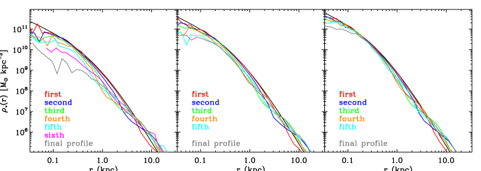
Figure 5.— Evolution of the satellite’s stellar density profile (top; logarithmic scale) and circular velocity profile (bottom; linear scale) for the same simulations shown in Fig. 4. Left: normal (SDSS) satellite. Center: $1\sigma$ dense satellite. Right: $2\sigma$ dense satellite. The profiles are computed at apocenter after each pericentric passage. Denser satellites are noticeably better preserved, both in their inner and outer structure. We do not plot the final circular velocity profile for the satellite because it is not meaningful when the satellite has merged with the host. Note the different radial scale on the upper and lower plots.

For a closer look at the changes in the internal structures of the satellites as they sink towards the center of the host galaxy, we show in Fig. 5 the satellite’s stellar density profiles $\rho_{\rm sat}(r)$ (upper) and circular velocity profiles $v_{\rm circ}(r)$ (lower) after each pericentric passage for the same runs as in Fig. 4. The profiles are computed at apocenter after the correspondingly labeled pericentric passage, e.g., the curves labeled “first” correspond to profiles at apocenter after the first pericentric pass. The circular velocity profiles clearly illustrate that the tidal effects during the first pericentric passage are confined to a satellite’s outer regions, while the later passages are responsible for the inner mass loss. The satellite with the standard density is stripped progressively more with each pericentric passage, resulting in a final central density that is reduced by about two orders of magnitude and a maximum circular velocity $v_{\mathrm{max}}$ that is reduced by 40% relative to the initial condition. The $1\sigma$ dense satellite is much less affected in density (although $v_{\mathrm{max}}$ is reduced by 30%), while the most compact ($2\sigma$ denser) satellite is stripped the least.

The effect of a black hole in the host on the satellite can also be seen clearly in the two upper-right panels of Fig. 5: while the stellar density profiles of the two satellites are well preserved at $\sim 0.5$ kpc, both profiles flatten on smaller scales due to interactions with the black hole. The typical radial scale on which we might expect the effects of the black hole to appear is given by an equation analogous to $M_{\star}(<r_{\mathrm{BH}})=2\,M_{\rm BH}$ in Sec. 2.1.3, with the stellar mass referring to that of the satellite. This gives $r_{\mathrm{BH}}=0.25\,a$ for the satellites we are considering, i.e. $\sim 0.15$ and 0.1 kpc for the $1\sigma$ and $2\sigma$ dense satellites, respectively, which indeed corresponds to the observed scale of the change in the density profile. We discuss the effects of black holes further in the next subsection.

3.3. Dependence on presence of central black holes

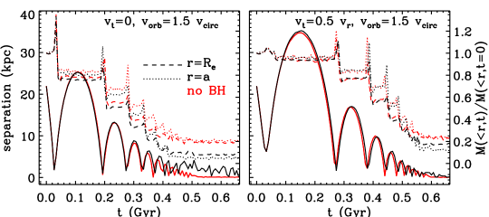
Figure 6.— Comparison of the orbital decay and stellar mass loss of a satellite as it is accreted onto a host galaxy with (black) and without (red) a central black hole. Two initial orbits are shown: radial (left panel) and $v_{t}/v_{r}=0.5$ (right panel). Black holes in host galaxies enhance the disruption efficiency for the satellite.

We have performed simulations without central black holes to quantify the effects of black holes in the host galaxies on the dynamics and disruption of infalling satellite galaxies. Fig. 6 compares results from runs with and without black holes for two orbits (left for radial orbit; right for $v_{t}/v_{r}=0.5$; both with orbital energy $v_{\mathrm{orb}}=1.5v_{\mathrm{circ}}$). The black hole has a non-negligible effect in the early evolution for the radial orbit because the satellite is brought to the host’s black hole immediately. Both the central (dotted curve) and outer (dashed curve) regions are somewhat more disrupted in the case where the host has a black hole. The differences between the two runs become more pronounced as the merger progresses: with successive pericentric passages the black hole exerts a stronger effect, widening the gap between the black and red curves on the left. By the time the merger is complete, the satellite stellar mass within its $R_{e}$ in the black hole run is only about half of that in the run without a black hole. The difference is even more pronounced at smaller radii; in fact, the black hole leads to a greater evacuation of mass within $a$ than within $R_{e}$, while the reverse is true for the run without a black hole.

The runs with $v_{t}/v_{r}=0.5$ (right panel) evolve differently. The satellite does not pass near the black hole on the first few pericentric passages, so the hole does not provide any shocking or stripping and there is no difference between the runs with and without a black hole. Once the orbit has decayed enough to bring the satellite close to the center of the host bulge, however, the black hole starts to exert its effect. The final result is again that the satellite is more destroyed when the host has a black hole, although the effect is not as strong as for the radial collision.

Figure 7.— Evolution of the ratio of the satellite’s stellar mass interior to the initial scale radius $a_{\mathrm{sat}}$ in runs with a black hole to the same quantity in runs without black holes. Two orbits are shown. Arrows mark first and second crossings of the black hole’s sphere of influence $r_{\mathrm{BH}}$ in the run with angular momentum. The ratio is seen to decrease noticeably between the crossings due to the tidal mass stripping by the black hole. The radial merger experiences crossings of $r_{\mathrm{BH}}$ at every pericentric passage, but the first 3 encounters are at high velocity and thus do not lead to significant tidal stripping.

To quantify the amount of satellite destruction due to the host’s black hole versus other tidal processes, we plot as a function of time in Fig. 7 the ratio of the satellite’s stellar mass within its initial scale radius $a$, $M_{\star,{\rm sat}}(<a,t)$, for the runs with a black hole relative to the same quantity in the runs without a black hole. For the radial merger (dashed line), this ratio decreases rapidly to about 25% after 0.4 Gyr due to the strong tidal effects exerted by the black hole on the accreting satellite. For the non-radial merger (solid line), this ratio stays at essentially unity until the satellite’s orbit has decayed enough to cross the hole’s sphere of influence ($r_{\mathrm{BH}}\sim 300$ pc) at $\approx 0.5$ Gyr. The first two crossings of $r_{\mathrm{BH}}$ (marked by arrows) correspond quite well to the initial decrease in $M_{\star,{\rm sat}}(<a;{\rm BH})$ relative to $M_{\star,{\rm sat}}(<a;\mathrm{no}\,{\rm BH})$. By the time the remnant has relaxed the run with a black hole has $\sim 50\%$ less mass within $a_{sat}$ relative to the run without a black hole. This is less of a dramatic reduction than in the radial merger because the black hole interacts fewer times with the center of the satellite in the run with angular momentum.

We have also considered the case where both the host and the satellite have central supermassive black holes. In this case, each black hole mass is set to $2\times 10^{-3}$ of its respective stellar bulge mass (see runs T5 & T6 in Table 1). The dense satellite (with satellite-to-host mass ratio of 1:10) is used for this run; if there is additional disruption of the satellite due to the presence of a black hole at its center, it will show up better in this case than in the lower-density one. We find that there is no substantive difference in the density profiles of either the host or satellite between the runs with one and two black holes. Our simulations, however, cannot follow the evolution of the system to the point at which three-body interactions among a supermassive black hole binary and stars start to scour out a core. The separation of the black holes at the hard binary stage is $r_{\rm hard}=G\mu/(4\sigma^{2})\approx 1$ pc for the parameters of our simulations; the highest force accuracy we use is $\epsilon=3$ pc (run T6 in Table 1), and even this scale can be significantly affected by two-body relaxation. Recent simulations by Merritt (2006) have studied the evolution of black hole binaries embedded in stellar spheroids with $\gamma$ profiles for a variety of black hole mass ratios and values of $\gamma$. The effect of a 1:10 binary ($q=0.1$) on a $\gamma=0.5$ profile is not very pronounced (his Fig. 5), implying that the surface brightness profiles presented here would not be strongly affected by core scouring.

3.4. Comparison to runs without dark matter

Figure 8.— Comparison of radial satellite accretion with (left) and without (right) dark matter halos. The run including dark matter (in both satellite and host) has $v_{\mathrm{orb}}=0.75\,v_{\mathrm{circ}}$ while the run without dark matter has $v_{\mathrm{orb}}=v_{\mathrm{circ}}$. Based purely on the results presented to this point, we expect the run with the higher ratio of $v_{\mathrm{orb}}/v_{\mathrm{circ}}$ to be more disrupted. The reverse is true, however, because the dark matter significantly deepens the host galaxy’s gravitational potential, leading to more pericentric passages for the satellite with dark matter and hence more severe mass losses.

Prior numerical studies on satellite accretion and their survival are focused on either purely dark matter subhalos (e.g., Hayashi et al. 2003; Kravtsov et al. 2004; Kazantzidis et al. 2004) or purely stellar systems (e.g., the pioneering work of White 1983; Balcells & Quinn 1990; Weinberg 1997; black holes are included in Holley-Bockelmann & Richstone 2000 and Merritt & Cruz 2001). In this subsection we compare the results of simulations ignoring the effects of dark matter to our full simulations (using stars, dark matter, and black holes) in order to quantify any potential differences. In general, simulations with only one primary component (stars or dark matter) are less expensive to perform than simulations with both components at a fixed force and mass resolution, so it is useful to assess whether including the effects of dark matter is necessary for understanding satellite evolution.

As outlined in Sec. 2.1, there is in fact good cause for thinking that including both dark matter and stellar components will lead to non-trivial differences from simulations with only dark matter halos or stellar bulges. The results of the previous sections indicate that one important parameter in determining whether or not a satellite is strongly disrupted is the number of pericentric passages it experiences before merging with the host bulge. Varying the depth of the host potential well is likely to change the number of orbits a satellite undergoes. Since orbital deceleration is governed by dynamical friction (equation 2), which is proportional to $M_{\rm sat}(t)/M_{\rm host}(t)$, and tidal stripping is likely to reduce $M_{\rm sat}$ by removing dark matter from outside the tidal radius, we expect the simulations with dark matter to have a slower orbital evolution and to go through more pericentric passages before merging than the equivalent runs without dark matter.

To quantify the effect of dark matter, we compare in Fig. 8 the results from a 3-component run (with dark matter, stars, and black hole) and a 2-component run without the dark matter halo (run L1 and T1 in Table 1). (The host and satellite either both have dark matter halos or both without.) The satellite for both runs is on a radial orbit with initial orbital velocity $v_{\mathrm{orb}}=0.75\,v_{\mathrm{circ}}$ (at $4R_{e}$). Note that the circular velocity $v_{\mathrm{circ}}$ is not equal in the two cases, as the dark matter contributes to the circular velocity. Fig. 8 shows that the satellite in the run with dark matter (left panel) experiences more pericentric passages before the final merger than the run without dark matter (right panel). Even though the satellites’ stellar masses interior to $R_{e}$ and $a$ are quite similar between the two runs after the first pericentric passage, the additional $\sim 3$ passages in the run with dark matter cause extra disruption. As a result, only 20-30% of the satellite’s stellar mass remains within its initial $R_{e}$ and $a$ after 0.2 Gyr in the 3-component run (dashed and dotted line in left panel) compared with the 70-80% in the run that ignored dark matter.

3.5. Other factors: mass ratio, inner density profile

We have tested a number of other parameters that can potentially affect the outcome of our satellite accretion simulations. Primary among these are the satellite-to-host mass ratio and the inner logarithmic slope $\gamma_{\star,\mathrm{s}}$ of the satellite’s density profile.

All the results presented thus far have assumed a satellite-to-host mass ratio of 1:10. We have performed a two-component test simulation (run T2 in Table 1) with a lower mass ratio of 1:33 and found qualitatively similar results. These lighter satellites lose their orbital energy on a longer time scale, however: it takes a factor of $\sim$1.5-2.5 longer for their stellar bulges to merge with and have observational impact on the host’s bulge. In a cosmological setting, we therefore expect the satellites with $\lesssim 5$% of the host mass to have less direct dynamical effect on the host than the more massive satellites despite their higher number density.

We have also performed several simulations (runs labeled “s” in Table 1) using a steeper $\rho\propto r^{-1.5}$ cusp for the initial stellar density of the satellite. As expected, these satellites suffer less tidal disruption than the $r^{-1}$ satellites studied thus far, but the net result is somewhat degenerate with decreasing $R_{e}$ of the satellite while fixing the $r^{-1}$ cusp. For example, our standard density satellite ($M_{\star}=3.3\times 10^{10}\,M_{\odot},\,a=0.76\,\mathrm{kpc},\,\gamma_{\star,\mathrm{s}}=1$) looks quite similar to a satellite with the same stellar mass but $\gamma_{\star,\mathrm{s}}=1.5$ and $a=1.35$ kpc: the densities differ by a maximum of 30% from 30 pc (our standard force softening) to 5 kpc. We include analyses of the runs with steeper satellite stellar density in the sections that follow below.

4. Observable consequences of satellite accretion

4.1. Surface brightness profiles

Figure 9.— Upper of each set of panels: Surface brightness profiles $\Sigma(R)$ of the host galaxy initially (thin solid curves) and after accretion of a satellite (computed from all stellar particles) for selected three-component runs. Lower of each set of panels: Same as top panels except it shows the corresponding fractional change between the initial and final $\Sigma(R)$ to accentuate the evolution of the surface brightness. Upper left: runs with varying orbital angular momentum at fixed orbital energy of $v_{\mathrm{orb}}/v_{\mathrm{circ}}=0.75$ and $\gamma_{\star,\mathrm{s}}=1.0$. The final central surface brightness is larger than the initial for all three runs but the amount of increase decreases with decreasing angular momentum. Upper right: runs with varying orbital angular momentum at fixed orbital energy of $v_{\mathrm{orb}}/v_{\mathrm{circ}}=1.50$ and $\gamma_{\star,\mathrm{s}}=1.0$. The increased orbital velocity leads to less deposition of satellite mass at the center of the remnant than in the $v_{\mathrm{orb}}/v_{\mathrm{circ}}=0.75$ case, and the radial collision results in a noticeably reduced inner central surface brightness. Lower left: runs with fixed orbital angular momentum ($v_{t}/v_{r}=0.5$) and fixed orbital energy ($v_{\mathrm{orb}}/v_{\mathrm{circ}}=1.5$) with $\gamma_{\star,\mathrm{s}}=1.0$ and varying satellite stellar density (i.e. varying $R_{e}$). The standard density satellite results in a reduced central surface brightness while the more compact satellites have dense centers that survive to the center of the host bulge, adding a large amount of mass. Lower right: runs with varying orbital angular momentum at fixed orbital energy of $v_{\mathrm{orb}}/v_{\mathrm{circ}}=1.5$ and $\gamma_{\star,\mathrm{s}}=1.5$. The final central surface brightness decreases for the radial run but increases for both runs with angular momentum.

As we have shown in Sec 3, the fate of a sinking satellite depends sensitively on a number of parameters including its orbital energy and angular momentum, its mass concentration, and the presence of black holes and dark matter halos. Even one dense satellite galaxy that finds its way to the center of a massive elliptical galaxy without being significantly disrupted can lead to a central density enhancement that is occasionally observed, so surface brightness profiles can serve as a useful diagnostic for structure formation models.

In Fig. 9 we illustrate how a single sinking satellite on a variety of orbits and with a range of stellar densities can modify the shallow surface brightness profile of a massive elliptical galaxy described in Sec 2. Fig. 10 is a busier summary plot for all of our 3-component simulations listed in Table 1 (including those in Fig. 9). Each curve is computed using the mean of twenty random projections of the merger remnant. In Fig. 9, the upper left panels compare a relatively bound satellite orbit at fixed energy ($v_{\mathrm{orb}}/v_{\mathrm{circ}}=0.75$) with varying angular momentum; the upper right panels show a more energetic orbit ($v_{\mathrm{orb}}/v_{\mathrm{circ}}=1.5$) with varying angular momentum; the lower left panels compare runs with identical orbital parameters ($v_{\mathrm{orb}}/v_{\mathrm{circ}}=1.5$, $v_{t}/v_{r}=0.5$) but varying initial satellite densities; and the lower right panels compare energetic ($v_{\mathrm{orb}}/v_{\mathrm{circ}}=1.5$) mergers with steeper satellite stellar density ($\gamma_{\star,\mathrm{s}}=1.5$) and varying angular momentum. The top panels show the absolute surface brightness profile $\Sigma(R)$ of the stellar component in the host galaxy initially (thin solid lines) and after satellite accretion (other lines; computed from all stellar particles in both the host and satellite); the bottom panels show the fractional changes between the initial and final $\Sigma(R)$.

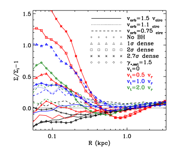
Figure 10.— Fractional change in the central surface brightness profile of a host galaxy after accretion of a satellite from all 3-component simulations listed in Table 1. The profiles show a wide spectrum of behavior on small radial scales, ranging from reduction in the central surface brightness for energetic and eccentric orbits, to sharp increases when the accreted satellite is relatively compact and dense initially. All the final surface brightness profiles have similar behavior at larger radii ($\gtrsim 2$ kpc), regardless of the central profile.

The general trend in the upper two sets of panels in Fig. 9 and in Fig. 10 is that satellites on more energetic or more eccentric (i.e. lower angular momentum) orbits are more destroyed due to the stronger tidal effects. This trend is consistent with the results in Sec. 3.1 and Figs. 2 and 3. While Figs. 2 and 3 illustrate the orbital decay and mass loss of the satellite, Figs. 9 and 10 show the net effect of the sinking satellite on the inner stellar distribution of the host galaxy.

A particularly noteworthy feature is seen in several cases in Fig. 9 and in Fig. 10: the central surface brightness of a core elliptical galaxy is actually reduced when a satellite is accreted on a relatively energetic ($v_{\mathrm{orb}}\gtrsim v_{\mathrm{circ}}$) and eccentric ($v_{t}\lesssim v_{r}$) orbit. Satellite accretion in this particular orbital parameter space is likely to occur infrequently, but it provides a potential mechanism for producing a minimum in the central surface brightness. Minima are seen in $\sim 5$% of the core galaxies (Lauer et al., 2002, 2005), although their physical scale tends to be at $\lesssim 100$ pc. A broader search in parameter space would be needed to determine whether the observed features can be more closely reproduced by specific combinations of parameters in this satellite accretion scenario.

The somewhat counter-intuitive reduction in central $\Sigma(R)$ via satellite accretion is the result of two processes. First, the accreting satellite clearly has to be largely destroyed so as to bring in little stellar mass to the host’s center. As Figs. 2 and 3 showed, energetic and eccentric orbits are effective means of destroying satellites. Second, as a satellite sinks via dynamical friction toward the host’s center, energy is transferred from the satellite to the host bulge, leading to gravitational heating that helps reduce the central stellar density in the host. Such satellite-host dynamical interaction and its effect on the bulge density and surface brightness profiles is therefore similar to that for dark matter halo density profiles, where dark matter subhalo accretion tends to heat the central cusp, reducing the central density, while deposition of the stripped mass and merging of the subhalo tends add to the central density (Ma & Boylan-Kolchin, 2004). In both cases (satellite accretion and dark matter subhalos) it is the competition between gravitational heating and mass deposition that determines whether the final profile is more dense or more diffuse than the initial profile.

The lower left panels of Fig. 9 show the strong effect of the initial satellite density on the host’s central $\Sigma(R)$. The satellite’s orbital decay, mass loss, and the evolution of its interior structure from the same three simulations were shown in Figs. 4 and 5. While the satellite on the SDSS $R_{e}-M_{\star}$ relation (thick solid lines) is disrupted and leads to a $\sim 10$% overall reduction in $\Sigma(R)$ in the inner $\sim 500$ pc (see paragraph above), the denser satellites (dashed and dotted lines) lead to a dramatic increase in the central surface brightness. Similar results are seen for satellites with $\gamma_{\star,\mathrm{s}}=1.5$ rather than $1.0$ with substantial angular momentum (lower right panels). Accretion of dense satellite – either with a steeper central stellar density profile or with a smaller $R_{e}$ – is therefore likely to add a dense remnant to the center of a core galaxy even when the tidal effects from the black holes are included. A small number of surface brightness profiles from the galaxy sample in Lauer et al. (2005) somewhat resemble the profiles of the $1-2\sigma$ dense satellites (e.g., NGC 3384). We suggest that satellite accretion offer a plausible explanation for the shapes of those profiles (see also Kormendy 1984).

4.2. Colors

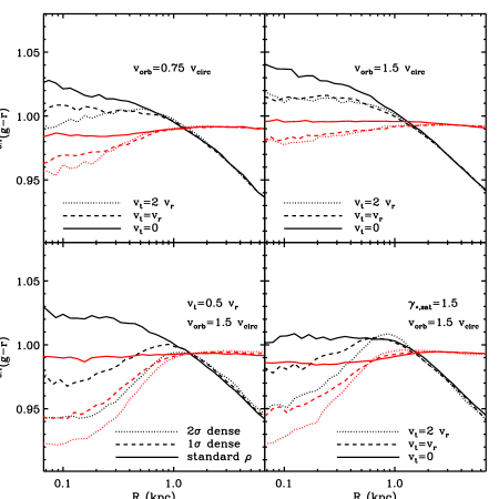
Figure 11.— ${}^{0.1}(g-r)$ color profiles for mergers with dark matter and a black hole, each averaged over 20 random projections. The host is assumed to have a color of 1.0 initially, while the satellite is given a color of 0.9 in each case. We consider two cases: no color gradient in either galaxy (red curves) or a color gradient of -0.1 mag/dex in both satellite and host (black curves). The panels are arranged as in Fig. 9. Upper left: $v_{\mathrm{orb}}=0.75\,v_{\mathrm{circ}}$ with varying $v_{t}/v_{r}$. Upper right: $v_{\mathrm{orb}}=1.5\,v_{\mathrm{circ}}$ with varying $v_{t}/v_{r}$. Lower left: $v_{\mathrm{orb}}=1.5\,v_{\mathrm{circ}},\,v_{t}/v_{r}=0.5$ with varying satellite density. Accretion of a compact satellite leads to a relatively bluer central remnant, while standard density satellites cause less change regardless of orbit. Lower right: $v_{\mathrm{orb}}=1.5\,v_{\mathrm{circ}}$ and $\gamma_{\star,\mathrm{s}}=1.5$ with varying $v_{t}/v_{r}$.

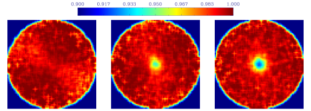
Figure 12.— Two-dimensional color map of the host bulge, viewed in the orbital plane, after accretion of a satellite with different initial densities: standard (left), $1\sigma$ denser (middle), and $2\sigma$ denser (right). The satellite orbit is identical for all three cases: $v_{t}/v_{r}=0.5,\,v_{\mathrm{orb}}/v_{\mathrm{circ}}=1.5$; neither galaxy is given an initial color gradient. Each panel is (6.66 kpc)²; each pixel corresponds to 0.1 kpc. The cores of the 1 and 2$\sigma$ dense satellites survive to leave a visible core bluer by $\approx 0.05-0.08$ mag. Close inspection of the left panel shows that although the satellite with standard density does not survive to the center, it leaves faint plumes of stripped stars (light red) at very low color contrast ($\approx 0.01$ mag bluer).

Both the average color and the color gradients in elliptical galaxies contain vital information about their star formation and assembly histories. For instance, the slope and scatter along the red sequence in the color-magnitude relation (CMR) is a useful diagnostic of how pre-existing early-type galaxies build up larger elliptical galaxies, as this merging would tend to average the colors and thus wash out any correlations (Bower et al., 1998). Monolithic collapse models generally predict steep color gradients originating from strong radial metallicity gradients (Larson, 1974; Carlberg, 1984). The case is not as clear-cut in hierarchical models, as the effects of metallicity gradients established by gas-rich mergers can be diluted by violent relaxation and mixing in gas-poor mergers. In general, the distribution of a satellite’s stars should affect the local color of a host in a way that depends on the satellite orbit and density. If the satellite sinks to the host’s center without substantial mass loss, for example, the resulting color on small scales will be close to the satellite’s initial color. If, on the other hand, the satellite is disrupted outside the host’s core, the remnant’s central color will be essentially identical to that of the host initially.

We investigate the changes in galaxy colors due to satellite accretion by assigning initial colors to the host and satellite and then computing the remnant’s color under the assumption of no change in color due to stellar population evolution. This method isolates the effects of mixing in the mergers. We assign the initial galaxies ${}^{0.1}(g-r)$ colors of 0.9 for the satellite and 1.0 for the host. The observed CMR slope from SDSS in ${}^{0.1}(g-r)$ is -0.022 mag/dex (Hogg et al., 2004), meaning we have slightly accentuated the expected color difference between the host and satellite given their masses. When we consider galaxies with initial color gradients, this color corresponds to the color measured within the effective radius.

Fig. 11 shows the circularly-averaged color profiles for the same sets of simulations shown in Fig. 9; as in Fig. 9, each curve is computed using the mean of twenty random projections of the remnant. The red curves assume no initial color gradient for either galaxy and show that the properties of the satellite and its orbit make a significant difference in the color of the inner $\sim 1$ kpc of the remnant. The dense satellites (lower left panel) and $\gamma_{\star,\mathrm{s}}=1.5$ satellites (lower right panel) lead to a bluer center, a result of their undisrupted cores settling to the center of the host. The runs with standard density and varying orbital properties show less pronounced central differences. For all simulations, the ${}^{0.1}(g-r)$ color at large radii is about 0.99, so $\Delta$ color $\approx 0.01$ mag.

The black curves in Fig. 11 assume each galaxy initially had a color gradient of $-0.1$ mag/dex and show how these gradients evolve as a result of the merger. In the runs with lower $v_{\mathrm{orb}}$ (upper left panel), the gradient is diluted somewhat in the center but only the run with the highest angular momentum causes a central inversion. None of the runs at higher $v_{\mathrm{orb}}$ and $\gamma_{\star,\mathrm{s}}=1.0$ (upper right panel) have a central color inversion, but the color profile does flatten toward the center. The runs with higher stellar density or steeper inner stellar density slope show a marked change in central color at approximately $R_{e}/5$ (as in the case without initial gradients). The general trend we see is to weaken the central color gradients while affecting the outer regions less strongly. This weakening is in agreement with the trend reported in White (1980). Luminous elliptical galaxies do tend to have slightly weaker gradients in metallicity (Carollo et al., 1993) and color (Lauer et al., 2005) than faint ellipticals galaxies, perhaps as a result of this mixing process.

To quantify the color signatures of satellite accretion further, we have also examined two-dimensional color maps of the hosts to look for features that are not evident in the 1-dimensional color profiles shown in Fig. 11. A set of such maps (viewed in the orbital plane) is shown in Fig. 12, comparing the three runs with different initial satellite densities. The initial colors are the same as for Fig. 11. The 2$\sigma$ dense satellite (right panel) sinks to the center without significant disruption, leaving an observable core of $\approx 0.5$ kpc in the remnant. Even the $1\sigma$ dense satellite (center panel) leaves an observable color signature in the core, although it is both smaller and and less concentrated than the $2\sigma$ dense core. By contrast, the standard density satellite is largely destroyed and leaves no core in the remnant (left panel of Fig. 12), as was previously seen in other ways (e.g., Figs 4 and 9). Close inspection, however, shows faint plumes of bluer features at low color differences ($\approx 0.01-0.02$ mag) from stripped stars of the torn-up satellite. The axis of the plume correlates well with the orbit of the satellite over its final several pericentric passages (which are quite radial).

4.3. Additional observable properties: intra-cluster light and kinematic structure

Many massive galaxies at or near the centers of clusters are cD galaxies with extended stellar envelopes, often extending out to hundreds of kpc. Satellite accretion onto cluster halos (and subsequent satellite disruption) contributes, perhaps significantly, to this intracluster light (ICL; e.g., Merritt 1984; Moore et al. 1996; Gregg & West 1998; Gnedin 2003; Zibetti et al. 2005; Mihos et al. 2005). Our initial setup for the galaxies is biased against producing ICL in the sense that we truncate the stellar bulge, removing the stars that are at large radii (and thus are least bound). This truncation eliminates the stars that would be most easily removed from the satellite and deposited at large radii relative to the center of the remnant. Nevertheless, it is not inconceivable that a fraction of stars in our mergers is deposited out to large radii, contributing to an ICL component.

The remnants in all of our simulations show excess stellar mass at large radii ($>3R_{e}$ for the initial host profile), as is visible in the lower panels of Fig. 9 and Fig. 10. Although the excess is relatively small – of order 15-25% – it shows that the star particles do get deposited significantly outside of the host’s effective radius, indicating that tidal stripping of merging satellites can contribute to ICL. For cases with $v_{\mathrm{orb}}=1.5\,v_{\mathrm{circ}}$, the stellar mass that belonged to the satellite tends to be distributed with a larger characteristic radius than the mass that belonged to the host. Simulations of repeated satellite accretion in a cluster environment would likely yield a significant ICL component originating from the tidal stripping of satellites. Analyses of cosmological simulations have shown this process to yield some ICL (Sommer-Larsen et al., 2005; Willman et al., 2004; Rudick et al., 2006); future higher-resolution simulations should shed more light on the origin of the ICL.

Many elliptical galaxies are observed to have kinematically distinct substructure at their centers (kinematically decoupled cores, KDCs); often these cores counter-rotate relative to the galaxy (de Zeeuw & Franx, 1991). A recent survey by the SAURON team of 48 nearby ($cz<3000\,{\rm km}\,{\rm s}^{-1}$) E/S0 galaxies revealed a wide range of kinematic substructure, from $\sim 100$ pc young cores in fast rotators to kpc-scale, old KDCs in slow rotators (McDermid et al., 2006). We have tested for such substructure by making velocity maps of our remnants. None of them exhibit a KDC; the velocity fields in all cases are consistent with zero net rotation and no kinematic subcomponents. Intriguingly, the three most luminous galaxies in the SAURON sample, including M87, do not have KDCs. Since this type of galaxy is similar to our initial host, our simulations are in this sense in good agreement with the SAURON observations.

A broader question to be explored in future work is the origin and fragility of KDCs in slow-rotating galaxies. Gas physics could play a role in creating KDCs: Hernquist & Barnes (1991), Jesseit et al. (2006), and Cox et al. (2006) have demonstrated that simulations of binary disk galaxy mergers with gas can lead to kinematic substructure in the remnants. In dissipationless simulations, Balcells & Quinn (1990) have shown that a dense satellite sinking to the center of a more diffuse host can create a counter-rotating core if a large initial rotation of $V/\sigma_{0}=0.75$ for the satellite and 0.4 for the host are used and the merging orbits are retrograde. It is somewhat difficult to discern from the SAURON results what fraction of slow-rotators should have KDCs given the sample size (12 slow-rotators). If their results are representative, however, then it is possible that any KDC would be erased if massive ellipticals are built by multiple generations of merging.

One satellite accretion event with mass ratio 1:10 does not strongly affect the radius or velocity dispersions of the remnant nor does it increase $M_{\star}$ substantially, meaning scaling relations such as the fundamental plane or its projections do not change notably. Remnants of major mergers (mass ratio 1:1-1:3), on the other hand, can have very different properties depending on energy or angular momentum of the merger orbit (Boylan-Kolchin et al., 2006). Checking the evolution of sizes, stellar masses, and velocity dispersion over a sequence of merger events would therefore be a good test of the evolution of scaling laws such as the Faber-Jackson and $M_{\mathrm{BH}}-\sigma_{e}$ relations.

5. Conclusions and Discussion

In this paper we have used dissipationless simulations to examine in detail and over a wide range of parameter space the case-by-case outcome of a single satellite elliptical galaxy accreting onto a core elliptical galaxy. We have taken special care to explore cosmologically relevant orbital parameters and to set up realistic galaxy models that include all three relevant dynamical components: dark matter halos, stellar bulges, and central massive black holes. The main results in this paper are as follows:

(i) Satellites on more energetic or more eccentric (lower angular momentum) orbits are destroyed more efficiently due to the stronger tidal effects from the host spheroid and the central black hole (see Figs. 2, 3, 9-12).

(ii) Denser satellite galaxies – those with either a smaller $R_{e}$ or a steeper inner slope – survive significantly better (see Figs. 4, 5, 9-12). For instance, the standard density satellite in Fig. 4 loses more mass by its 3rd pericentric passage than the total mass loss in the $2\sigma$ dense satellite during its entire orbital evolution.

(iii) A supermassive black hole at the center of the host galaxy significantly increases the efficiency with which an accreting satellite is destroyed (see Figs. 6, 7, 10). Without a central black hole, luminous elliptical galaxies would have more difficulty in protecting their shallow inner profile (however formed initially) from steepening due to mass deposit through satellite accretion, in agreement with previous 2-component numerical work (Holley-Bockelmann & Richstone, 2000; Merritt & Cruz, 2001).

(iv) Ignoring dark matter halos in the galaxy models causes significant differences primarily because dark matter halos lead to higher orbital velocities for a fixed ratio of $v_{\mathrm{orb}}/v_{\mathrm{circ}}$ (see Fig. 8). Satellites with increased orbital velocity complete more orbits before merging with the host, resulting in greater destruction of the satellite galaxy.

(v) Our overall conclusion is that the accretion of a single satellite elliptical galaxy (1/30 to 1/10 mass of the host) can result in a broad range of changes, in both signs, in the surface brightness profile $\Sigma(R)$ and color of the central part of an elliptical galaxy, as summarized in Figs. 10-12.

More specifically, Figs. 10-12 show that when a black hole is included in the host galaxy and when the satellite and host are both on the SDSS stellar size-mass relation, the fractional change in $\Sigma(R)$ in the inner $\sim 500$ pc of the host galaxy upon satellite accretion ranges from $\sim-20\%$ to $\sim+40\%$ When more compact satellites are considered in accordance to the large scatter about the SDSS size-mass relation, the inner $\Sigma(R)$ of the host galaxy can increase by more than 100%. Since accretion of a single satellite adds little mass and luminosity to the host, we suggest that a “core” galaxy at $M_{v}\sim-22$ can potentially transition into a galaxy with power-law characteristics at a comparable luminosity by accretion of a relatively compact and massive ($\sim$ 1:10) satellite. A core-in-core structure would provide particularly strong evidence for this process (see also Kormendy 1984).

The strong dependence of satellite mass loss on the satellite’s density relative to the host and the inclusion of black holes has broader implications, for example, in interpreting the connection between dark matter subhalos and galaxies in cosmological simulations that model only dark matter. Dark matter subhalos in these simulations are often stripped to the point of not being distinguishable from the host dark matter halo. In semi-analytic models of galaxy formation (e.g. Gao et al. 2004; Wang et al. 2006), these subhalos are tracked as “galaxies” by either following the most bound particle of the subhalo or extrapolating their positions and velocities using information from previous timesteps. The results from our three-component (dark matter+stars+black hole) non-cosmological simulations suggest that the properties of the observable stellar component in the simulations are very sensitive to their assumed initial properties, and in particular, to the initial stellar density assigned to the galaxies and the inclusion of black holes in the host galaxies. Future work that incorporates the results presented here into a full cosmological context should be valuable.

Appendix A Properties of two-component $\gamma$ models

Figure 13.— Left: Density profiles of $\gamma$-profiles used in this paper. Solid curves show the untruncated profiles ($\gamma_{\star,\mathrm{h}}=0.5,\,M=3.33\times 10^{11}\,M_{\odot},\,a=2.33\,\mathrm{kpc}$ for the bulge, $\gamma_{\mathrm{DM}}=1,\,M=3.33\times 10^{12}\,M_{\odot},\,a=33.3\,\mathrm{kpc}$ for the halo). The dotted lines show truncated profiles for the halo (from left to right, $a_{DM}^{\prime}=66.7,\,133,\,333$ kpc; 133 kpc is used for the host halos in the simulations), while the dot-dot-dot-dash lines show truncated profiles for the bulge (from left to right, $a_{\star}^{\prime}=33.3,\,83.3,\,167$ kpc; 167 kpc is used for the host bulges in the simulations). Note that as $a^{\prime}\rightarrow a$ (leftmost dotted curve), the inner density amplitude drops but the slope remains the same. Right: Stability test of a standard satellite for our simulations. Plotted are the initial density profiles (solid curves) for the stellar bulge and dark matter halo, as well as the evolved profiles at t = 1 Gyr (dashed curves). The force softening for this run is $\epsilon$ = 33 pc. The model is stable on all scales larger than $\sim 2.5\,\epsilon$.

A.1. Untruncated Models

Dehnen (1993, Appendix B) gives several useful formulae for numerically computing quantities such as surface brightness profiles and projected velocity dispersions for standard $\gamma$ models. His integral transforms can be readily extended to both full and truncated two-component $\gamma$ models, as we show here. We first consider the untruncated models composed of three components (dark matter, stars, and a central black hole), with $\rho_{\mathrm{DM}}=\rho(\gamma_{\mathrm{DM}},M_{\mathrm{DM}},a_{\mathrm{DM}};r)$ and $\rho_{\star}=\rho(\gamma_{\star},M_{\star},a_{\star};r)$; we set Newton’s constant $G$ to unity in the calculations that follow.

Since the spatial structure of each component is unaffected by the other component, the formulae in Dehnen (1993) for surface density and cumulative surface density are valid for each component of the untruncated two-component models. Computing the projected velocity dispersion is somewhat more complicated, as the velocity structure of a system is determined by the total gravitational potential.

The projected stellar velocity dispersion $\sigma_{p,\star}(R)$ as a function of projected radius $R$ can be computed from the Jeans equation:

$$\sigma_{p,\star}^{2}(R) = \frac{2}{\Sigma_{\star}(R)}\int_{R}^{\infty}\rho_{\star}\sigma_{r}^{2}(r)\frac{r}{(r^{2}-R^{2})^{1/2}}\,dr$$ (A1)

$$= \frac{2}{\Sigma_{\star}(R)}\int_{R}^{\infty}\frac{\rho_{\star}M_{\mathrm{tot}}(r)}{r^{2}}(r^{2}-R^{2})^{1/2}\,dr$$ (A2)

(c.f. Tremaine et al., 1994, eqns. 27-29), where $\sigma_{r}^{2}(r)$ is the stellar radial velocity dispersion. The total mass profile can be split into three parts, $M_{\mathrm{tot}}(r)=M_{\star}(r)+M_{\mathrm{DM}}(r)+M_{\mathrm{BH}}(r)$, meaning the integral can be split into three pieces: $\sigma_{p,\star}^{2}(r)=s_{p,\star}^{2}(r)+s_{p,\mathrm{DM}}^{2}(r)+s_{p,BH}^{2}(r)$. The first term is the projected dispersion for the one-component case (e.g., Dehnen’s eqn. 18), though a singularity in the integrand means it can be much more easily computed using his eqn. B2. The third term can be mapped into an integral similar to that of the first term (Tremaine et al., 1994, eqns. 49-51) and then computed using Dehnen’s eqn. B2. This leaves only one piece to be computed:

$$s_{p,\mathrm{DM}}^{2}(r)=\frac{2}{\Sigma_{\star}(R)}\int_{R}^{\infty}\frac{\rho_{\star}M_{\mathrm{DM}}(r)}{r^{2}}(r^{2}-R^{2})^{1/2}\,dr\,.$$ (A3)

This term is difficult to compute numerically because of the limits of integration. Following Dehnen, we make the substitution

$$t^{2}\equiv\frac{r}{r+a_{\star}}(s+1)-s\,,$$ (A4)

with $s\equiv R/a_{\star}$, and take $a_{\star}=1=M_{\star}$. Eqn. A3 then becomes

$$s_{p,\mathrm{DM}}^{2}(R) = \frac{3-\gamma_{\star}}{\pi\Sigma_{\star}(R)}\frac{M_{\mathrm{DM}}M_{\star}}{a_{\star}^{3}}(1+s)^{-(5/2-\gamma_{\star})}$$ (A5)

$$\times \int_{0}^{1}(1-t^{2})^{3}(t^{2}+s)^{1-\gamma_{\star}-\gamma_{DM}}\,[t^{2}(1-a_{DM})+s+a_{DM}]^{\gamma_{DM}-3}\,t^{2}\,\sqrt{2s+t^{2}(1-s)}\,dt\,,$$

and numerical integration is straightforward.

A.2. Truncated Models

As described in the main text, we truncate the density profiles of our models by subtracting off a second $\gamma$ profile: assuming the desired density profile is $\rho_{i}(\gamma,M,a;r)$, we take the truncated density profile to be

$$\rho_{i}(r)=\rho_{i}(\gamma,M,a;r)-\rho_{i}(\gamma^{\prime},M^{\prime},a^{\prime};r)\,.$$ (A6)

In order to preserve the same inner density structure, we require that $\gamma^{\prime}=\gamma$, $M^{\prime}\leq M$, and $a^{\prime}\gg a$. By varying $M^{\prime}$ and $a^{\prime}$, we can control the truncation. The maximum radius for one component in these models is given by

$$r_{\mathrm{max}}=a\frac{\Delta-1}{1-\frac{a}{a^{\prime}}\Delta}$$ (A7)

where

$$\Delta\equiv\left[\frac{M}{M^{\prime}}\left(\frac{a^{\prime}}{a}\right)^{3-\gamma}\right]^{1/(4-\gamma)}\,.$$ (A8)

The left panel of Fig. 13 shows the profiles, both untruncated and truncated, for the dark matter halos and bulges used in several of the simulations presented in this paper. The numerical stability of one of the satellite models is demonstrated in the right panel of Fig. 13: there is no evolution in the density profile for scales $\gtrsim 2.5\,\epsilon$. The host models are equally stable, both with and without black holes.

Since the truncated models do not have infinite extent, many of the integration limits change. For example, the velocity dispersion has $\int_{r}^{\infty}\rightarrow\int_{r}^{r_{\mathrm{max}}}$, where $r_{\mathrm{max}}$ is given by eqn. A7. Projected quantities therefore have an upper limit of $r_{\mathrm{max}}$ rather than $\infty$, or equivalently, $t_{\mathrm{max}}=t(r_{\mathrm{max}})$ rather than $t_{\mathrm{max}}=1$. The calculations are also changed by the addition of the second profile, which essentially serves as two additional mass components. For example, now $M_{\mathrm{tot}}\rightarrow M_{\star}-M_{\star^{\prime}}+M_{\mathrm{DM}}-M_{\mathrm{DM}^{\prime}}+M_{\mathrm{BH}}$ and $\rho_{\star}(r)\rightarrow[\rho_{\star}(r)-\rho_{\star^{\prime}}(r)]$ (and similarly for $\rho_{\mathrm{DM}}$). Velocity dispersions can be computed substituting these relations into the appropriate equations given above.

The surface brightness for a truncated model is similarly given by

$$\Sigma_{\star}(R)=2\int_{R}^{r_{\mathrm{max}}}\frac{\rho(r)}{(r^{2}-R^{2})^{1/2}}\,r\,dr\,$$ (A9)

so introducing a truncation for the bulge in the form of $\rho_{\star^{\prime}}(r)=\rho(\gamma_{\star^{\prime}},M_{\star^{\prime}},a_{\star^{\prime}};r)$ is simply a linear operation and

$$\Sigma_{\star}(R)=\Sigma_{\star}(R)-\Sigma_{\star^{\prime}}(R)\,.$$ (A10)

References

- Balcells & Quinn (1990) Balcells, M., & Quinn, P. J. 1990, ApJ, 361, 381
- Begelman et al. (1980) Begelman, M. C., Blandford, R. D., & Rees, M. J. 1980, Nature, 287, 307
- Bender et al. (1992) Bender, R., Burstein, D., & Faber, S. M. 1992, ApJ, 399, 462
- Benson (2005) Benson, A. J. 2005, MNRAS, 358, 551
- Binney & Tremaine (1987) Binney, J., & Tremaine, S. 1987, Galactic Dynamics (Princeton, NJ, Princeton University Press)
- Bower et al. (1998) Bower, R. G., Kodama, T., & Terlevich, A. 1998, MNRAS, 299, 1193
- Boylan-Kolchin et al. (2005) Boylan-Kolchin, M., Ma, C.-P., & Quataert, E. 2005, MNRAS, 362, 184
- Boylan-Kolchin et al. (2006) —. 2006, MNRAS, 369, 1081
- Carlberg (1984) Carlberg, R. G. 1984, ApJ, 286, 403
- Carollo et al. (1993) Carollo, C. M., Danziger, I. J., & Buson, L. 1993, MNRAS, 265, 553
- Chatterjee et al. (2002) Chatterjee, P., Hernquist, L., & Loeb, A. 2002, Phys. Rev. Lett., 88, 121103
- Cox et al. (2006) Cox, T. J., Dutta, S. N., Di Matteo, T., Hernquist, L., Hopkins, P. F., Robertson, B., & Springel, V. 2006, astro-ph/0607446
- Davies et al. (1983) Davies, R. L., Efstathiou, G., Fall, S. M., Illingworth, G., & Schechter, P. L. 1983, ApJ, 266, 41
- de Vaucouleurs (1948) de Vaucouleurs, G. 1948, Annales d’Astrophysique, 11, 247
- de Zeeuw & Franx (1991) de Zeeuw, T., & Franx, M. 1991, ARA&A, 29, 239
- Dehnen (1993) Dehnen, W. 1993, MNRAS, 265, 250
- Dekel et al. (2003) Dekel, A., Devor, J., & Hetzroni, G. 2003, MNRAS, 341, 326
- Djorgovski & Davis (1987) Djorgovski, S., & Davis, M. 1987, ApJ, 313, 59
- Dressler et al. (1987) Dressler, A., Lynden-Bell, D., Burstein, D., Davies, R. L., Faber, S. M., Terlevich, R., & Wegner, G. 1987, ApJ, 313, 42
- Ebisuzaki et al. (1991) Ebisuzaki, T., Makino, J., & Okumura, S. K. 1991, Nature, 354, 212
- Faber & Jackson (1976) Faber, S. M., & Jackson, R. E. 1976, ApJ, 204, 668
- Faber et al. (1997) Faber, S. M. et al. 1997, AJ, 114, 1771
- Ferrarese et al. (2006) Ferrarese, L. et al. 2006, ApJS, 164, 334
- Ferrarese & Merritt (2000) Ferrarese, L., & Merritt, D. 2000, ApJ, 539, L9
- Gao et al. (2004) Gao, L., De Lucia, G., White, S. D. M., & Jenkins, A. 2004, MNRAS, 352, L1
- Gebhardt et al. (2000) Gebhardt, K. et al. 2000, ApJ, 539, L13
- Gebhardt et al. (2003) —. 2003, ApJ, 583, 92
- Genzel et al. (2001) Genzel, R., Tacconi, L. J., Rigopoulou, D., Lutz, D., & Tecza, M. 2001, ApJ, 563, 527
- Gnedin (2003) Gnedin, O. Y. 2003, ApJ, 589, 752
- Gnedin et al. (1999) Gnedin, O. Y., Hernquist, L., & Ostriker, J. P. 1999, ApJ, 514, 109
- Gnedin & Ostriker (1999) Gnedin, O. Y., & Ostriker, J. P. 1999, ApJ, 513, 626
- Gregg & West (1998) Gregg, M. D., & West, M. J. 1998, Nature, 396, 549
- Häring & Rix (2004) Häring, N., & Rix, H. 2004, ApJ, 604, L89
- Hausman & Ostriker (1978) Hausman, M. A., & Ostriker, J. P. 1978, ApJ, 224, 320
- Hayashi et al. (2003) Hayashi, E., Navarro, J. F., Taylor, J. E., Stadel, J., & Quinn, T. 2003, ApJ, 584, 541
- Hernquist (1990) Hernquist, L. 1990, ApJ, 356, 359
- Hernquist & Barnes (1991) Hernquist, L., & Barnes, J. E. 1991, Nature, 354, 210
- Hogg et al. (2004) Hogg, D. W. et al. 2004, ApJ, 601, L29
- Holley-Bockelmann & Richstone (2000) Holley-Bockelmann, K., & Richstone, D. O. 2000, ApJ, 531, 232
- Jesseit et al. (2006) Jesseit, R., Naab, T., Peletier, R., & Burkert, A. 2006, astro-ph/0606144
- Kauffmann et al. (2003) Kauffmann, G. et al. 2003, MNRAS, 341, 33
- Kazantzidis et al. (2004) Kazantzidis, S., Mayer, L., Mastropietro, C., Diemand, J., Stadel, J., & Moore, B. 2004, ApJ, 608, 663
- Khochfar & Burkert (2006) Khochfar, S., & Burkert, A. 2006, A&A, 445, 403
- Kormendy (1984) Kormendy, J. 1984, ApJ, 287, 577
- Kormendy & Bender (1996) Kormendy, J., & Bender, R. 1996, ApJ, 464, L119
- Kravtsov et al. (2004) Kravtsov, A. V., Gnedin, O. Y., & Klypin, A. A. 2004, ApJ, 609, 482
- Larson (1974) Larson, R. B. 1974, MNRAS, 166, 585
- Lauer (1988) Lauer, T. R. 1988, ApJ, 325, 49
- Lauer et al. (1995) Lauer, T. R. et al. 1995, AJ, 110, 2622
- Lauer et al. (2005) —. 2005, AJ, 129, 2138
- Lauer et al. (2006) —. 2006, astro-ph/0606739
- Lauer et al. (2002) —. 2002, AJ, 124, 1975
- Ma & Boylan-Kolchin (2004) Ma, C., & Boylan-Kolchin, M. 2004, Phys. Rev. Lett., 93, 021301
- Magorrian et al. (1998) Magorrian, J. et al. 1998, AJ, 115, 2285
- McDermid et al. (2006) McDermid, R. M. et al. 2006, New Astronomy Review, 49, 521
- Merritt (1984) Merritt, D. 1984, ApJ, 276, 26
- Merritt (1985) —. 1985, ApJ, 289, 18
- Merritt (2006) —. 2006, astro-ph/0603439
- Merritt & Cruz (2001) Merritt, D., & Cruz, F. 2001, ApJ, 551, L41
- Mihos et al. (2005) Mihos, J. C., Harding, P., Feldmeier, J., & Morrison, H. 2005, ApJ, 631, L41
- Milosavljević & Merritt (2001) Milosavljević, M., & Merritt, D. 2001, ApJ, 563, 34
- Moore et al. (1996) Moore, B., Katz, N., Lake, G., Dressler, A., & Oemler, Jr., A. 1996, Nature, 379, 613
- Navarro et al. (1997) Navarro, J. F., Frenk, C. S., & White, S. D. M. 1997, ApJ, 490, 493
- Ostriker et al. (1972) Ostriker, J. P., Spitzer, L. J., & Chevalier, R. A. 1972, ApJ, 176, L51
- Ostriker & Tremaine (1975) Ostriker, J. P., & Tremaine, S. D. 1975, ApJ, 202, L113
- Padmanabhan et al. (2004) Padmanabhan, N. et al. 2004, New Astronomy, 9, 329
- Quinlan & Hernquist (1997) Quinlan, G. D., & Hernquist, L. 1997, New Astronomy, 2, 533
- Ravindranath et al. (2001) Ravindranath, S., Ho, L. C., Peng, C. Y., Filippenko, A. V., & Sargent, W. L. W. 2001, AJ, 122, 653
- Rudick et al. (2006) Rudick, C. S., Mihos, J. C., & McBride, C. 2006, astro-ph/0605603
- Shen et al. (2003) Shen, S., Mo, H. J., White, S. D. M., Blanton, M. R., Kauffmann, G., Voges, W., Brinkmann, J., & Csabai, I. 2003, MNRAS, 343, 978
- Sommer-Larsen et al. (2005) Sommer-Larsen, J., Romeo, A. D., & Portinari, L. 2005, MNRAS, 357, 478
- Springel (2005) Springel, V. 2005, MNRAS, 364, 1105
- Springel et al. (2005) Springel, V., Di Matteo, T., & Hernquist, L. 2005, MNRAS, 361, 776
- Taffoni et al. (2003) Taffoni, G., Mayer, L., Colpi, M., & Governato, F. 2003, MNRAS, 341, 434
- Taylor & Babul (2001) Taylor, J. E., & Babul, A. 2001, ApJ, 559, 716
- Tremaine et al. (1994) Tremaine, S., Richstone, D. O., Byun, Y., Dressler, A., Faber, S. M., Grillmair, C., Kormendy, J., & Lauer, T. R. 1994, AJ, 107, 634
- Velazquez & White (1999) Velazquez, H., & White, S. D. M. 1999, MNRAS, 304, 254
- Wang et al. (2006) Wang, L., Li, C., Kauffmann, G., & De Lucia, G. 2006, astro-ph/0603546, 785
- Weinberg (1994) Weinberg, M. D. 1994, AJ, 108, 1403
- Weinberg (1997) —. 1997, ApJ, 478, 435
- White (1980) White, S. D. M. 1980, MNRAS, 191, 1
- White (1983) —. 1983, ApJ, 274, 53
- Willman et al. (2004) Willman, B., Governato, F., Wadsley, J., & Quinn, T. 2004, MNRAS, 355, 159
- York et al. (2000) York, D. G. et al. 2000, AJ, 120, 1579
- Zibetti et al. (2005) Zibetti, S., White, S. D. M., Schneider, D. P., & Brinkmann, J. 2005, MNRAS, 358, 949