Intrinsic Short time scale variability in W3(OH) Hydroxyl masers

Abstract

We have studied the OH masers in the star forming region, W3(OH), with data obtained from the Very Long Baseline Array (VLBA). The data provide an angular resolution of $\sim$5 mas, and a velocity resolution of 106 m s^-1. A novel analysis procedure allows us to differentiate between broadband temporal intensity fluctuations introduced by instrumental gain variations plus interstellar diffractive scintillation, and intrinsic narrowband variations. Based on this 12.5 hours observation, we are sensitive to variations with time scales of minutes to hours. We find statistically significant intrinsic variations with time scales of $\sim$15–20 minutes or slower, based on the velocity-resolved fluctuation spectra. These variations are seen predominantly towards the line shoulders. The peak of the line profile shows little variation, suggesting that they perhaps exhibit saturated emission. The associated modulation index of the observed fluctuation varies from statistically insignificant values at the line center to about unity away from the line center. Based on light-travel-time considerations, the 20-minute time scale of intrinsic fluctuations translates to a spatial dimension of $\sim$2–3 AU along the sight-lines. On the other hand, the transverse dimension of the sources, estimated from their observed angular sizes of about $\sim$3 mas, is about 6 AU. We argue that these source sizes are intrinsic, and are not affected by interstellar scatter broadening. The implied peak brightness temperature of the 1612/1720 maser sources is about $\sim 2\times 10^{13}$ K, and a factor of about five higher for the 1665 line.

1. Introduction

Interstellar hydroxyl maser sources are found in the Galaxy and many external galaxies. In the Galaxy, these sources are associated with star forming regions (predominantly in the 1665 and 1667 MHz lines), IR and late type stars (mainly at 1612 MHz) and supernova remnants (exclusively at 1720 MHz).

Numerous VLBI observations (e.g., Gwinn et al 1988; Fish et al 2005; 2006) have indicated that the apparent angular sizes of OH masers increase with distance in the Galaxy. OH maser sources in the inner Galaxy show larger angular sizes compared to sources in the outer Galaxy. These facts strongly suggest that the observed angular size is strongly dependent on interstellar scatter broadening. Some years ago, Burke et al (1968) and Gwinn et al (1988) have proposed that the apparent broadening of masers shows a wavelength dependence $\propto\lambda^{2}$, based on OH maser sizes at 1665 MHz and $H_{2}O$ maser sizes at 23 GHz. These data suggest that interstellar scattering is the dominant cause for the observed angular sizes of these sources.

Desai, Gwinn & Diamond (1994) used the VLBA to study the details of the interstellar broadening of the OH masers in the distant ($\sim$14 kpc) HII region W49N. Anisotropic broadening was observed with the orientation of the minor axis preferentially parallel to the Galactic plane, an additional confirmation of the influence of interstellar scattering on the scattered sizes. An unambiguous determination of the intrinsic sizes of OH maser sources would represent an important input in understanding the OH maser pump and emission mechanism.

In addition to the intrinsic sizes, an important property of the masers that provides information about the pumping mechanism is the variability of the maser intensity as a function of time. Variability on long time scales (weeks to months) has been discussed by numerous investigators (Schwartz, Harvey & Barrett 1974; Coles, Rumsey & Welch 1968; Zuckerman et al 1972; Rickard, Zuckerman & Palmer 1975; Gruber & de Jager 1976; Clegg & Cordes 1991). The suggestion was made that the observed variability may arise from changes in the number density of molecules exhibiting maser phenomenon, or physical conditions in the maser column. In contrast to the long timescale variations, short timescale variations have also been detected (Zuckerman et al 1972; Rickard et al 1975). Salem & Middleton (1978) provide a model consisting of a sudden onset of a pumping mechanism that could cause rapid quasi-periodic fluctuations in the observed intensity. The predicted fluctuations on time scales of roughly a day would have a $\sim$25% modulation index.

Evans et al (1972) have investigated eight well known OH masers with the goal of describing the statistics of the radiation. They sampled the output of the 140 feet NRAO telescope rapidly and find that the radiation is of Gaussian nature to within a level of about one per cent.

The major existing study to date of short term variations consists of Arecibo (beam size of 3 arcmin) and VLA (beam size of 15$\times$5 arcsec) observations probing variability on time scales in the range 16 s to 2 hours (Clegg & Cordes 1991). Typical variations were detected at the 5-10 per cent level with some large variations at the 100 per cent (or more) level for the sources W75S and NGC 6334F. As Clegg & Cordes point out, an identification of any intrinsic variability in these sources would provide a unique opportunity to determine the source extent using light-travel-time arguments. They do find prominent variations in some of the sources with time scales of $\sim$20 minutes (e.g S269). However, it is very difficult to distinguish between variations that are intrinsic to the source, and those that might arise from interstellar diffractive scintillations. These authors do not decisively choose between an intrinsic or scattering origin for the fluctuations. However, they do stress that if the fluctuations are due to interstellar scintillation, implausible brightness temperatures would be required.

As pointed out by Clegg & Cordes, several aspects can affect their conclusions:

• The 3 arcmin beam size of Arecibo, or even the 15$\times$5 arcsec beam of VLA imply that a number of individual maser sources are observed simultaneously. Thus the observations can consist of incoherent superposition of multiple sources.

• The velocity resolution of the VLA was only 1.1 km s^-1; thus in some cases multiple velocity components may exist in a single velocity channel since a spectral resolution at the level of $\stackrel{{\scriptstyle<}}{{{}_{\sim}}}\,$0.1 km s^-1 is required to resolve complex OH maser lines.

• The total time span of each observation was only $\sim$ 2 hours, thus limiting the information concerning intensity variations to time scales of about an hour.

In the current study, we have circumvented these problems by using data from the Very Long Baseline Array (VLBA) of the National Radio Astronomy Observatory to produce time series of OH observations at all four spectral lines of OH in the source W3(OH). With a total angular extent of the maser region of $\sim$ 2 arcsec, many maser spots are observed simultaneously. With the $\sim$ 5 mas spatial resolution and a spectral resolution of $\sim$ 0.1 km s^-1, the confusion problem is solved since strong isolated maser sources can be observed at unique positions and velocities in three of the four OH lines. With the snap-shot capability of the VLBA, images are made at intervals of 1 min over a 12.5 hour period. The modulation indices of the maser lines are derived as well as the power spectra. After summarizing the observations in §2, our analysis procedure is described in §3. In §4 we discuss the possible contributors to apparent intensity variations, and describe our model incorporating their spectral characteristics. We have adopted two methods to explore the intrinsic variabilities in these maser sources; these are summarized in §5 and §6. As we describe in these sections, we find significant intrinsic variations. Implications of these variations are described in the last section, §7. Throughout this paper we assume that the distance of W3(OH) is 2.0 kpc based on the recent VLBA parallax determinations of Xu et al (2006) and Hachisuka et al (2004).

2. Observations

The dataset is the observations analyzed by Wright, Gray & Diamond (2004a,b and 2005; hereafter WGDa,b,c). They observed W3(OH) on 1996 August 2 using the VLBA in all the four ground-state lines (1612, 1665, 1667, & 1720 MHz), simultaneously. We have obtained the calibrated u-v data from Phil Diamond and analyzed the data in order to search for short term time variations. The data were recorded with full polarization information with a bandwidth of 62.5 kHz at all four OH maser lines. The assumed rest frequencies of these four spectral lines were 1612.231, 1665.402, 1667.359, and 1720.530 MHz, respectively. With 128 spectral channels, the channel separation is 488 Hz, and the resolution of 586 Hz corresponds to a velocity resolution of 0.11 km s^-1 at 1665 MHz.

A full description of the adopted calibration procedure can be found in WGDa. For the purpose of calibration, the sources 3C84 and J1611+343 were observed during the run. In particular, the amplitude calibration was carried out using the VLBA parameters (gain curves and system temperature determinations) known a priori, and in addition using the “template fitting” method using the AIPS task ACFIT. The overall flux density is thus determined with an accuracy of a few percent. The phase calibration was carried out using a phase reference velocity channel at 1665 MHz at the velocity of –47.46 km s^-1 from W3(OH). This calibration (at the sub-minute time scale) was carried out using FRING in AIPS followed by a self-calibration in order to remove any effect of source structure. No amplitude self-calibration was performed. The phase corrections were then applied to all channels. In Figure 1 the total u-v coverage of the data is shown for the data at 1665 MHz.

Figure 1.— The total $u-v$ coverage of the data set at 1665 MHz. The two axes are in units of kilo-wavelengths.

3. Analysis Procedure

The first step in the data analysis is to identify bright sources that are spatially well isolated. At the end of this step, three sources were chosen, whose properties are summarized in Table 1. The spectra from each of the three positions are shown in Figure 4 for the 1612, 1665 and 1720 MHz lines based on the 12.5 hour observation. At 1667 MHz no strong isolated source could be identified that did not exhibit a pronounced velocity gradient in adjacent channels. We have not analyzed the 1667 MHz data since the gradients may be the result of blended sources. The three positions and six lines (RR and LL for each) shown in Table 1 were chosen for further analysis.

No.	line	$\alpha$ J2000	$\delta$ J2000	Pol
		[hh:mm:ss.s]	[dd:mm:ss.s]
1	1612	02:27:03.818	+61:52:24.439	LL
	1612	02:27:03.818	+61:52:24.439	RR
2	1665	02:27:03.825	+61:52:24.653	LL
	1665	02:27:03.825	+61:52:24.653	RR
3	1720	02:27:03.829	+61:52:24.704	LL
	1720	02:27:03.829	+61:52:24.704	RR

Table 1List of maser spots used for the present analysis. The second column gives the line tag in MHz, the third and the fourth give the right ascension and declination (J2000) of the sources, along with the circular polarization tag indicated in the last column.

The positions for the six lines were obtained after correction of the WGDa,b positions. Since the August 1996 data is not phase referenced and is self calibrated, the absolute coordinates are uncertain at the 0.1 arcsec level. The absolute positions were tied by WGD a,b to earlier determinations of absolute positions by Gray et al (2001) with an uncertainty of $\sim$10 mas. We have used the corrections to the WGDa,b positions published by WGDc. In addition, in December 2004, Palmer and Goss (unpublished) have carried out phase referenced VLBA observations with an astrometric precision of $\sim$1 mas. These authors have determined that the corrections to the WGDa,b coordinates are $+48\pm 5$ mas in right ascension (i.e. add 48 mas of arc to the coordinates published by WGDa,b) and $+184\pm 5$ mas in declination. WGDc have suggested that these values are $+54$ mas and $+175$ mas, respectively. Both determinations are in reasonable agreement. The coordinates in Table 1 are the WGDa,b values using the corrections determined by Palmer and Goss.

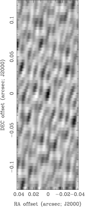
Figure 2.— Top: Typical u-v distribution with 1-min integration, corresponding to the 1665 MHz observation at an hour angle of 4 hours. Bottom: Typical one minute map produced with the 1665 MHz data.

Figure 3.— Top: Beam pattern as a function of right ascension and declination are given in the top and the bottom panel, respectively, for a data of one minute duration.

Figure 4.— Spectral line profile of W3(OH) corresponding to the one minute integration at 1665 MHz.

Numerous trial snap-shot images were made in order to determine the minimum time interval over which a successful and reliable image can be obtained. For these isolated strong sources ($\sim$10 Jy beam^-1), we find 1 minute as the shortest interval at which reliable images can be constructed with minimal problems of confusion (see below for a special case for the 1612 MHz line). In the top panel of Figure 2, we show the u-v coverage of a one minute interval at an hour angle of 4 hours for the 1665 MHz observation. To give an idea of the quality of map, we also show the map produced by a one minute observation in the bottom panel. Moreover, in the top and the bottom panels of Figure 3, we show the cross section of the beam along the right ascension and the declination directions, respectively. In order to demonstrate the signal to noise ratio of the detection of the spectral lines, we also show in Figure 4 the spectrum of the 1665 MHz line corresponding to the 1-min integration.

Out of the three sources given in Table 1, the sources at 1612 and 1720 MHz have been identified as Zeeman pairs. The corresponding longitudinal magnetic field strengths are given in the table from WGDa. At 1665 MHz, we do not observe a statistically significant shift between the line profiles in RR and LL channels. The integrated (over 12.5 hours) line profiles of these Zeeman components are shown in Figure 5.

Figure 5.— Integrated line profiles of W3(OH)corresponding to the three sources summarized in Table 1. Profiles with solid lines correspond to LL polarization, and the ones with ‘dashed’ lines correspond to the RR polarization.

The data analysis to identify and compute the line profiles was carried out using MIRIAD. Since some of the sources are clearly Zeeman pairs with velocity separations of the order of $\sim$1 km s^-1, (several freq channels), we carried out the analysis in both RR and LL polarization channels independently. The rationale for this procedure is that the intensity variations observed in the two polarizations may not necessarily be correlated even for small (¡ 0.1 to 0.2 km s^-1) velocity separations. The full 12.5 hour observation was used to constrain the source position and shape parameters (major and minor axis and PA). Then, we determined the flux density at 1 minute intervals, with the source position and the shape parameters held fixed. For this purpose, the MIRIAD task UVFIT was used. At the end of this step, we obtained line profiles every minute in RR and LL channels separately for all sources listed in Table 1. These profiles were arranged chronologically, forming a dynamic spectrum of intensity as a function of time and frequency (or velocity), for each source, in RR and LL separately.

For the 1612 MHz line, it was necessary to carry out a minor correction due to source confusion. The major 1612 MHz line has flux densities of 15 Jy (RR) and 4 Jy (LL). There is another source nearby (displaced by $-12$ mas in right ascension and $+1$ mas in declination) in the same velocity range. The flux density of this source is $\sim$1 Jy, which is about 10% of the more intense source. This weaker confusing source was imaged using the 12.5 hour observation; the mean flux density was subtracted from the entire u-v data base before the time series was constructed for the two major lines at RR and LL polarization. This method is based on the assumption that the time variation of the confusing source is minor compared to that of the brighter source based on the relative weakness of the confusing source.

4. Origin of flux density variations, and our model

Flux density variations with time scales of tens of minutes can be introduced by various effects that are independent of intrinsic variability. In order to explore the possibility that these maser sources exhibit intrinsic variability, it is essential to understand the nature of additional extrinsic sources of variability on relevant time scales.

First, any uncorrected instrumental gain variations in the receiver system will introduce apparent intensity variations. However, these changes will be correlated across spectral channels. In other words, we expect these changes to have a correlation bandwidth that is far wider than the typical spectral line widths of the maser sources of $\sim$0.5 km s^-1.

There is an effect that can potentially introduce flux density variability on short time scales. This effect arises from interstellar diffractive scintillations; two of the important parameters characterizing it are, namely, the decorrelation bandwidth ($\Delta\nu$), and the diffractive scintillation time scale ($T_{\rm dif}$). The latter ranges typically from minutes to hours. If the decorrelation bandwidth value is comparable to, or narrower than, the spectral line width of the maser source, i.e. less than a few channel widths or less than 0.2 to 0.4 km s${-1}$, then we would consider the temporal variations introduced by diffractive scintillations to be “narrowband”, and would expect significant differential variation within the line profile. In order to assess the situation correctly, we must estimate the expected value of the decorrelation bandwidth of diffractive scintillations along this sight-line.

Since these maser sources are spectral line emitters, measurements of the decorrelation bandwidth are often uncertain. However, the measured angular diameters of these sources provide an indirect estimate. The apparent angular width of many of the sources in W3(OH) are measurable in this data set, and is typically $\sim$3 mas (Palmer & Goss, Private communication). If we assume that this width is exclusively dominated by interstellar scatter broadening, i.e. the intrinsic angular size is significantly smaller than the apparent size, it is possible to calculate the expected relative time delay associated with the scattered rays with respect to the direct path (Gwinn et al. 1993; Deshpande & Ramachandran 1998). This effective time delay is identical to the characteristic temporal broadening scale ($\tau_{\rm sc}$) in the case of pulsar pulse profiles. At a distance of 2.0 kpc, and assuming that the scattering material is uniformly distributed along the line of sight, the delay is

$$\tau_{\rm sc}=\frac{D\;\theta_{H}^{2}}{16\;c\;\ln 2}\;\sim 4.5\;\;\mu{\rm s,}$$ (1)

where $D$ is the distance to the object, $\theta_{H}$ is the angular width of the source (full-width at half maximum), and $c$ is the speed of light. Since the decorrelation bandwidth and the effective time delay obey the following “reciprocal” relation,

$$2\pi\tau_{\rm sc}\;\delta\nu\;\approx\;1,$$ (2)

the value of the decorrelation bandwidth, $\delta\nu$ is then predicted to be $\sim$35 kHz. This is significantly greater than the typical line widths (1-2 kHz, or 0.2-0.4 km s^-1). Of course, this estimate is a worst-case estimate, where we have assumed that the observed width entirely arises from interstellar scattering. Even with this worst-case estimate, the expected differential variation within the spectral line profile as a function of time is only about $\sim$1% or less.

Apart from the above mentioned causes for intensity fluctuations, any additional observed variations may be assumed to be intrinsic to the maser source. Of course, we have no a priori knowledge about the nature of the intrinsic variations in OH masers. However, for the current analysis, we assume that the correlation bandwidth of any intrinsic variations is small enough to consider them as “narrowband”. That is, such variations in one channel would, in general, be uncorrelated with those in the other channels separated by our velocity/spectral resolution or more. There is an important reason for making this assumption. The possible intensity variations due to instrumental gain instability and interstellar diffractive scintillations are expected to be correlated across a velocity/spectral range much wider than the maser line widths, and hence can be treated as “broadband” variations, i.e. as modulations that are common to all the observed spectral/velocity channels. Therefore, in our analysis, we will be sensitive to only those intrinsic variations that are narrowband in nature, thereby clearly distinguishable from the instrumental and interstellar effects.

In order to quantify the observed variations, we have adopted the following procedure. We make a distinction between the different contributors to the observed flux density variance,

$$\sigma^{2}_{\rm obs}(v)\;=\;\sigma^{2}_{b}+\sigma^{2}_{i}(v)+\sigma^{2}_{n}(v).$$ (3)

The three terms in the above equation result from a “broadband” modulation, possibly intrinsic narrowband variability, and measurement uncertainty, respectively. For this purpose, we model the observed intensity $S_{obs}(t,v)$, i.e. a function of both time ($t$) and velocity ($v$) as

$$S_{\rm obs}(t,v)=S_{\rm ave}(v)\;[1+f_{b}(t)]\;[1+f_{v}(v,t)]\;+\;n(v,t),$$ (4)

where $f_{b}$ and $f_{v}$ are the zero-mean fractional variations that are of “broadband” and “narrowband” nature, respectively, and $n$ is the measurement noise, assumed to have zero mean. The function $S_{\rm ave}(v)$ refers to the average line-profile as a function of velocity. The time averaged cross-correlations between $f_{b}$, $f_{v}$ and $n$ are expected to be zero, i.e. they are assumed to be mutually uncorrelated. The parameter $f_{b}$, the “broadband” modulation, is independent of velocity (or frequency), and is therefore described as a function of time alone. Adopting the above formulation, the observed variance $\sigma^{2}_{\rm obs}$ in a given velocity channel can be expressed as

$$\sigma^{2}_{\rm obs}(v)=S^{2}_{\rm ave}(v)\;[\sigma^{2}_{c}+\sigma^{2}_{v}(v)]+\sigma^{2}_{n}(v),$$ (5)

where $\sigma_{c}$ and $\sigma_{v}(v)$ are the root-mean-square (RMS) fluctuations characterizing the fractional temporal variations $f_{b}$ and $f_{v}(v)$, respectively. $\sigma_{n}(v)$ is the RMS uncertainty in the measurements, which can be estimated in a straight-forward manner as $\sqrt{\sum e^{2}(v,t)/N}$ or $\sqrt{\langle e^{2}(v,t)\rangle_{t}}$. Here, $\langle x\rangle_{t}$ represents the average of “$x$” over time, and $e(v,t)$ (1-$\sigma$ error), is available for each of the $N$ (typically, 300-400) time samples in the dynamic spectrum $S_{\rm obs}(t,v)$ at a given velocity $v$. The $e(v,t)$ estimate for relevant channels also includes the contribution of the maser emission to the system noise. The desired quantity $\sigma_{v}(v)$, the modulation index associated with the “narrowband” variation (uncorrelated across velocity channels), can be estimated if $\sigma_{c}$ is known.

5. Correlation analysis to estimate “broadband” variation

In order to estimate and remove the possible contribution of any broadband variation (characterized by $\sigma_{c}$) from the observed variance, we examine the cross-correlations between the intensity fluctuations in all velocity-channel pairs. Auto-correlations are excluded since they, as seen from equation 5, are contaminated by the variance of measurement noise and narrowband fluctuations. Since $f_{b}$, $f_{v}$ and $n$ are mutually uncorrelated, the cross-correlation, expressed as “cross-variance”, between intensity fluctuations in any pair of channels (about their respective mean intensities) is given by

$$\sigma^{2}_{\rm obs}(v_{1},v_{2}) = \langle S_{\rm obs}(t,v_{1})\;S_{\rm obs}(t,v_{2})\rangle_{t}$$ (6)

$$= S_{\rm ave}(v_{1})\;S_{\rm ave}(v_{2})\;(\langle f_{b}(t)\;f_{b}(t)\rangle_{t}\;+$$

$$\;\langle f_{v}(v_{1},t)\;f_{v}(v_{2},t)\rangle_{t})\;+\;\langle n(v_{1},t)\;n(v_{2},t)\rangle_{t}$$

$$= S_{\rm ave}(v_{1})\;S_{\rm ave}(v_{2})\;\langle f_{b}(t)\;f_{b}(t)\rangle_{t}$$

$$= S_{\rm ave}(v_{1})\;S_{\rm ave}(v_{2})\;\sigma^{2}_{c},$$

where $v_{1}\neq v_{2}$. In a given velocity channel, the contribution due to any “broadband” intensity fluctuations, treated as an amplitude modulation, is expected to be proportional to the mean intensity associated with that channel. The cross-correlations between such fluctuations then will be proportional to the product of mean intensities of the corresponding pair of channels. The possible contribution from any “narrowband” fluctuation, $f_{v}(v,t)$, will also share this proportionality, but the associated cross-correlation is expected to have a zero-mean value. Similarly, the cross-variance of the measurement noise in any two different (and independent) velocity channels is also expected to be zero. Based on this assumption, we plot (as in the example shown in Figure 5) the cross-correlation $\sigma^{2}_{\rm obs}(v_{1},v_{2})$ (along the y-axis) against the associated product of mean intensities $S_{\rm ave}(v_{1})\;S_{\rm ave}(v_{2})$. From this plot an estimate of $\sigma^{2}_{c}$, or the slope of the expected linear dependence, can be derived. The velocity channels where the signal-to-noise ratio of the mean intensity $S_{\rm ave}(v)$ is less than 3 are excluded from this analysis. Naturally, the number of useful channels ($M$, typically about 5-6) based on this criterion is significantly reduced, but the resultant number of correlation pairs [$M(M-1)/2$] is large enough. The observed scatter about the linear dependence arises from the terms with $f_{v}$ and/or $n$, resulting in the uncertainty in the estimation of its slope. The two straight lines about the best-fit line, all passing through the origin, indicate the $\pm\sigma$ uncertainty in the slope. With $\sigma^{2}_{c}$ estimated in this manner, the “broadband” modulation contribution can now be removed from the observed variance.

In practice, any intrinsic fluctuation which may otherwise be uncorrelated between adjacent channels may contribute to some (positive) correlation due to the finite velocity resolution of the measured spectra (0.11 km s^-1 at 1665 MHz). Since such contributions will mimic correlations due to “broadband” modulation, these contributions can lead to an over-estimation of $\sigma^{2}_{c}$, and as a result, the contribution from “narrowband” fluctuations will be correspondingly underestimated. Any intrinsic fluctuation with a correlation bandwidth wider than the channel width will also be underestimated. If these effects are in fact significant, our estimates of the modulations index (or variance) associated with intrinsic variability can then be viewed as lower limits. As one possible measure against over-estimation of $\sigma^{2}_{c}$, we limit its value, if needed, such that $\sigma^{2}_{n}(v))$ is never negative (see Equation 5).

To assess the possible contamination due to these effects, as well as the robustness of the correlation procedure, we have repeated the analysis after normalization of each profile in the observed dynamic spectra with respect to (1) the velocity-averaged intensity, and (2) the intensity in a reference channel corresponding to the peak of the average profile. The estimates of $\sigma_{c}$ in these two cases are close to zero, suggesting that the above discussed contaminations are not significant. Also, the estimates of the intrinsic modulation are found to be consistent across the three methods, indicating that the estimate is not sensitive to whether or how the “broadband” variation was modified before applying the correlation procedure.

We have also examined the performance of the three methods when used separately. Although, they provide a consistent accounting (and removal) of the “broadband” modulation contribution, there are significant differences. Normalization with respect to the peak channel intensity is based on an implicit a priori expectation that the intrinsic variability in that reference channel is absent, and any observed variability is therefore only of “broadband” nature. Invalidity of this expectation can lead to a systematic over-estimation of the variance in the other channels, depending on the modulation index of the “narrowband” variation (including system noise) in the reference channel. However, for the channels adjacent to the reference channel sharing any common “narrowband” variability, the resultant variance would be underestimated. On the other hand, normalization based on the velocity-average intensity makes no assumption about absence of intrinsic variability in any particular channel, but does implicitly assume that the line-integral is intrinsically constant. Such an assumption has no physical justification. Hence, any “narrowband” variability, apart from its magnitude being underestimated, contaminates other channels with anti-correlated variations and a consequent increase in the variance. In both of these approaches, the corrected dynamic spectra are available, and can be examined using fluctuation spectral analysis for estimating the temporal scales of the remaining variability. In contrast, the correlation-based estimation and removal of the “broadband” contribution to the variance only produces time-averaged quantities, and hence any further temporal/spectral analysis can not be attempted. However, the correlation-based approach is the most unbiased in comparison with the two methods based on normalization. Therefore, for a determination of the variance associated with the “broad- and narrowband” variability, we have used the correlation-based procedure described above, and have only employed the normalization by intensity in the reference peak channel for the purposes of temporal/spectral analysis (e.g. §6).

Figure 6.— An example, based on W3OH 1665-MHz line (RR) data, to illustrate our procedure to estimate the possible contribution from “broadband” modulation. Here, we examine the cross-correlation between variations observed in every pair of channels versus the product of mean intensities corresponding to the respective channel pair. The observed trend is shown by the dashed line. Only those channels with their mean intensities having S/N greater than 3 are included. The slope of the expected linear dependence provides an estimate of $\sigma^{2}_{c}$ (see Equation 6), where $\sigma_{c}$ is the modulation index associated with the “broadband” modulation that is shared by all channels. The observed scatter about the linear dependence arises in general from any “narrowband” variations including the measurement noise. The middle of the three solid lines, always passing through the origin (0,0), indicates the best fit to the data, while the two other lines correspond to the $\pm 1-\sigma$ uncertainty in the slope.

The results from our variance analysis on all of the 6 data sets (consisting of dynamic spectra for RR & LL polarization for the sources in Table 1) are summarized in Figure 7, showing in each case the profiles of average line intensity ($S_{ave}$), as well as the standard deviations associated with the observed variability ($\sigma_{obs}(v)$), possible “broadband” modulation ($\sigma_{b}(v)$ = $\sigma_{c}S_{ave}(v)$) and the measurement uncertainties ($\sigma_{n}$). As already described and illustrated in Figure 6, the “broadband” modulation index $\sigma_{c}$ is estimated based on the cross-correlation analysis. The quantity $\sigma^{2}_{obs}-\sigma^{2}_{b}$, where the “broadband” modulation contribution is removed, represents the observed “narrowband” variance, which includes the nominally expected contribution $\sigma^{2}_{n}$ from the measurement noise. Also, we examine the ratio of the observed to the expected variances, $R=(\sigma^{2}_{obs}-\sigma^{2}_{b})/\sigma^{2}_{n}$, for any significant deviations from the expected value of unity. In other words, any statistically significant residual variance, i.e. $\sigma^{2}_{i}=\sigma^{2}_{obs}-\sigma^{2}_{b}-\sigma^{2}_{n}$, must then be “narrowband” in nature, and thus may be assumed to be intrinsic to the source. As another measure, we also compute the modulation index associated with the possible intrinsic “narrowband” variability, $\sigma_{v}=\sigma_{i}/S_{ave}$, where the signal-to-noise ratio of $S_{ave}$ estimate is three or more. The profiles of the ratio $R$ and $\sigma_{v}$ are also displayed in Figure 7.

A number of salient facts are evident from Figure 7. Firstly, statistically significant variations are indeed detected, even after accounting for the “broadband” modulation and measurement uncertainties. These variations, reflected by the excess variance at certain velocities, are “narrowband” in nature, and hence intrinsic to the source. Moreover, these variations are apparent at velocities away from the line peak, rather than at the peak. Within the statistical errors, the peaks do not appear to exhibit significant variations. The variations observed in the shoulders are detectable with signal-to-noise ratio of three or more.

Figure 7.— Results of the variance analysis of the dynamic spectral data on the sources listed in Table 1. The plots corresponding to the LL & RR polarization channels are shown on the left and the right columns, respectively, The top, middle and the bottom pairs show the results for the 1612, 1665 and 1720 MHz transitions, respectively. In each of the six plots, the top panel shows the average intensity profile (solid line), along with the profiles of standard deviations associated with the observed variance (dashed line), measurement noise (dotted line) and the “broadband” modulation (dot-dashed line), respectively. The latter is a scaled version of the average intensity profile, where the scale factor $\sigma_{c}$ is estimated using the cross-correlation procedure in §5. For clarity, all three profiles for the standard deviations are amplified by a factor of ten in this display. The middle panels display profiles of the ratio (R) of the observed “narrowband” variance to its expected value. The observed “narrowband” variance is simply the observed variance minus that associated with the “broadband” modulation, while the expected “narrowband” variance is that from the measurement noise ($\sigma^{2}_{e}$). The three curves correspond to the mean value of the ratio R, and with $\pm 1-\sigma$ deviations from this mean. The nominally expected values of R is unity within the indicated uncertainties, and any significant excess is interpreted as due to intrinsic “narrowband” variability. The modulation index (MI) associated with the latter, along with its $\pm 1-\sigma$ bounds are given in the bottom panel. The modulation index (MI) is computed as the ratio of the RMS fluctuations attributable to the intrinsic variability to the mean intensity $S_{ave}$, when both of them are significantly greater than zero. All of the estimates presented above are based on the data spanning 12.5 hours.

6. Velocity-Resolved fluctuation spectra, and time-scales of intrinsic variability

The basic data used here also are the dynamic spectra spanning 12.5 hour and obtained as chronologically arranged line profiles from one minute integrations. The aim of the fluctuation spectral analysis described below is twofold. The first is to examine the nature of the fluctuation spectra. Then, given the fluctuation spectra, to estimate the timescale of flux density variations arising from “narrowband” intrinsic variations. Thus it is essential to eliminate contribution from any “broadband” variations. To ensure this, each of the spectral profiles in the dynamic spectra is normalized with respective intensities in the reference channel defined by the peak in the average line profile. The justification for this normalization comes from the variance analysis (§5), where we concluded that the peak of the line profile does not exhibit any statistically significant “narrowband” variation. We can also rule out any overestimation of variability in other channels due to the normalization.

These “corrected” dynamic spectra for each of the sources form the input data for the velocity-resolved fluctuation spectral analysis. This analysis is very similar to the longitude-resolved fluctuation spectral analysis, a well known tool in pulsar emission studies (Backer 1973, Deshpande & Rankin 1999). Here, we compute fluctuation power spectrum for each of the velocity channels separately, where the single temporal sequence of intensities in a given channel is Fourier transformed and the power at each of the fluctuation frequencies computed. The results corresponding to all the velocity channels for a given line source are displayed together as a two-dimensional display of fluctuation power as a function of velocity and fluctuation frequency, along with a velocity-averaged power spectrum (see Figure 8).

Any statistically significant power observed in these fluctuation spectra can be interpreted as due to variability that is necessarily “narrowband”, and hence, intrinsic to the source. The following aspects are clearly evident from the spectra in Figure 8. The fluctuation power is generally higher in the line channels compared to those well away from the line emission, as would be expected from the measurement noise that will be proportional to the system temperature including the line intensity. Moreover, another thing that is apparent is that the fluctuation power toward lower frequencies is more than that at higher fluctuation frequencies. We examine also the spectrum computed by averaging the fluctuation spectra across the velocity channels. With the equivalent line width of only a couple of channels, given that the contribution of the line channels overwhelms in this average, the resultant spectrum has benefited only correspondingly from the averaging across velocity. Hence the ratio of the average power to the uncertainties (i.e. the signal-to-noise ratio) at any fluctuation frequency is rather small ($\sim$1.4), except when the fluctuation power in the line channels is small (e.g. as seen at the high fluctuation frequencies in some of the average spectra). Hence we do not consider the apparent fine spectral structure as significant, but rather examine and estimate the smooth trends across the spectrum, since they will have a much improved significance in accordance with the smoothing scale. The fluctuation power level at higher frequencies is consistently low, and corresponds largely to the measurement-noise contribution that is generally expected to be “white” (or uniform) in its spectral character. Thus the overall increase in the fluctuation power toward the lower frequency portion is significant in most cases (except for the 1665 line), where the power is typically about two to three times that at the higher frequency end of the average spectrum. The latter defines the reference noise floor, across which the RMS variation may be estimated and used to assess the significance of the contrast of fluctuation power levels between the two frequency ranges. For example, the increase in the average power toward lower frequencies for the 1612-MHz RR line is about seven times the RMS deviation in the power at the higher frequencies. This factor is somewhat lower for other lines/polarization channels, and is close to zero for the 1665 RR line.

We observe significant relative fluctuations up to a fluctuation frequency of $\sim 10^{-3}$ Hz, which corresponds to time scales of $\stackrel{{\scriptstyle>}}{{{}_{\sim}}}\,$15–20 min. Given that the normalization procedure has removed any extrinsic variability that is expected to be “broadband”, we associate this observed time scale with the intrinsic variability of the OH maser lines.

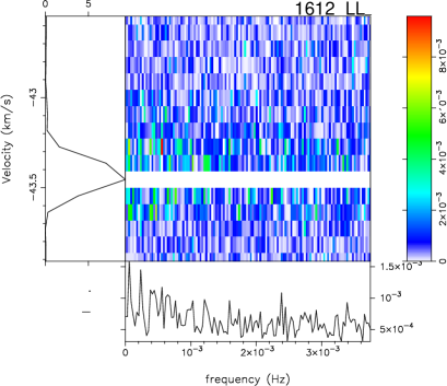
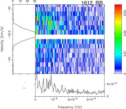
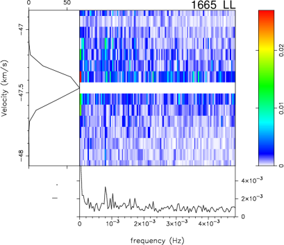
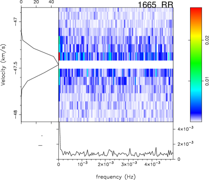
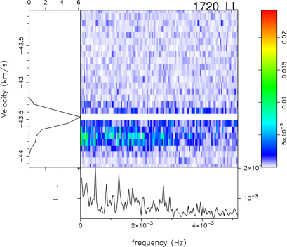
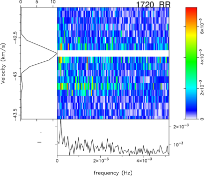
Figure 8.— Results of the Velocity-resolved fluctuation spectral analysis. The pair of plots from top to bottom correspond to the 1612, 1665 and 1720 MHz lines, respectively. In each of these pairs, the left and the right plots are for the LL, and RR polarization channels, respectively. Within each plot, the left side panels shows the average line profile (flux density in units of Jansky/beam) as a function of velocity obtained from the full observation. The central panel shows the velocity resolved fluctuation spectra, where each horizontal row is the power spectrum of the time series from the corresponding velocity channel. Each time series is normalized with respect to the time series for the reference peak channel. Naturally, this results in a null spectrum for the reference channels. As the color bar shows, red corresponds to the maximum power, and white corresponds to zero power. The bottom panel gives the velocity-averaged fluctuation spectrum. In most cases, significant fluctuation power is apparent at lower frequencies in comparison with the noise floor at the higher frequency end of the spectra. As discussed in the main text, the observed “narrowband” variability on time scales of 15-20 minutes or longer is to be understood as intrinsic to the maser sources.

7. Discussion and Summary

In this work, we have conclusively demonstrated the presence of “narrowband” intrinsic variations in these W3(OH) maser sources. These variations seem to have a typical time scale of about 15-20 minutes or longer, indicating that the faster time scale may correspond to the light travel time of the maser pumping column.

A very important aspect, which is worth stating again, is that the observed intrinsic variations that are clearly separable from other contaminants are necessarily “narrowband” in nature. All the other variations such as the instrumental gain variations and the interstellar diffractive scintillation, although their time scales may be of the order of a few tens of minutes, are distinguishable from the intrinsic variabilities, mainly because of their broad correlation bandwidth. The expected differential fluctuation within the line profile due to interstellar scintillation is only of the order of $\sim$0.5%, much smaller than the observed intrinsic variability, whose magnitude was as much as 100% (modulation index), in the “tail” portions of the spectral lines.

There is one source of systematic narrowband error that could have potentially influenced our conclusions. In our VLBI measurements, if the Earth’s motion were not correctly compensated for, certain systematic but spurious temporal variations in the line profiles would be induced due to differential Doppler shift. However, we would then expect the variations seen on the two sides of the line profile peak to be anti-correlated. We have examined carefully the relevant cross-correlations, and do not find any statistically significant signature such an anti-correlation, clearly indicating that our data are free of such artefact.

An important aspect of these maser sources is that their typical measured angular diameter is $\sim$3 mas. With the distance to the star forming region of 2 kpc, this corresponds to a transverse distance scale of $\sim$ 6 AU. As we have seen from Figure 8, the fluctuation frequencies seen in the spectra are $\raisebox{-1.29167pt}{\mbox{$\stackrel{{\scriptstyle<}}{{{}_{\sim}}}\,$}}10^{-3}$ Hz (fluctuation time scale, $T_{f}\sim 1000$ s or longer). If indeed this time scale reflects the dimension of the source based on light travel time arguments, then the implied longitudinal spatial scale of the maser column would be 2–3 AU. It is important to note that the apparent transverse spatial dimension of the source as measured from the angular size is comparable to its longitudinal dimension implied by the fluctuation timescale, even though there seems to be no a priori basis for the comparison, let alone the agreement. However, if indeed these orthogonal dimensions of the source are expected to comparable, it would imply that the VLBA observations may have actually resolved the intrinsic source size of the OH masers in W3(OH). Then the possible contribution of angular broadening caused by interstellar scattering to the apparent size of the source is minimal. This also implies that the expected decorrelation bandwidth of interstellar scintillation may be much wider than 100 kHz, further reinforcing the validity of our assumptions. However, if the scatterer is closer to the source instead of the midway location which is implicit in equation 1, the decorrelation bandwidth would be correspondingly narrower. We assess whether that may be the case, based on the two important estimates we have at hand, namely the measured upper-limit for scatter broadening $\theta_{H}$ and the observed time scales (say, $T_{\rm dif}$) of the narrow-band variability, if due to ISM, since that is our concern. How far are we from the naive assumption of uniform scatterer (or a strong scatterer mid-way) will be reflected in both of these parameters, which depend differently on the relative location of the scatterer (see for example, eq. 3 and 8 of Deshpande & Ramachandran 1998). If $D_{s}$ & $D$ are the distances of the scatterer and of the observer, respectively, as measured from the source, it is easy estimate an upper limit to ($D/D_{s}$ -1) using relevant expressions, and assuming that the observed time-scales are 1000 s or longer, & a wavelength of 18 cm. We find that ($D/D_{s}$ -1) should be less than or equal to $20/(\theta_{H}V_{ism})$, where the scatter broadening $\theta_{H}$ is in mas, and the ISM velocity $V_{ism}$ is in km s^-1. A value of 3 mas for $\theta_{H}$ implies $(D/D_{s}-1)\leq 6.6/V_{ism}$. Noting that $V_{ism}$ will have the same lever-arm factor as source velocity does, and considering typical values of $V_{ism}$, we conclude that $(D/D_{s}-1)$ is close to unity, if not smaller. Hence, the decorrelation bandwidth that we estimate naively is most likely an under-estimate, given the above and that $\theta_{H}$ may already be an over-estimate of the scatter broadening.

As already mentioned in the introduction, variability of astrophysical masers on longer time scales — weeks to months — observed before by several investigators, may be due to changes in the number density of relevant molecules or physical conditions in the maser column. On the other hand, very short time scale rapid variations have also been seen. Salem & Middleton (1978) suggest a model in which a sudden onset of a pumping mechanism can cause rapid quasi-periodic fluctuations in the observed flux density, and predict fluctuations with time scales of a day or so, with $\sim$25% modulation index. These fluctuations may either correspond to propagation of a radiative or a collisional disturbance. In the former case the disturbance travels with the speed of light, and in the latter with a typical speed of $\sim$10 km s^-1 or so. For radiative propagation of disturbance, with the typical flux density of the observed lines, the brightness temperature comes to $\sim 10^{10}$K. For a collisional disturbance, the source dimension is only $T_{f}\times 10$ km s^-1 $\approx 10^{7}$ meters (angular diameter of $\sim$0.1 $\mu$arcsec). This corresponds to a brightness temperature of $\sim 10^{20}$K (see also Clegg & Cordes 1991). In the latter case, since the implied intrinsic angular diameter is only $\sim$1$\mu$arcsec, the observed angular diameter is predominantly due to interstellar scattering. For an object at 2.2 kpc (distance of W3(OH) complex), a scatter broadening of 2–3 arcsec seems to be very large at the 18-cm wavelength. VLBI observations of several nearby (distance less than 2–3 kpc) pulsars at 327 MHz have shown a broadening of 10–20 mas, with an exception of the Vela pulsar, PSR B0833–45 (Gwinn, Bartel & Cordes 1993). In the case of Vela, the excess angular broadening is due to the presence of strong scattering screen (Deshpande & Ramachandran 1998). Assuming a Kolmogorov density irregularity spectrum, with the wavelength dependence of $\lambda^{2.2}$, the expected angular broadening is only $<0.5$ mas at 1665 MHz. Based on these considerations, we argue against any significant over-estimation of the source size of W3(OH) due to scatter broadening.

It has been suggested by Elitzur (1991) that short time scale intensity variations can be produced by variations in the maser level population at small length scales. These fluctuations produced in the unsaturated medium of the maser core give rise to the spectrum of flux density variability observed. In our case, with the length scale of 2-3 AU (derived based on the light travel time arguments) represents an average “seed” length for such a fluctuation. This suggestion may well be the reason for the short time scale fluctuations that we have observed.

As mentioned earlier, the longitudinal dimension 2-3 AU estimated from the observed time scales of intrinsic variability compares well with the transverse spatial dimension of 6 AU estimated assuming that the apparent angular size to be approximately the intrinsic size of the source. However, for estimating brightness temperature the source we will use only its transverse size. A typical observed flux density of some 10 Jy at the line peaks (e.g. for 1612/1720 lines), implies a peak brightness temperature of $\sim 2\times 10^{13}$ K. A five times higher value, i.e. $\sim 10^{14}$ K, is implied by the correspondingly brighter peaks of the 1665 lines.

The intrinsic intensity variations that we observe are particularly confined to the “shoulders” of the lines and away from the line peak (see Figure 7). The peak of the line profiles does not exhibit any statistically significant variation, in all of the six data sets. This behavior is not at all surprising if the peak of these line emissions corresponds to “saturated” maser action, and the rest of the line profile exhibits unsaturated emission. In any case, the absence of any intrinsic variability at the line peak enables use of the corresponding channel intensities to calibrate out any “broadband” variations from the dynamic spectrum.

Another interesting aspect apparent from the results in Figure 7 is that the statistically significant narrowband variations that we observe at the raising and falling edges of the line profiles are not identical between the Zeeman pairs (RR and LL components). For instance, the difference between the modulation indices of the two Zeeman components of 1720 MHz lines is clearly seen to be several times the root mean square noise level. The physical reason for this behavior needs to be explored. Given the birefringent nature of the medium close to or at the origin of the radiation, as well as interstellar propagation medium, effects of refraction on the apparent visibility of the two Zeeman components remain to be explored.

To summarize, we list our main conclusions as follows.

• The combination of our cross-correlation procedure and the variance analysis provides an effective tool for estimation and elimination of the “broadband” contribution from instrumental effects and the interstellar diffractive scintillation, and thus for identifying variations that are intrinsic and “narrowband” in nature.

• Significant intrinsic “narrowband” variability is observed over most regions of the line profiles except at and about the line peak, suggesting “saturated” maser emission at the peak.

• The velocity-resolved fluctuation spectra reveal that the time scales of the significant intrinsic variability are 15-20 minutes or longer.

• Based on light travel time argument, the intrinsic variability time scale implies a longitudinal spatial scale of the maser column to be about 2-3 AU.

• The apparent angular sizes of the sources are unlikely to be significantly affected by interstellar scattering. The implied transverse size of the source is comparable to its longitudinal dimension.

• The peak brightness temperatures for the maser sources range between $\sim 2\times 10^{13}$ and $\sim 10^{14}$ K.

References

- (1) Backer, D. C. 1973, ApJ, 182, 245
- (2) Burke, B. F. et al. 1968, AJ, 73, S168
- (3) Clegg, A. W. & Cordes, J. M. 1991, ApJ, 374, 150
- (4) Coles, W. A., Rumsey, V. H. & Welch, W. J. 1968, ApJ, 154, L61
- (5) Desai, K. M., Gwinn, C. R. & Diamond, P. J. 1994, Nature, 372, 754
- (6) Deshpande, A. A. & Ramachandran, R. 1998, MNRAS, 300, 577
- (7) Deshpande, A. A. & Rankin, J. M. 1999, ApJ, 524, 1008
- (8) Elitzur, M. 1991, ApJ, 370, 45
- (9) Evans, N. J., Hills, R. E., Rydbeck, O. E. H. & Kollberg, E. 1972, BAAS, 4, 225
- (10) Fish, V. L., Reid, M. J., Argon, A. L., & Zheng, X.-W. 2005, ApJS, 160, 220
- (11) Fish, V. L., & Reid, M. J. 2006, ApJS, in press (astro-ph/0601560)
- (12) Gray, M. D., Cohen, R. J., Richards, A. M. S., Yates, J. A. & Field, D. 2001, MNRAS, 324, 643
- (13) Gruber, G. M. & de Jager, G. 1976, A&A, 50, 313
- (14) Gwinn, C. R., Bartel, N. & Cordes, J. M. 1993, ApJ, 410, 673
- (15) Gwinn, C. R., Moran, J. M. & Reid, M. J., Schneps, M. H. 1988, ApJ, 330, 817
- (16) Hachisuka, K., Brunthaler, A., Hagiwara, Y., Menten, K. M., Imai, H., Miyoshi, M. & Sasao, T. 2004, astro-ph/0409343
- (17) Rickard, L. J., Zuckerman, B. & Palmer, P. 1975, ApJ, 200, 6
- (18) Salem, M. & Middleton, M. S. 1978, MNRAS, 183, 491
- (19) Schwartz, P. R., Harvey, P. M. & Barrett, A. H. 1974, ApJ, 187, 491
- (20) Wright, M. M., Gray, M. D. & Diamond, P. J. 2004a, MNRAS, 350, 1253
- (21) Wright, M. M., Gray, M. D. & Diamond, P. J. 2004b, MNRAS, 350, 1272
- (22) Wright, M. M., Gray, M. D. & Diamond, P. J. 2005, MNRAS, 357, 800
- (23) Xu, Y., Reid, M. J., Zheng, X. W. & Menten, K. M. 2006, Science, 311, 54
- (24) Zuckerman, B., Yen, J. L., Gottlieb, C. A. & Palmer, P. 1972, ApJ, 177, 59