A relativistic model of the radio jets in 3C 296

Abstract

We present new, deep 8.5-GHz VLA observations of the nearby, low-luminosity radio galaxy 3C 296 at resolutions from 0.25 to 5.5 arcsec. These show the intensity and polarization structures of the twin radio jets in detail. We derive the spectral-index distribution using lower-frequency VLA observations and show that the flatter-spectrum jets are surrounded by a sheath of steeper-spectrum diffuse emission. We also show images of Faraday rotation measure and depolarization and derive the apparent magnetic-field structure. We apply our intrinsically symmetrical, decelerating relativistic jet model to the new observations. An optimized model accurately fits the data in both total intensity and linear polarization. We infer that the jets are inclined by $58^{\circ}$ to the line of sight. Their outer isophotes flare to a half-opening angle of 26^∘ and then recollimate to form a conical flow beyond 16 kpc from the nucleus. On-axis, they decelerate from a (poorly-constrained) initial velocity $\beta=v/c\approx 0.8$ to $\beta\approx 0.4$ around 5 kpc from the nucleus, the velocity thereafter remaining constant. The speed at the edge of the jet is low everywhere. The longitudinal profile of proper emissivity has three principal power-law sections: an inner region (0 – 1.8 kpc), where the jets are faint, a bright region (1.8 – 8.9 kpc) and an outer region with a flatter slope. The emission is centre-brightened. Our observations rule out a globally-ordered, helical magnetic-field configuration. Instead, we model the field as random on small scales but anisotropic, with toroidal and longitudinal components only. The ratio of longitudinal to toroidal field falls with distance along the jet, qualitatively but not quantitatively as expected from flux freezing, so that the field is predominantly toroidal far from the nucleus. The toroidal component is relatively stronger at the edges of the jet. A simple adiabatic model fits the emissivity evolution only in the outer region after the jets have decelerated and recollimated; closer to the nucleus, it predicts far too steep an emissivity decline with distance. We also interpret the morphological differences between brightness enhancements (“arcs”) in the main and counter-jets as an effect of relativistic aberration.

1 Introduction

The case that the jets in low-luminosity, FR I radio galaxies (Fanaroff & Riley, 1974) are initially relativistic and decelerate to sub-relativistic speeds on kiloparsec scales rests on several independent lines of evidence, as follows.

1. Proper motions corresponding to speeds comparable with or exceeding $c$ have been observed directly on pc and kpc scales in FR I jets (Giovannini et al., 2001; Biretta, Zhou & Owen, 1995; Hardcastle et al., 2003).

2. FR I sources must be the side-on counterparts of at least a subset of the BL Lac population, in which evidence for bulk relativistic flow on pc scales is well established (e.g. Urry & Padovani 1995).

3. FR I jets show side-to-side asymmetries which decrease with distance from the nucleus, most naturally explained by Doppler beaming of emission from an intrinsically symmetrical, decelerating, relativistic flow (Laing et al., 1999), in which case the brighter jet is approaching us. There is continuity of sidedness from pc to kpc scales and superluminal motion, if observed, is in the brighter jet.

4. The lobe containing the brighter jet is less depolarized than the counter-jet lobe, consistent with Faraday rotation in the surrounding halo of hot plasma if the brighter jet is approaching (Laing, 1988; Morganti et al., 1997).

5. Theoretical work has demonstrated that initially relativistic jets can decelerate from relativistic to sub-relativistic speeds without disruption provided that they are not too powerful, the surrounding halo of hot plasma providing a pressure gradient large enough to recollimate them (Phinney, 1983; Bicknell, 1994; Komissarov, 1994; Bowman, Leahy & Komissarov, 1996).

We have developed a method of modelling jets on the assumption that they are intrinsically symmetrical, axisymmetric, relativistic, decelerating flows. By fitting to deep radio images in total intensity and linear polarization, we can determine the three-dimensional variations of velocity, emissivity and magnetic-field ordering. We first applied the technique to the jets in the radio galaxy 3C 31 (Laing & Bridle, 2002a, LB). With minor revisions, the same method proved capable of modelling the jets in B2 0326+39 and B2 1553+24 (Canvin & Laing, 2004, CL) and in the giant radio galaxy NGC 315 (Canvin et al., 2005, CLBC). We used the derived velocity field for 3C 31, together with Chandra observations of the hot plasma surrounding the parent galaxy, to derive the run of pressure, density, Mach number and entrainment rate along its jets via a conservation-law analysis (Laing & Bridle, 2002b). We also examined adiabatic models for 3C 31 in detail (Laing & Bridle, 2004).

We now present a model for the jets in 3C 296, derived by fitting to new, sensitive VLA observations at 8.5 GHz. In Section 2, we introduce 3C 296 and summarize our VLA observations and their reduction. Images of the source at a variety of resolutions are presented in Section 3, where we also describe the distributions of spectral index, rotation measure and apparent magnetic field derived by combining our new images with lower-frequency data from the VLA archive. We briefly recapitulate our modelling technique in Section 4 and compare the observed and model brightness and polarization distributions in Section 5. The derived geometry, velocity, emissivity and field distributions are presented in Section 6. We compare the result of model fitting for the five sources we have studied so far in Section 7 and summarize our results in Section 8.

We adopt a concordance cosmology with Hubble constant, $H_{0}$ = 70 $\rm{km\,s^{-1}\,Mpc^{-1}}$, $\Omega_{\Lambda}=0.7$ and $\Omega_{M}=0.3$. Spectral index, $\alpha$, is defined in the sense $S(\nu)\propto\nu^{-\alpha}$ and we use the notations $P=(Q^{2}+U^{2})^{1/2}$ for polarized intensity and $p=P/I$ for the degree of linear polarization. We also define $\beta=v/c$, where $v$ is the flow velocity. $\Gamma=(1-\beta^{2})^{-1/2}$ is the bulk Lorentz factor and $\theta$ is the angle between the jet axis and the line of sight.

2 Observations and images

2.1 3C 296

For our modelling technique to work, both radio jets must be detectable at high signal-to-noise ratio in linear polarization as well as total intensity, separable from any surrounding lobe emission, straight and antiparallel. 3C 296 satisfies all of these criteria, although the lobe emission is relatively brighter than in the other sources we have studied. This is a potential source of error, as we shall discuss.

3C 296 was first imaged at 1.4 and 2.7 GHz by Birkinshaw, Laing & Peacock (1981). VLA observations showing the large-scale structure at 1.5 GHz and the inner jets at 8.5 GHz were presented by Leahy & Perley (1991) and Hardcastle et al. (1997) respectively.

The large-scale radio structure of 3C 296 has two radio lobes with well-defined outer boundaries and weak diffuse “bridge” emission around much of the path of both jets, at least in projection (Leahy & Perley, 1991). 3C 296 is therefore more typical of a “bridged twin-jet” FR I structure (Laing, 1996) than the “tailed twin-jet” type exemplified by 3C 31 and other sources we have studied so far. Parma et al. (1996) point out that the “lobed, bridged” FR I population is more abundant in a complete sample of low-luminosity radio galaxies than the “plumed, tailed” population. It is therefore particularly interesting to compare the inferred properties of the jets in 3C 296 with those of the sources we have modelled previously. Of the two lobes, that containing the counter-jet depolarizes more rapidly with decreasing frequency between 1.7 and 0.6 GHz (Garrington, Holmes & Saikia, 1996), consistent with the idea that it is further away from us.

The parsec-scale structure, imaged by Giovannini et al. (2005), is two sided, but brighter on the same side as the kpc-scale jet emission. Non-thermal X-ray and ultraviolet emission have been detected from the brighter jet (Hardcastle et al., 2005) and the nucleus (Chiaberge, Capetti & Celotti, 1999; Hardcastle et al., 2005). The source is associated with the giant elliptical galaxy NGC 5532 ($z=0.02470\pm 0.00007$), the central, dominant member of a small group (Miller et al., 2002). The linear scale is 0.498 kpc arcsec^-1 for our adopted cosmology. The galaxy has a slightly warped nuclear dust ellipse in PA $163^{\circ}\pm 4^{\circ}$ with an inclination of $73^{\circ}\pm 4^{\circ}$ assuming intrinsic circularity (Martel et al., 1999; de Koff et al., 2000; Verdoes Kleijn & de Zeeuw, 2005, parameters are taken from the last reference). X-ray emission from hot plasma associated with the galaxy was detected by ROSAT and imaged by Chandra (Miller et al., 1999; Hardcastle & Worrall, 1999; Hardcastle et al., 2005).

2.2 Observations

New, deep VLA observations of 3C 296 at 8.5 GHz are presented here. We were interested primarily in the inner jets, and therefore used a single pointing centre at the position of the nucleus and the maximum bandwidth (50 MHz) in each of two adjacent frequency channels. In order to cover the full range of spatial scales in the jets at high resolution, we observed in all four VLA configurations. We combined our new datasets with the shorter observations described by Hardcastle et al. (1997), which were taken with the same array configurations, centre frequency and bandwidth.

In order to correct the observed ${\bf E}$-vector position angles at 8.5 GHz for the effects of Faraday rotation and to estimate the spectrum of the source, we also reprocessed earlier observations at 4.9 GHz and 1.4 – 1.5 GHz (L-band). The 4.9-GHz data were taken in the A configuration. At L-band, we used two A-configuration observations (the later one also from Hardcastle et al. 1997) and the combined B, C and D-configuration dataset from Leahy & Perley (1991). A journal of observations is given in Table 1.

Table 1: Journal of VLA observations. $\nu$ and $\Delta\nu$ are the centre frequencies and bandwidth, respectively, for the one or two frequency channels observed and t is the on-source integration time scaled to an array with all 27 antennas operational. References to previous publications using the same data: 1 Hardcastle et al. (1997), 2 Leahy & Perley (1991).

Config-	Date	$\nu$	$\Delta\nu$	t	Ref
uration		(GHz)	(MHz)	(min)
A	1995 Jul 24	8.4351, 8.4851	50	123	1
B	1995 Nov 27	8.4351, 8.4851	50	110	1
C	1994 Nov 11	8.4351, 8.4851	50	47	1
D	1995 Mar 06	8.4351, 8.4851	50	30	1
A	2004 Dec 12	8.4351, 8.4851	50	250
A	2004 Dec 13	8.4351, 8.4851	50	253
B	2005 Apr 21	8.4351, 8.4851	50	250
B	2005 Apr 23	8.4351, 8.4851	50	264
C	2005 Jul 14	8.4351, 8.4851	50	249
D	2005 Nov 27	8.4351, 8.4851	50	98
A	1981 Feb 13	4.8851	50	130
A	1981 Feb 13	1.40675	12.5	125
A	1995 Jul 24	1.3851, 1.4649	50	45	1
B	1987 Dec 08	1.4524, 1.5024	25	60	2
C	1988 Mar 10	1.4524, 1.5024	25	50	2
D	1988 Oct 7	1.4524, 1.5024	25	80	2

2.3 Data reduction

2.3.1 8.5 GHz observations

All of the 8.5-GHz datasets were calibrated using standard procedures in the aips package. 3C 286 was observed as a primary amplitude calibrator and to set the phase difference between right and left circular polarizations; J1415+133 was used as a secondary phase and amplitude calibrator and to determine the instrumental polarization. After initial calibration, the 1994-5 data were precessed to equinox J2000 and shifted to the phase centre of the new observations. All three A-configuration datasets were then imaged to determine a best estimate for the position of the core (RA 14 16 52.951; Dec. 10 48 26.696; J2000) and then self-calibrated, starting with a phase-only solution for a point-source model at the core position and performing one further phase and one amplitude-and-phase iteration with clean models. The core varied significantly between observations, so we added a point source at the position of the peak to the 1995 dataset to equalize the core flux densities. We then combined the three A-configuration datasets and performed one further iteration of phase self-calibration. The B-configuration datasets were initially phase self-calibrated using the A-configuration model. After further iterations of self-calibration and adjustment of the core flux density, they were concatenated with the A-configuration dataset. The process was continued to add the C- and D-configuration datasets, with relative weights chosen to maintain a resolution of 0.25 arcsec for images from the final combination.

The off-source noise levels for the final $I$ images ($\approx 4\mu$Jy beam^-1 rms at full resolution) are close to the limits set by thermal noise, although there are slight residual artefacts within a pair of triangles centred on the core and defined by position angles $\pm 15^{\circ}$. These do not affect the jet emission, and the maximum increase in noise level is in any case only to $\approx 6\mu$Jy beam^-1 rms at full resolution. $I$ images were made using clean and maximum-entropy deconvolution, the latter being convolved with the same Gaussian beam used to restore the clean images. Differences between the two deconvolutions were very subtle. As usual, the maximum-entropy method gave smoother images, avoiding the mottled appearance produced by clean in regions of uniform surface brightness. On the other hand, the clean images had slightly lower off-source noise levels, significantly lower (and effectively negligible) zero-level offsets, and improved fidelity in regions with high brightness gradients. The differences between the two methods are sufficiently small that none of our quantitative conclusions is affected by choice of method. We have used the clean deconvolutions for all of the modelling described in Sections 4 – 6, but have generally preferred the maximum entropy images for the grey-scale displays in Section 3. All $Q$ and $U$ images were cleaned.

We made $I$, $Q$ and $U$ images at standard resolutions of 5.5, 1.5, 0.75 and 0.25 arcsec FWHM. All images were corrected for the primary-beam response during or after deconvolution, so the noise levels (listed in Table 2) strictly apply only in the centre of the field. The total flux density determined by integrating over a clean image at 5.5 arcsec resolution is 1.31 Jy (with an estimated error of 0.04 Jy due to calibration uncertainties alone), compared with an expected value of $1.20\pm 0.06$ Jy, interpolated between single-dish measurements at 10.7 and 5.0 GHz (Laing & Peacock, 1980). At least in the low-resolution images, we have therefore recovered the total flux density of the source, despite the marginal spatial sampling (Table 2).

Table 2: Resolutions and noise levels for the images used in this paper. $\sigma_{I}$ is the off-source noise level on the $I$ image; $\sigma_{P}$ the average of the noise levels for $Q$ and $U$. M and C denote maximum-entropy and CLEAN $I$ deconvolutions. All noise levels were determined before correction for the primary beam response and larger values are appropriate at significant distances from the field centre. The approximate maximum scale of structure imaged reliably is also given (Taylor, Ulvestad & Perley, 2004). Note that the 1.5-arcsec L-band image includes A-configuration data at 1.41 GHz and BCD configuration data at 1.45/1.50 GHz (see text).

FWHM	Freq	Config-	rms noise level			Max
(arcsec)	GHz	urations	[$\mu$Jy beam-1]			scale
			$\sigma_{I}$		$\sigma_{P}$	arcsec
			M	C
5.5	8.4601	ABCD	$-$	15	8.8	180
5.5	1.5024	BCD	$-$	40	40	900
5.5	1.4524	BCD	$-$	90	35	900
5.5	1.4774	BCD	$-$	38	$-$	900
1.5	8.4601	ABCD	9.5	9.1	4.8	180
1.5	1.3851	A	$-$	$-$	37	40
1.5	1.4649	A	$-$	$-$	35	40
1.5	1.40675	ABCD	27	$-$	$-$	900
0.75	8.4601	ABCD	4.3	4.2	4.1	180
0.40	8.4601	ABCD	$-$	4.2	$-$	180
0.40	4.8851	A	$-$	33	$-$	10
0.25	8.4601	ABCD	4.9	3.6	4.5	180

2.3.2 4.9 and 1.4–1.5 GHz observations

For the B, C and D-configuration observations at 1.45 and 1.50 GHz, we started from the combined dataset described by Leahy & Perley (1991). We imaged a significant fraction of the primary beam using a faceting procedure in order to minimize errors due to non-coplanar baselines and confusion, using the resulting clean model as the input for a further iteration of phase-only self-calibration. This led to a significant improvement in off-source noise level compared with the values obtained by Leahy & Perley 1991 using earlier algorithms. The noise level in $I$ is much larger at 1.45 GHz than at 1.50 GHz, probably as a result of interference; the $Q$ and $U$ images in the two frequency channels have similar noise levels, however. We used both single-frequency and combined images at 5.5-arcsec resolution; the former for polarization and the latter for spectral index. The reason was that the variation of Faraday rotation across the structure turned out to be large enough that the ${\bf E}$-vector position angle difference between the two frequency channels changed significantly across the structure (Section 3.3), whereas the variations of spectral index did not lead to detectable differences between the $I$ images in the two channels (Section 3.2).

The A-configuration observations at 1.39, 1.41, 1.46 and 4.9 GHz were calibrated, self-calibrated and imaged using standard methods. The 1.41-GHz A configuration dataset had better spatial coverage (in multiple separated snapshots) but poorer sensitivity compared with the later short observations at 1.39/1.46 GHz. We were able to make a satisfactory multi-configuration $I$ image at 1.5 arcsec resolution using the 1.41-GHz dataset together with the 1.45/1.50-GHz BCD configuration combination. No core variability was apparent between observations. The frequency difference is sufficiently small that there should be no significant effects on the spectral index image of the jets (see Section 3.2). The clean deconvolution of this combined ABCD configuration L-band image image had significant artefacts, but the maximum-entropy image at this resolution was adequate, at least in the area of the jets. In order to determine rotation measures, however, the individual IFs were kept separate (exactly as in the lower-resolution case) and we therefore made $Q$ and $U$ images from the individual A-configuration datasets.

The A-configuration image at 4.9 GHz shows only the innermost regions of the jets. No significant polarization is detected and we use it only to estimate the spectral index of the jets at high resolution.

Details of the images are again given in Table 2.

3 Total intensity, spectrum, Faraday rotation and apparent magnetic field

3.1 Total-intensity images

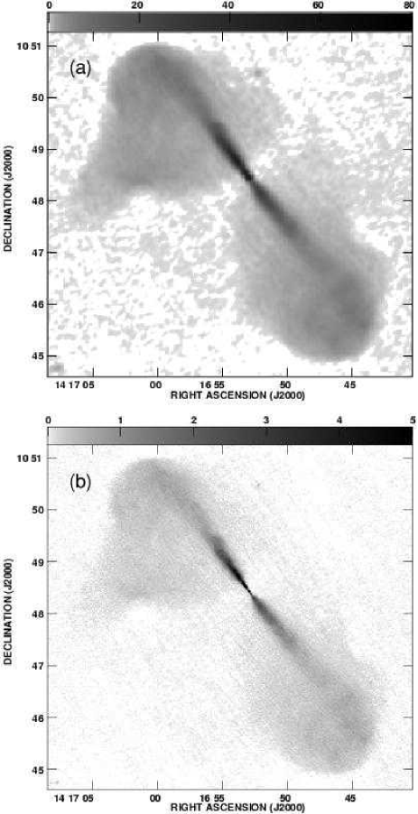
Figure 1: Grey-scales of total intensity. A square-root transfer function has been used to emphasise the low-brightness emission. (a) 1.48-GHz BCD CLEAN image at 5.5-arcsec FWHM resolution. The grey-scale range, 0 – 80 mJy (beam area)^-1, is marked by the labelled wedge. (b) L-band ABCD maximum entropy image at 1.5-arcsec FWHM resolution from a combination of 1.41 and 1.48-GHz datasets. The grey-scale range is 0 – 5 mJy beam^-1. The areas covered by the two panels are identical.

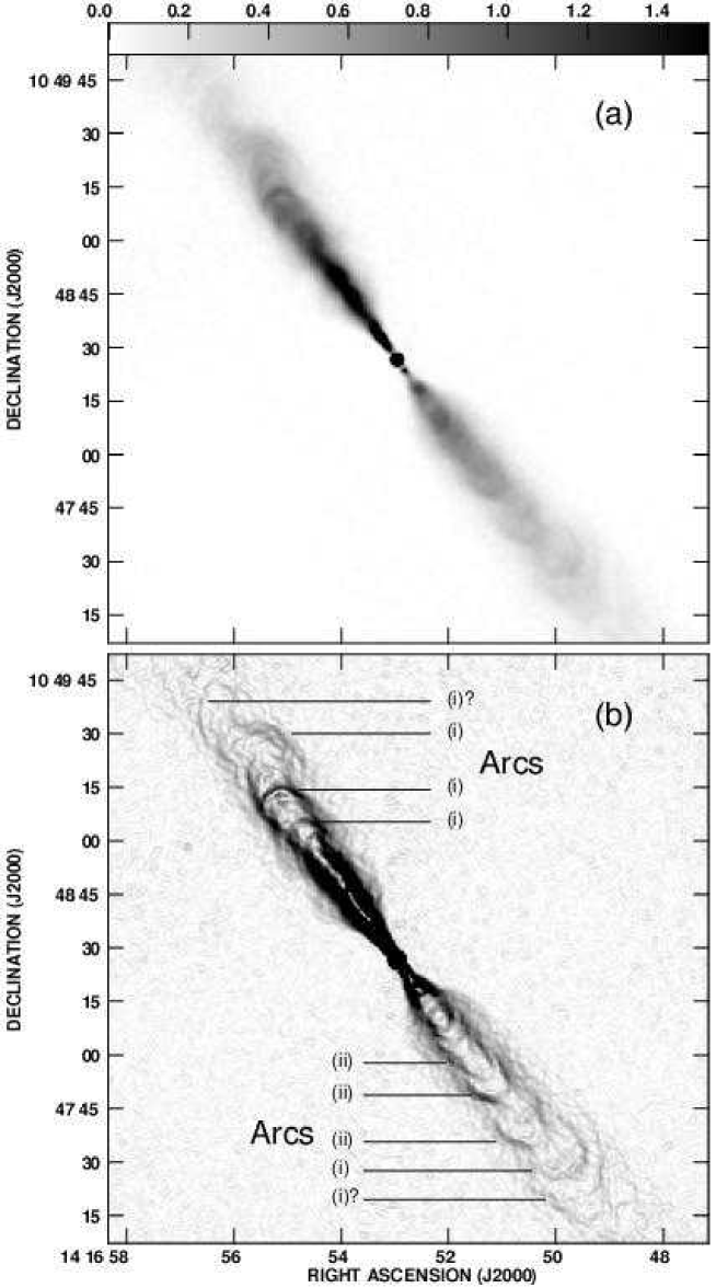
Figure 2: (a) Grey-scale of total intensity for a maximum-entropy image of the jets of 3C 296 at 8.5 GHz. The resolution is 1.5 arcsec FWHM and the grey-scale range is 0 – 1.5 mJy beam^-1. (b) Grey-scale of a Sobel-filtered version of this image. Narrow features in the brightness distribution (“arcs”) are marked with their types as defined in Section 3.1.

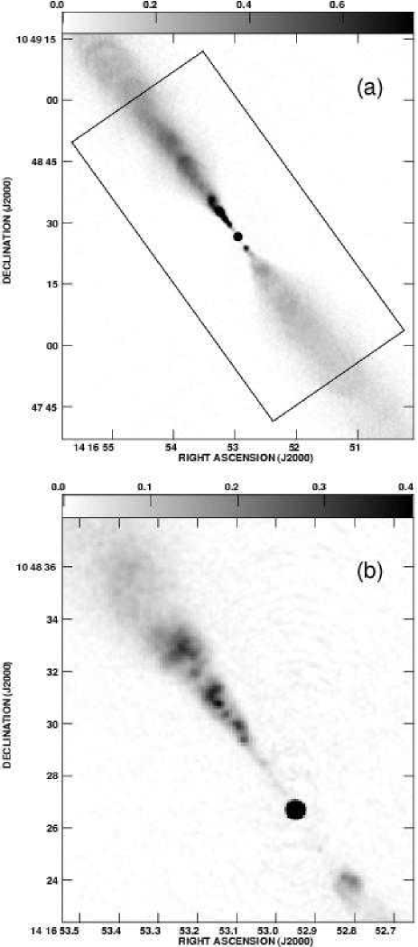
Figure 3: Grey-scales of total intensity for the jets of 3C 296 at 8.5 GHz, both from maximum-entropy images, corrected for attenuation by the primary beam. (a) Image at 0.75-arcsec resolution. The grey-scale range is 0 – 0.75 mJy beam^-1 and the box shows the modelled area (Sections 4 – 6). (b) Image at 0.25-arcsec resolution with a grey-scale range of 0 – 0.4 mJy beam^-1.

The overall structure of the source at 5.5-arcsec FWHM is shown in Fig. 1(a). This image emphasises that the lobes are well-defined, with sharp leading edges. With the possible exception of the innermost $\pm$15 arcsec, where the extended emission is very faint, the jets appear superimposed on the lobes everywhere. It is possible that the jets propagate (almost) entirely within the lobes, although the superposition may also be a projection effect. Fig. 1(b), which shows the same area at a resolution of 1.5 arcsec FWHM, emphasises that the boundaries between the jets and lobes are not precisely defined at 1.4 GHz, although the edges of the jets are marked by sharp brightness gradients.

In contrast, the lobe emission is almost invisible in an 8.5-GHz image at the same resolution (Fig. 2a). The transfer function of this grey-scale has been chosen to emphasise sub-structure (“arcs”) in the brightness distributions. These features are emphasised further and labelled in Fig. 2(b), which shows a Sobel-filtered version of the same image. The Sobel operator (Pratt, 1991) computes an approximation to $\mid\nabla(I)\mid$ and therefore highlights large brightness gradients. Arcs are observed in both jets, but appear to have two characteristic shapes: (i) concave towards the nucleus and approximately semicircular and (ii) oblique to the jet direction on either side of the jet but without large brightness gradients on-axis. They do not occupy the full width of the jets. All of the arcs in the main jet are of type (i); of those in the counter-jet, the inner three marked in Fig. 2(b) are of type (ii) but the outer two are of type (i). In Section 6.7, we interpret the structural differences in the main and counter-jet arcs as an effect of relativistic aberration.

Fig. 3 shows the inner jets of 3C 296 in grey-scale representations again chosen to emphasise the fine-scale structure. The initial “flaring”, i.e., decollimation followed by recollimation (Bridle, 1982), is clearest at 0.75-arcsec resolution (Fig. 3a), as is the ridge of emission along the axis of the main jet noted by Hardcastle et al. (1997); the innermost arcs are also visible. Our highest-resolution image (0.25 arcsec FWHM; Fig. 3b) shows the faint base of the main jet. This brightens abruptly at a distance of 2.7 arcsec from the nucleus; further out there is complex, non-axisymmetric knotty structure within a well-defined outer envelope. All of these features are typical of FR I jet bases (e.g. LB, CL, CLBC). There is only a hint of a knot in the counter-jet at 1.8 arcsec from the nucleus, opposite the faint part of the main jet, but integrating over corresponding regions between 0.5 and 2.7 arcsec in the main and counter-jets gives $I_{\rm j}/I_{\rm cj}\approx 2.7$. The counter-jet brightens at essentially the same distance from the nucleus as the main jet, but its prominent, non-axisymmetric, edge-brightened knot is significantly wider than the corresponding emission on the main jet side.

3.2 Spectrum

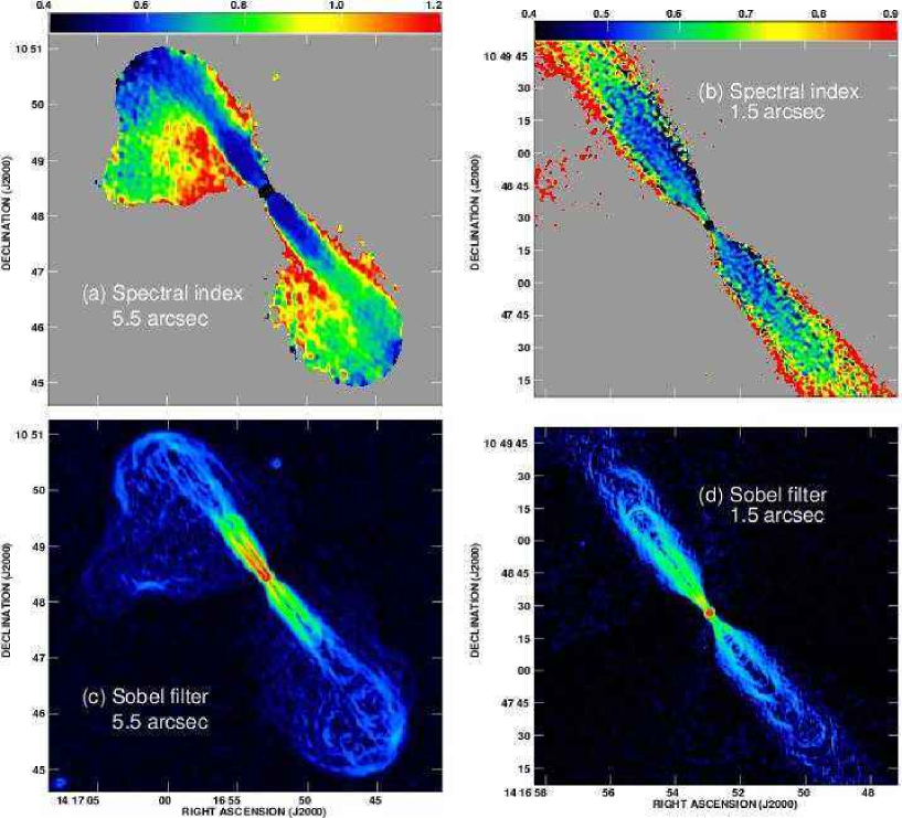
Figure 4: False-colour plots of spectral index and intensity gradients. (a) Spectral index between 1.48 and 8.5 GHz at a resolution of 5.5 arcsec FWHM. The spectral-index range is 0.4–1.2. (b) Spectral index between 1.4 and 8.5 GHz at a resolution of 1.5 arcsec FWHM. The spectral-index range is 0.4 – 0.9.In panels (a) and (b), values are plotted only if the rms error is $<$0.2; blanked pixels are coloured grey. (c) Sobel-filtered L-band image at 5.5 arcsec FWHM; (d) Sobel-filtered 8.5-GHz image at 1.5 arcsec FWHM.

The D-configuration observations at 8.5 GHz nominally sample a largest spatial scale of only 180 arcsec. Although the total angular extent of 3C 296 is 440 arcsec, the accurate calibration of our dataset and the fact that we have recovered the total flux of the source imply that we have enough information to construct a low-resolution image of spectral index, $\alpha$, between 8.5 and 1.48 GHz. This is shown in Fig. 4(a). We have also made a spectral-index image at 1.5 arcsec resolution between 8.5 and 1.41 GHz; here the values in the diffuse emission are not reliable, and we show only the inner jets (Fig. 4b). Sobel-filtered $I$ images at the two resolutions are shown for comparison in Figs 4(c) and (d).

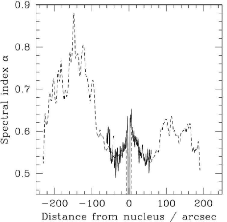
Figure 5: Profiles of the spectral index along the jets of 3C 296 in PA $-35.^{\circ}86$. Dashed line: $\alpha$ measured between 1.48 and 8.5 GHz at a resolution of 5.5 arcsec FWHM, along the jet ridge line from Fig. 4(a). Full line: $\alpha$ between 1.41 and 8.5 GHz at a resolution of 1.5 arcsec, averaged over $\pm$1.5″on either side of the jet axis, from Fig. 4(b).

Fig. 4(a) shows that the low-brightness regions of the lobes have significantly steeper spectra than the jets. Spectral indices in the jets at 5.5-arcsec resolution range from $\alpha=0.53$ close to the nucleus in both jets to $\alpha\approx 0.6$ in the main jet and $\alpha\approx 0.8$ in the counter-jet. The steepest-spectrum diffuse emission visible in Fig. 4(a) has $\alpha\approx 1.3$. As in other FR I objects (Katz-Stone & Rudnick, 1997; Katz-Stone et al., 1999), the jets appear to be superposed on steeper spectrum lobe emission, so there must be blending of spectral components. A steeper-spectrum component is present on both sides of the main and counter-jets, although it is more prominent to the SE. It is clearly visible and resolved from $\approx$17 arcsec outwards along the main jet. The apparent narrowness of the steep-spectrum rim within $\approx$50 arcsec of the nucleus in the counter-jet, is misleading, however. Much of the lobe emission detected at 1.5 GHz in this region (Fig. 1a) is too faint at 8.5 GHz to determine a reliable spectral index and the image in Fig. 4(a) is therefore blanked. Conversely, any superposed diffuse emission will have a small effect on the spectral index where the jet is bright. Only within roughly a beamwidth of the observed edge of the jet are the two contributions comparable, with a total brightness high enough for $\alpha$ to be determined accurately. The spectrum therefore appears steeper there (Fig. 4a). With higher sensitivity, more extended steep-spectrum emission should be detectable around the inner counter-jet.

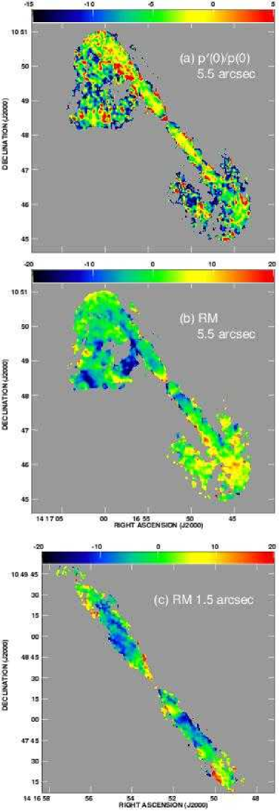
Figure 6: (a) Normalized polarization gradient $p^{\prime}(0)/p(0)$ from a fit to $p$ at frequencies of 8.5, 1.45 and 1.50 GHz over the range $-20$ to $+5$ m^-2. The resolution is 5.5 arcsec FWHM. (b) RM image at 5.5-arcsec FWHM resolution, from a fit to position angles at the frequencies used in panel (a). (c) RM at 1.5 arcsec from a fit to position angles at 8.5, 1.46 and 1.39 GHz. The labelled wedges for panels (b) and (c) are in units of rad m^-2. The areas covered by the panels correspond to Figs 1 for (a) and (b) and Fig. 2 for (c). Blanked pixels are coloured grey.

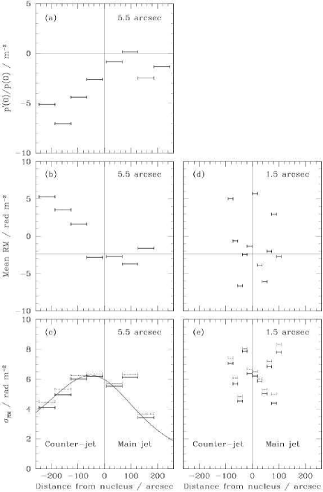
Figure 7: Profiles of RM and depolarization along the jet axis, taken to be in PA $-35^{\circ}.86$. Positive and negative distances refer to the main and counter-jet sides, respectively. Panels (a) – (c) show averages for boxes of length 60 arcsec (along the jet axis) and width 39 arcsec at a resolution of 5.5 arcsec FWHM. A $\pm$7.5-arcsec region around the core is excluded. (a) Mean normalized polarization gradient $\langle p^{\prime}(0)/p(0)\rangle$. (b) Mean RM. The horizontal line shows the estimated Galactic RM. (c) Rms RM. The full lines show $\sigma_{\rm RM}$ after a first-order correction for fitting error, the dotted lines show the uncorrected values $\sigma_{\rm RMraw}$ and the curve shows a simple model fitted by eye to the data (see text). (d) and (e) As (b) and (c), but at a resolution of 1.5 arcsec FWHM. The boxes are 18 arcsec long and are extended transverse to the jet to include all of the unblanked emission in Fig. 6(c). The excluded region around the core is $\pm 1.5$ arcsec.

Flatter-spectrum emission can be traced beyond the sharp outer bends in both jets, suggesting that the flow in the outer part of the radio structure remains coherent even after it deflects through a large angle, at least in projection. A comparison between the spectral-index image and a Sobel-filtered L-band image (Figs 4a and c) shows that the flatter-spectrum regions are bounded by high brightness gradients; they can therefore be separated both morphologically and spectrally from the surrounding steep-spectrum emission. In the NE lobe, the flatter-spectrum “extension” of the jet can be traced until it terminates at a region with an enhanced intensity (and intensity gradient) on the South edge of the lobe (Figs 1a, 4a and c).

The spectral structure therefore suggests that the jets deflect when they reach the ends of the lobes rather than disrupting completely. In FR I sources such as 3C 296, no strong shocks (hot-spots) are formed, implying that the generalised internal Mach number of the flow, ${\cal M}=\Gamma\beta/\Gamma_{\rm s}\beta_{\rm s}\la 1$, where $\beta_{\rm s}c$ is the internal sound speed and $\Gamma_{\rm s}=(1-\beta_{\rm s}^{2})^{-1/2}$ (Königl, 1980). For an ultrarelativistic plasma, $\beta_{\rm s}=3^{-1/2}$, so strong shocks need not occur at the bends even if the flow remains mildly relativistic (e.g. we infer a transonic flow decelerating from $\beta\approx 0.8$ to $\beta\approx 0.2$ in 3C 31; Laing & Bridle 2002b). In 3C 296, our models imply that $\beta\approx 0.4$ on-axis at a projected distance of 40 arcsec from the nucleus, with a possible deceleration to $\beta\la 0.1$ at larger distances (Section 6.3).

It is plausible that the spectra in the lobe regions of 3C 296 have been steepened by a combination of synchrotron, inverse Compton and adiabatic losses but it is not clear from the spectral-index image whether the jets and their extensions propagate within the steep-spectrum lobes (as in the standard model for FR II sources) or appear superimposed on them.

At higher resolution (Fig. 4b), there are variations in $\alpha$ both along and transverse to the jets. Fig. 5 shows a longitudinal profile of spectral index along the axis within 60 arcsec of the nucleus, where the superposed diffuse, steep-spectrum emission has a negligible effect. There is good agreement between the spectral indices measured at 1.5 and 5.5-arcsec resolution in this area. The spectral index close to the nucleus in both jets is $\approx$0.62. The spectrum then flattens with distance from the nucleus to $\alpha\approx 0.53$ at 40 arcsec. Further from the nucleus, the spectrum steepens again (Fig. 4b), but lobe contamination becomes increasingly important and it is not clear that we are measuring the true spectrum of the jet. The flattening with increasing distance in the first 40 arcsec of both jets is in the opposite sense to that expected from contamination by lobe emission, however. The few other FR I jets observed with adequate resolution and sensitivity (none of which are superposed on lobes) show a similar spectral flattening with distance: PKS 1333$-$33 (Killeen et al., 1986), 3C 449 (Katz-Stone & Rudnick, 1997), NGC 315 (Laing et al., 2006), and NGC 326 (Murgia, private communication).

A comparison of Figs 4(b) and (d) shows that the spectral index is flatter in both jets roughly where the more distinct arcs are seen, but the arcs are not recognisable individually on the spectral index images. They contain only a few tens of percent of the total jet emission along their lines of sight, so a small difference in spectral index between them and their surroundings would not be detectable. The apparent narrowness of the steeper-spectrum ($\alpha\approx 0.9$) rim observed at the edges of the jets in Fig. 4(b) results from the superposition of jet and lobe emission, just as at lower resolution. This effect confuses any analysis of intrinsic transverse spectral gradients in the jets, such as those in the flaring region of NGC 315 (Laing et al., 2006), but there are hints that the intrinsic spectrum flattens slightly away from the axis within $\approx$30 arcsec of the nucleus in 3C 296 (Fig. 4b).

At 0.4-arcsec resolution, we measure $\alpha\approx 0.67$ between 4.9 and 8.5 GHz for the bright region of the main jet between 2 and 8 arcsec from the nucleus and $\alpha\approx 0.57$ for the bright knot at the base of the counter-jet.

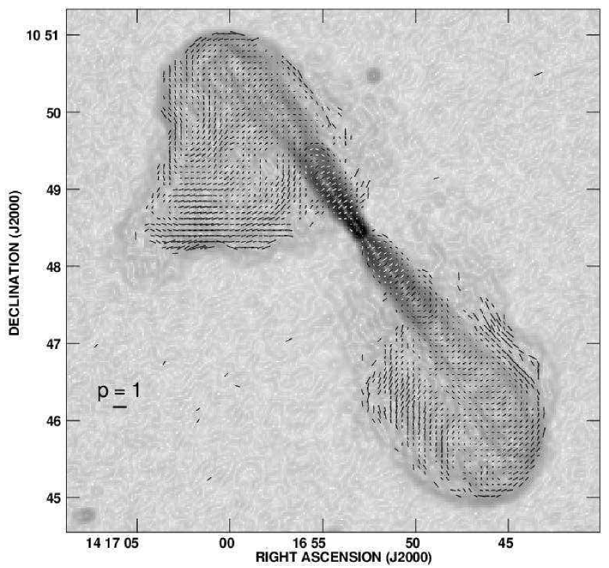
Figure 8: Vectors with lengths proportional to the degree of polarization at 8.5 GHz and directions along the apparent magnetic field, superimposed on a grey-scale of the total intensity gradient (Sobel-filtered image) at 1.5 GHz. The resolution is 5.5 arcsec FWHM. The vector directions are derived from the 3-frequency RM fits where there is adequate signal-to-noise ratio; elsewhere, the 8.5-GHz position angles are corrected using the mean RM over the area of the image. Vectors are plotted where $P\geq 2\sigma_{P}$ and $I\geq 5\sigma_{I}$.

3.3 Faraday rotation and depolarization

Comparison of lower-resolution images at 1.7 and 0.6 GHz showed that the SW (counter-jet) lobe depolarizes more rapidly than the NE (main jet) lobe (Garrington et al., 1996). We derived the polarization gradient $p^{\prime}(0)=dp/d(\lambda^{2})$ and the polarization at zero wavelength, $p(0)$ from a linear fit to the degree of polarization as a function of $\lambda^{2}$, $p(\lambda^{2})\approx p(0)+p^{\prime}(0)\lambda^{2}$, using 5.5-arcsec resolution images at 8.5, 1.50 and 1.45 GHz. The linear approximation is adequate for the low depolarization seen in 3C 296 and allows us to use images at more than two frequencies to reduce random errors. We show an image of $p^{\prime}(0)/p(0)$ (closely related to depolarization) in Fig. 6(a). There is a gradient along the jets, in the sense that the outer counter-jet is more depolarized than the main jet; we show a profile along the axis in Fig. 7(a). Both lobes show significant depolarization: $\langle p^{\prime}(0)/p(0)\rangle=-3.7$ m^-2 and $-5.8$ m^-2 for the NE and SW lobes, respectively, corresponding to depolarizations of 0.84 and 0.75 at 1.45 GHz. As can be seen from Figs 6(a) and 7(a), the diffuse emission in the NE lobe is significantly more depolarized ($\langle p^{\prime}(0)/p(0)\rangle=-4.8$ m^-2) than the main jet. In the SW lobe, the depolarization of the diffuse emission ($\langle p^{\prime}(0)/p(0)\rangle=-6.2$ m^-2) is comparable to that of the counter-jet measured further than 100 arcsec from the nucleus (Fig. 7a).

The integrated Faraday rotation measure (RM) for 3C 296 is $-3\pm 2$ rad m^-2 (Simard-Normandin, Kronberg & Button, 1981) and a mean value of 0 rad m^-2 with an rms dispersion of 4 rad m^-2 was derived by Leahy, Pooley & Riley (1986) from three-frequency imaging at a resolution of $6\times 22$ arcsec² FWHM. We imaged the distribution of RM at 5.5 arcsec resolution, fitting to ${\bf E}$-vector position angles, $\chi$, at 8.5, 1.50 and 1.45 GHz. Given the closeness of the two lower frequencies, we have poor constraints on the linearity of the $\chi$ – $\lambda^{2}$ relation, but the values of RM are sufficiently small that we can be sure that there are no $n\pi$ ambiguities (this is confirmed by comparison with the 2.7-GHz images of Birkinshaw, Laing & Peacock 1981). The resulting RM image is shown in Fig. 6(b). The mean RM is $-0.4$ rad m^-2, with an rms of 6.1 rad m^-2 and a total spread of $\pm$20 rad m^-2. Profiles of mean and rms RM along the jet axis are shown in Figs 7(b) and (c). We made a first-order correction to the rms RM, $\sigma_{\rm RMraw}$, by subtracting the fitting error $\sigma_{\rm fit}$ in quadrature to give $\sigma_{\rm RM}=(\sigma_{\rm RMraw}^{2}-\sigma_{\rm fit}^{2})^{1/2}$. Both raw and corrected values are plotted in Fig. 7(c). There is a clear large-scale gradient in RM across the counter-jet lobe, roughly aligned with the axis and with an amplitude of $\approx$8 rad m^-2. Fluctuations on a range of smaller scales are also evident. The rms RM peaks close to the nucleus and decreases by a factor of 1.5 – 2 by 200 arcsec away from it (Fig. 7c).

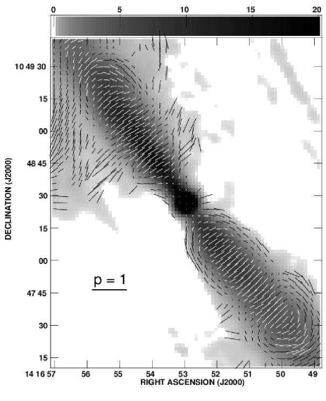
Figure 9: Vectors with lengths proportional to the degree of polarization at 8.5 GHz and directions along the apparent magnetic field, superimposed on a grey-scale of total intensity at the same frequency. A square root transfer function has been used to emphasise the diffuse emission around the main jet. The resolution is 5.5 arcsec FWHM. The vector directions are derived from 3-frequency RM fits where there is adequate signal-to-noise ratio; elsewhere, the 8.5-GHz position angles are corrected using the mean RM over the area of the image. Vectors are plotted where $P\geq 2\sigma_{P}$ and $I\geq 5\sigma_{I}$.

At 1.5-arcsec resolution, we made 3-frequency RM fits to images at 1.39, 1.46 and 8.5 GHz (Fig. 6c). Note that the largest scale sampled completely in this image is $\approx$40 arcsec. Profiles of mean and rms RM at this resolution are shown in Figs 7(d) and (e). There are no systematic trends in either quantity within 100 arcsec of the nucleus.

Our data are qualitatively consistent with the results of Garrington et al. (1996) in the sense that we see somewhat more depolarization in the counter-jet lobe at 5.5-arcsec resolution. The corresponding profile of RM fluctuations is quite symmetrical, however. If we calculate the depolarization expected with the beam used by Garrington et al. (1996) between 1.7 and 0.6 GHz using the observed degree of polarization at 1.4 GHz and the RM image at 5.5-arcsec resolution, we find no gross differences between the lobes. This analysis neglects spectral variations across the source and depolarization due to any mechanism other than foreground Faraday rotation on scales $\ga$5.5 arcsec, however.

A simple model in which the variations in RM result from foreground field fluctuations in a spherically-symmetric hot gas halo is reasonable for 3C 296: the model profile plotted in Fig. 7(c) was derived following the prescription in Laing et al. (2006), assuming an angle to the line of sight of $58^{\circ}$ (Section 6.2) and fitted by eye to the data. For the derived core radius $r_{c}=300$ arcsec, the asymmetries in the predicted $\sigma_{\rm RM}$ profile for angles to the line of sight $\ga 50^{\circ}$ are small and reasonably consistent with our observations. A full analysis must, however, include the gradient of RM across the counter-jet lobe and the enhanced depolarization seen in that region, neither of which follow the same profile as the rms RM. The large-scale gradient is extremely unlikely to be Galactic, as the total Galactic RM estimated from the models of Dineen & Coles (2005) is only $-2.4$ rad m^-2 and fluctuations on 200-arcsec scales are likely to be even smaller. The gradient must, therefore, be local to 3C 296 (a similar large-scale RM gradient, albeit of much larger amplitude, was observed in Hydra A by Taylor & Perley 1993). We defer a quantitative analysis of the Faraday rotation and depolarization until XMM-Newton imaging of the hot gas on the scale of the lobes is available for 3C 296.

3.4 Apparent magnetic field

We show the direction of the apparent magnetic field, rotated from the zero-wavelength E-vector position angles by 90^∘. Over much of the observed region, this can be derived directly from the $\chi$ – $\lambda^{2}$ fit. The 8.5-GHz images generally have more points with significant polarization than those at lower frequencies, however. At points with significant polarized signal at 8.5 GHz but no RM measurement, we determined the apparent magnetic-field direction using the observed 8.5-GHz position angle and the mean RM for the region. The maximum error introduced by this procedure is $\approx 1.4^{\circ}$ provided that the RM distribution is no wider than in Fig. 6(b). The apparent field directions are shown for the whole source at 5.5 arcsec FWHM resolution in Fig. 8, in more detail for a small region around the nucleus at the same resolution in Fig. 9, and for the jets at 1.5-arcsec FWHM resolution in Fig. 10. The vector lengths in these plots are proportional to the degree of polarization at 8.5 GHz, corrected to first order for Ricean bias (Wardle & Kronberg, 1974); this is equal to $p(0)$ within the errors at all points where we have sufficient signal-to-noise to estimate depolarization (Section 3.3).

As noted by Leahy & Perley (1991), the apparent magnetic field in the lobe emission is circumferential, with a high degree of polarization at the edges of the lobes. The magnetic field directions are well aligned with the ridges of the steepest intensity gradients, as shown by the superposition on the Sobel-filtered L-band image (Fig. 8). The jets show mainly transverse apparent field at 5.5 arcsec resolution, but the low-brightness regions around them do not all exhibit the same pattern of polarization. Those to the NW of both jets show $p\ga 0.4$ with the field ordered parallel to the jet axis. Those to the SE of the main jet are comparably polarized but with the magnetic field oblique to the jet axis while those to the SE of the counter-jet are only weakly polarized. Both lobes contain polarized structure related to the spectral-index structure evident in Fig. 4(a). The field structure in the S lobe is suggestive of a flow that turns through 180^∘ but retains a transverse-field configuration after the bend. That in the N lobe is suggestive of a jet extension whose magnetic configuration changes from parallel immediately after the bend to transverse. The emission at the S edge of the lobe where there is a locally strong intensity gradient also exhibits a high ($p\ga 0.6$) linear polarization with the magnetic field tangential to the lobe boundary, i.e. transverse to the jet “extension” suggested by our spectral data.

At 1.5-arcsec resolution, the jet field structure is revealed in more detail (Fig. 10). Longitudinal apparent field is visible at the edges of both jets, most clearly close to the nucleus and at $\approx$60 arcsec from it. There are enhancements in polarization associated with the two outermost arcs in each jet: in all four cases the apparent field direction is perpendicular to the maximum brightness gradient.

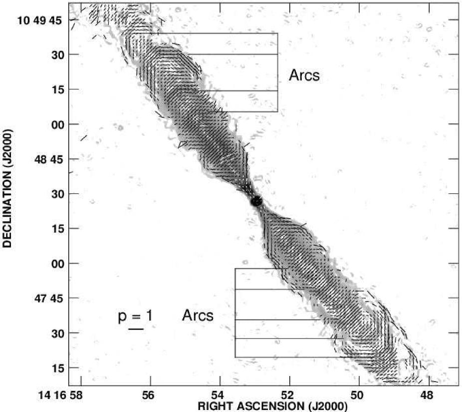
Figure 10: Vectors with lengths proportional to the degree of polarization at 8.5 GHz and directions along the apparent magnetic field, superimposed on a grey-scale of Sobel-filtered total intensity at the same frequency. The resolution is 1.5 arcsec FWHM. The vector directions are derived from 3-frequency RM fits where there is adequate signal-to-noise ratio; elsewhere, the 8.5-GHz position angles are corrected using the mean RM of the image. Vectors are plotted where $P\geq 3\sigma_{P}$ and $I\geq 5\sigma_{I}$. The “arcs” are those marked in Fig. 2(b).

The 8.5-GHz $Q$ and $U$ images at 0.75 and 0.25 arcsec FWHM used for modelling have been corrected for Faraday rotation using the 1.5-arcsec RM images interpolated onto a finer grid. The corresponding apparent field directions are discussed in Section 5.2.

4 The model

4.1 Assumptions

Our principal assumptions are as as in LB, CL and CLBC:

1. FR I jets may be modelled as intrinsically symmetrical, antiparallel, axisymmetric, stationary laminar flows. Real flows are, of course, much more complex, but our technique will still work provided that the two jets are statistically identical over our averaging volumes.

2. The jets contain relativistic particles with an energy spectrum $n(E)dE=n_{0}E^{-(2\alpha+1)}dE$ and an isotropic pitch-angle distribution, emitting optically-thin synchrotron radiation with a frequency spectral index $\alpha$. We adopt a spectral index of $\alpha=0.60$ derived from an average of the spectral-index image in Fig. 4(b) over the modelled region. The maximum degree of polarization is then $p_{0}=(3\alpha+3)/(3\alpha+5)=0.705$.

3. The magnetic field is tangled on small scales, but anisotropic (Laing, 1981; Begelman et al., 1984; Laing & Bridle, 2002a; Laing, Canvin & Bridle, 2006).

4.2 Outline of the method

It is well known that synchrotron radiation from intrinsically symmetrical, oppositely directed bulk-relativistic outflows will appear one-sided as a result of Doppler beaming. The jet/counter-jet ratio, $I_{\rm j}/I_{\rm cj}=[(1+\beta\cos\theta)/(1-\beta\cos\theta)]^{2+\alpha}$ for a constant-speed, one-dimensional flow with isotropic emission in the rest frame. The key to our approach is that aberration also acts differently on linearly-polarized radiation from the approaching and receding jets, so their observed polarization images represent two-dimensional projections of the magnetic-field structure viewed from different directions $\theta_{\rm j}^{\prime}$ and $\theta_{\rm cj}^{\prime}$ in the rest frame of the flow: $\sin\theta_{\rm j}^{\prime}=\sin\theta[\Gamma(1-\beta\cos\theta)]^{-1}$ and $\sin\theta_{\rm cj}^{\prime}=\sin\theta[\Gamma(1+\beta\cos\theta)]^{-1}$. This is the key to breaking the degeneracy between $\beta$ and $\theta$ and to estimating the physical parameters of the jets (Canvin & Laing, 2004).

We have developed a parameterized description of the jet geometry, velocity field, emissivity and magnetic-field ordering. We calculate the emission from a model jet in $I$, $Q$ and $U$ by numerical integration, taking full account of relativistic aberration and anisotropic rest-frame emission, convolve to the appropriate resolution and compare with the observed VLA images. We optimize the model parameters using the downhill simplex method with $\chi^{2}$ (summed over $I$, $Q$ and $U$) as a measure of goodness of fit (note that the modelling is not affected by Ricean bias as we fit to Stokes $I$, $Q$ and $U$ directly). The method is described fully by LB, CL and CLBC.

Our method is restricted to the vicinity of the nucleus, where we expect that relativistic effects dominate over intrinsic or environmental asymmetries. The modelled region for 3C 296 (indicated by the box on Fig. 3a) is limited in extent by slight bends in the jets at $\approx$45 arcsec from the nucleus. Contamination by surrounding lobe emission also becomes significant at larger distances.

4.3 Functional forms for geometry, velocity, magnetic field and emissivity

The functional forms used for velocity, emissivity and field ordering are identical to those described by CLBC except for a very small change to the emissivity profile (Section 4.3.4). We briefly summarize the concepts in this Section and give the functions in full for reference in the Appendix (Table 4).

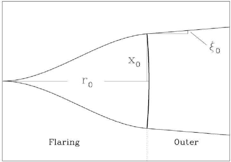
Figure 11: The geometry of the jet, showing the flaring and outer regions and the quantities which define the shape of its outer surface.

4.3.1 Geometry

The assumed form for the jet geometry (Fig. 11) is that used by CL and CLBC. The jet is divided into a flaring region where it first expands and then recollimates, and a conical (almost cylindrical) outer region. The geometry is defined by the angle to the line of sight, $\theta$, the distance from the nucleus of the transition between flaring and outer regions, $r_{0}$, the half-opening angle of the outer region, $\xi_{0}$ and the width of the jet at the transition, $x_{0}$ (all fitted parameters).

We assume laminar flow along streamlines defined by an index $s$ ($0\leq s\leq 1$) where $s=0$ corresponds to the jet axis and $s=1$ to its edge. In the outer region, the streamlines are straight and in the flaring region the distance of a streamline from the axis of the jet is modelled as a cubic polynomial in distance from the nucleus. Distance along a streamline is measured by the coordinate $\rho$, which is exactly equal to distance from the nucleus for the on-axis streamline. The streamline coordinate system is defined in Appendix A.

4.3.2 Velocity

The form of the velocity field is as used by CL and CLBC. The on-axis profile is divided into three parts: roughly constant, with a high velocity $\beta_{1}$ close to the nucleus; a linear decrease and a roughly constant but lower velocity $\beta_{0}$ at large distances. The profile is defined by four free parameters: the distances of the two boundaries separating the regions and the characteristic inner and outer velocities. Off-axis, the velocity is calculated using the same expressions but with truncated Gaussian transverse profiles falling to fractional velocities varying between $v_{1}$ and $v_{0}$ (Table 4).

4.3.3 Magnetic field

We define the rms components of the magnetic field to be $\langle B_{l}^{2}\rangle^{1/2}$ (longitudinal, parallel to a streamline) and $\langle B_{t}^{2}\rangle^{1/2}$ (toroidal, orthogonal to the streamline in an azimuthal direction). We initially included a radial field component in the model, exactly as for NGC 315 (CLBC). The best-fitting solution had a small radial component on the jet axis, but not elsewhere, and the fitted coefficients were everywhere consistent with zero. The improvement in $\chi^{2}$ resulting from inclusion of a radial component was also very small (see Section 4.4). We therefore present only models in which the radial field component is zero everywhere. The longitudinal/toroidal field ratio varies linearly with streamline index as in CLBC (Table 4) .

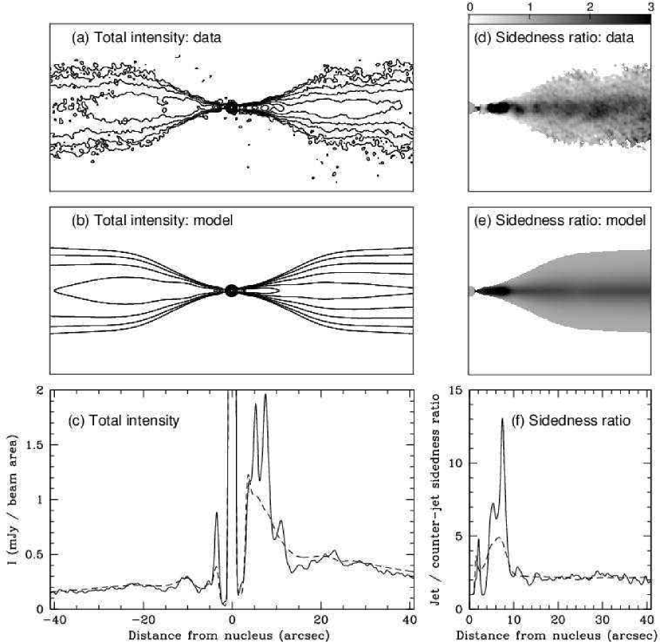
Figure 12: Comparison between data and model at a resolution of 0.75 arcsec. The displayed region is $\pm$40.95 arcsec from the nucleus along the jet axis and the scale is indicated at the bottom of the Figure. (a) Observed contours. The levels are $-1$, 1, 2, 4, 8, 16, 32, 64, 128, 256, 512, 1024, 2048, 4096 $\times$ 20 $\mu$Jy beam^-1. (b) Model contours, with the same levels as in panel (a). (c) Profiles of total intensity along the jet axis. Full line: data; dashed line: model. (d) Grey-scale of observed jet/counter-jet sidedness ratio, in the range 0 – 3, chosen to show the variations in the outer parts of the modelled region. (d) Grey-scale of model sidedness ratio. (e) Profiles of sidedness ratio along the jet axis. Full line: data; dashed line: model.

4.3.4 Emissivity

We take the proper emissivity to be $\epsilon h$, where $\epsilon$ is the emissivity in $I$ for a magnetic field $B=\langle B_{l}^{2}+B_{t}^{2}\rangle^{1/2}$ perpendicular to the line of sight and $h$ depends on field geometry: for $I$, $0\leq h\leq 1$ and for $Q$ and $U$ $-p_{0}\leq h\leq+p_{0}$. We refer to $\epsilon$, loosely, as ‘the emissivity’. For a given spectral index, it is a function only of the rms total magnetic field and the normalizing constant of the particle energy distribution, $\epsilon\propto n_{0}B^{1+\alpha}$.

As in CL and CLBC, the majority of the longitudinal emissivity profile is modelled by three power laws $\epsilon\propto\rho^{-E}$, with indices $E=E_{\rm in}$, $E_{\rm mid}$ and $E_{\rm out}$ (in order of increasing distance from the nucleus). The inner emissivity region corresponds to the faint inner jets before what we will call the brightening point. The middle region describes the bright jet base and the outer region the remainder of the modelled area. We have adopted slightly different ad hoc functional forms for the short connecting sections between these regions in CL, CLBC and the present paper. For 3C 296, we allow a discontinuous increase in emissivity at the end of the innermost region, followed by a short section with power-law index $E_{\rm knot}$, introduced to fit the first knots in the main and counter-jets. We adopt truncated Gaussian profiles for the variation of emissivity with streamline index. The full functional forms for the emissivity (with the names of some variables changed from CLBC in the interest of clarity) are again given in Table 4.

4.4 Fitting, model parameters and errors

The noise level for the calculation of $\chi^{2}$ for $I$ is estimated as $1/\sqrt{2}$ times the rms of the difference between the image and a copy of itself reflected across the jet axis. For linear polarization, the same level is used for both $Q$ and $U$. This is the mean of $1/\sqrt{2}$ times the rms of the difference image for $Q$ and the summed image for $U$, since the latter is antisymmetric under reflection for an axisymmetric model. This prescription is identical to that used by LB, CL and CLBC. The region immediately around the core is excluded from the fit.

We fit to the 0.25-arcsec FWHM images within 8.75 arcsec of the nucleus and to the 0.75-arcsec FWHM images further out. In doing so, we implicitly assume that the jet structure visible at 8.5 GHz is not significantly contaminated by superposed lobe emission. For total intensity, this is justified by the faintness of the lobe emission close to the jet even at much lower resolution (Fig. 9); we discuss the possibility of contamination of the polarized jet emission in Section 5.3. In our initial optimizations, the quantities defining the shape of the jet projected on the plane of the sky were allowed to vary. These were then fixed and the remaining parameters were optimized, using only data from within the outer isophote of the model.

We derive rough uncertainties, as in LB, CL and CLBC, by varying individual parameters until the increase in $\chi^{2}$ corresponds to the formal 99% confidence level for independent Gaussian errors. These estimates are crude (they neglect coupling between parameters), but in practice give a good representation of the range of qualitatively reasonable models. The number of independent points (2588 in each of 3 Stokes parameters) is sufficiently large that we are confident in the main features of the model. The reduced $\chi^{2}_{\rm red}=0.72$, suggesting that our noise model is oversimplified. A model with a radial field component and a more general variation of field-component ratios with streamline index has $\chi^{2}_{\rm red}=0.69$, but the coefficients describing the radial field are all consistent with zero; in any case, the remaining model parameters are all identical to within the quoted errors with those given here.

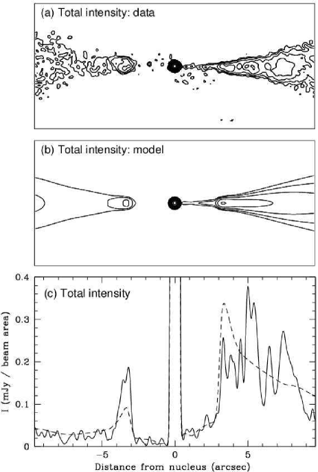
Figure 13: Comparison between data and model at a resolution of 0.25 arcsec. The displayed region is $\pm$9.625 arcsec from the nucleus along the jet axis and the scale is indicated at the bottom of the Figure. (a) Observed contours. The levels are $-1$, 1, 2, 4, 8, 16, 32, 64, 128, 256, 512, 1024, 2048, 4096 $\times$ 20 $\mu$Jy beam^-1. (b) Model contours, with the same levels as in panel (a). (c) Profiles of total intensity along the jet axis. Full line: data; dashed line: model.

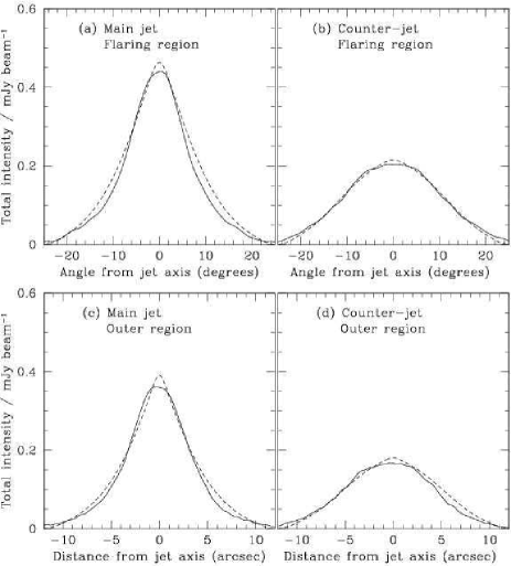
Figure 14: Comparison between averaged transverse profiles of total intensity in the main and counter-jets at a resolution of 0.75 arcsec. (a) main jet, (b) counter-jet in the flaring region. The profiles are generated by averaging along along radii between 15 and 27 arcsec from the nucleus and plotting against angle from the jet axis. (c) main jet, (d) counter-jet in the outer region. The profiles are generated by averaging along the jet between 27 and 40.95 arcsec from the nucleus and plotting against distance from the jet axis. In all panels, the data are represented by full lines and the model by dashed lines.

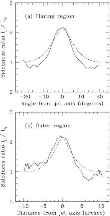
Figure 15: Comparison between averaged transverse profiles of jet/counter-jet sidedness ratio for data and model at a resolution of 0.75 arcsec. Full line: data; dashed line: model. (a) Averages along radii from the nucleus in the flaring region between 15 and 27 arcsec. (b) Average along the jet axis in the outer region between 27 and 40.95 arcsec.

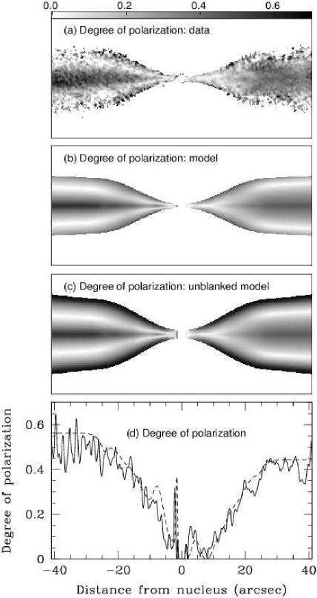
Figure 16: Comparison between the degree of polarization, $p=P/I$, of the data and model at a resolution of 0.75 arcsec. The displayed region is $\pm$40.95 arcsec from the nucleus along the jet axis and the scale is indicated at the bottom of the Figure. (a) Grey-scale of observed degree of polarization, in the range 0 – 0.7. Points are only plotted if the total intensity $I>5\sigma_{I}$ (Table 2). (b) Grey-scale of the model degree of polarization in the same range, with the same blanking as in panel (a). (c) As in (b), but with no blanking applied. (d) Profiles of $p$ along the jet axis. Full line: data (all points have $I>5\sigma_{I}$, so no blanking has occurred); dashed line: model (also unblanked).

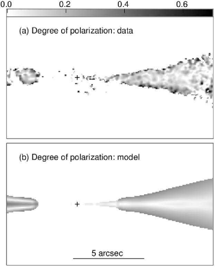
Figure 17: Comparison between the degree of polarization, $p=P/I$, of the data and model at a resolution of 0.25 arcsec. The displayed region is from $-5$ to $+9.625$ arcsec from the nucleus along the jet axis and the scale is indicated by the labelled bar. The cross shows the position of the core. (a) Grey-scale of observed degree of polarization, in the range 0 – 0.7. Points are only plotted if the total intensity $I>5\sigma_{I}$ (Table 2). (b) Grey-scale of the model degree of polarization with the same range and blanking as in panel (a).

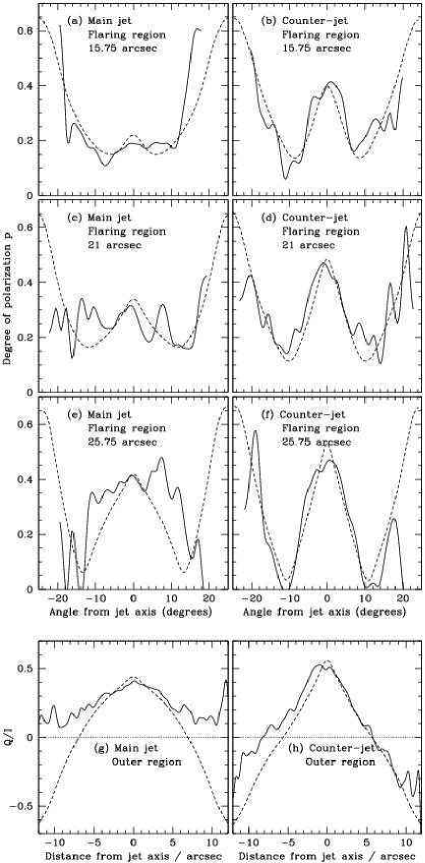
Figure 18: Transverse profiles of the degree of polarization for the main jet (left) and counter-jet (right) at representative distances from the nucleus. The resolution is 0.75 arcsec FWHM. In all panels, the data are represented by full lines and the model by dashed lines. (a) – (f): flaring region. The profiles are generated by taking scalar averages of $p$ along radii from the nucleus and plotting against angle from the jet axis. (a) and (b): 15 – 16.5 arcsec from the nucleus; (c) and (d): 20.25 – 21.75 arcsec; (e) and (f) 25 – 26.5 arcsec. Panels (g) – (h): averages of $Q/I$ along the jets between 27 and 40.95 arcsec from the nucleus, plotted against distance from the jet axis.

5 Comparison between models and data

5.1 Total intensity

The observed and modelled total intensities and jet/counter-jet sidedness ratios are compared in Figs 12 – 15. Figs 12 and 13 show images and longitudinal profiles at 0.75 and 0.25 arcsec resolution; averaged transverse profiles of total intensity and sidedness ratio are plotted in Figs 14 and 15.

The following total-intensity features are described well by the model:

1. The main jet is faint and narrow within $\approx$3  arcsec of the nucleus; such emission as can be seen from the counter-jet is consistent with a similar, but fainter brightness distribution (Fig. 13).

2. At 3 arcsec, there is a sudden increase in brightness on both sides of the nucleus.

3. The bright region at the base of the main jet extends to a distance of $\approx$13 arcsec from the nucleus; except for the initial bright knot, the counter-jet is much fainter relative to the main jet in this region (Fig 12f).

4. The jet/counter-jet sidedness ratio also shows a ridge of nearly constant amplitude from 10 arcsec to the end of the modelled region (Figs 12d – f). The ratio varies from 2.2 on-axis to $\approx 1$ at the edge of the jet in the outer part of the flaring region and in the outer region (Figs 15a, b).

5. The transverse total-intensity profiles from 15 arcsec to the end of the modelled region are accurately reproduced (Fig. 14).

5.2 Linear polarization

Grey-scales and longitudinal profiles of the degree of polarization for model and data at a resolution of 0.75 arcsec are compared in Fig. 16 and grey-scales of $p$ at 0.25-arcsec resolution are shown in Fig. 17. The model grey-scales in the former figure are plotted for $I>5\sigma_{I}$, to allow direct comparison with the observations, and without blanking, to show the polarization of the faint emission predicted at the edges of the jets. The observed polarization varies quite rapidly with distance from the nucleus in the flaring region, so a transverse profile of $p$ averaged over a large range of distances is not useful. We have, instead, plotted profiles at three representative positions, each averaged over 1.5 arcsec in distance from the nucleus (Figs 18a – f). Since the position angles vary significantly across the jet, we calculated scalar averages of $p$. In the outer region, the transverse $p$ profile is almost independent of distance, but the polarization at the edges of the jets in the outer region is difficult to see on the 0.75-arcsec resolution blanked images profiles, since individual points have low signal-to-noise ratios. In order to improve the accuracy of the transverse profiles we need to average over $Q$ and $U$ (as is done by the model fit) rather than the scalar $p$. To do this, we changed the origin of position angle to be along the jet axis. An apparent field parallel or orthogonal to the jet axis then appears entirely in the $Q$ Stokes parameter (and we verified that $U$ was indeed small). We then integrated $Q$ and $I$ along the jet axis and divided to give the profiles of $Q/I$ shown in Figs 18(g) and (h). The sign convention is chosen so $Q>0$ for a transverse apparent field and $Q<0$ for a longitudinal one. Finally, we plot vectors whose lengths are proportional to $p$ and whose directions are those of the apparent magnetic field in Figs 19 (0.75 arcsec) and 20 (0.25 arcsec) with two different blanking levels as in Fig. 16. All images of the observed degree of polarization have first-order corrections for Ricean bias (Wardle & Kronberg, 1974).

The following features of the polarized brightness distribution are well fitted by the model.

1. Both jets show the characteristic pattern of transverse apparent field on-axis with parallel field at the edges in the flaring region.

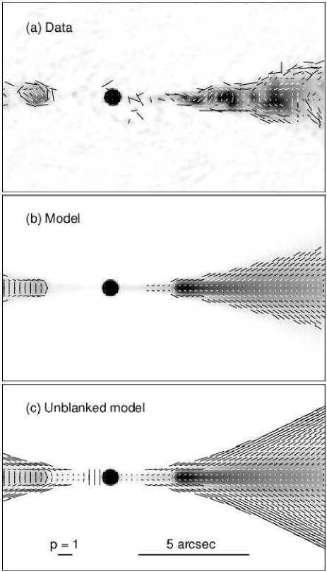
Figure 20: Vectors with lengths proportional to the degree of polarization, $p$, and directions along the apparent magnetic field, superimposed on grey-scales of total intensity. The resolution is 0.25 arcsec. The polarization and angular scales are indicated by the labelled bars in the lowest panel and the areas plotted are the same as those in Fig. 17. (a) data; (b) and (c) model. In panels (a) and (b), vectors are plotted only where $I>5\sigma_{I}$ (Table 2); no blanking has been applied in panel (c).

2. The parallel-field edge of the main jet is visible throughout the bright region at high resolution, albeit with low signal-to-noise ratio (Fig. 20). On-axis, the degree of polarization is significantly lower.

3. At high resolution, the apparent field at the base of the counter-jet appears to be “wrapped around” the bright knot (Fig. 20).

4. The longitudinal profile of $p$ (Fig. 16d) is matched well, reproducing the significant differences between the two jets.

5. The transition between longitudinal and transverse apparent field (where $p=0$) in the main jet is placed correctly at a distance of 8 arcsec from the nucleus (Figs 19, 16d).

6. In contrast, the counter-jet shows transverse apparent field on-axis even very close to the core (Figs 19a and c).

7. The asymptotic value of $p$ at distances from the nucleus $\ga$30 arcsec is larger in the counter-jet ($p\approx 0.5$) than in the main jet ($p\approx 0.4$).

8. The ridge of transverse apparent field is broader in the main jet than the counter-jet at distances from the nucleus $\ga$25 arcsec (Figs 16a – c, 18g – h, 19).

9. The evolution of the transverse polarization profiles with distance from the nucleus in the flaring region, which differ considerably between the two jets, are modelled accurately (Figs 18a – f, 19).

10. The apparent field at the edge of the outer region of the counter-jet is longitudinal, with a degree of polarization approaching the theoretical maximum of $p_{0}\approx 0.7$ (Fig. 18h).

5.3 Critique

Several features of the total-intensity distribution close to the nucleus are not well described by the model. The main problem is that the brightness distributions in both jets show erratic fluctuations causing the local jet/counter-jet sidedness ratio to increase with distance from the nucleus. Our models postulate a decelerating flow, so the jet/counter-jet ratio is expected to decrease monotonically with distance. In fact, the sidedness ratio has a low value at the position of the first knot in the counter-jet, 3 arcsec from the nucleus, compared with its typical value $\approx$10 between 4 and 9 arcsec: effectively, the first counter-jet knot is roughly a factor of two brighter than would be expected. The main jet base can be fit more accurately by a model with less low-velocity emission close to the brightening point, but the counter-jet knot is then eliminated completely and the overall $\chi^{2}$ is increased. The model for the main jet base also predicts slightly too narrow a brightness distribution (Fig. 13a and b): the fit to the longitudinal $I$ profile of the main jet at high resolution (Fig. 13c) is reasonable, but at lower resolution, where the jet is partially resolved, it appears worse (Fig. 12c). As in all of the other sources we have modelled, 3C 296 shows deviations from axisymmetry and erratic intensity variations in the bright region (Figs 3b and 13): we cannot fit these.

The counter-jet is slightly wider than the main jet in the flaring region: Fig. 21 shows a comparison of the 20 $\mu$Jy beam^-1 isophotes at 0.75 arcsec resolution. An inevitable consequence is that $I_{\rm j}/I_{\rm cj}<1$ at the edges of the jet. This is shown most clearly in the averaged transverse sidedness profiles of Fig. 15. In the flaring region, averaging between 15 and 27 arcsec from the nucleus, the minimum value of $I_{\rm j}/I_{\rm cj}\approx 0.8$ on both sides. An intrinsically symmetric, outflowing, relativistic model cannot generate sidedness ratios $<$1, so there must be some intrinsic or environmental asymmetry. The outer region has an asymmetric transverse sidedness profile, with $I_{\rm j}/I_{\rm cj}<1$ on one edge only; this appears to be caused by deviations from axisymmetry in the main jet (Figs 12a and 21).

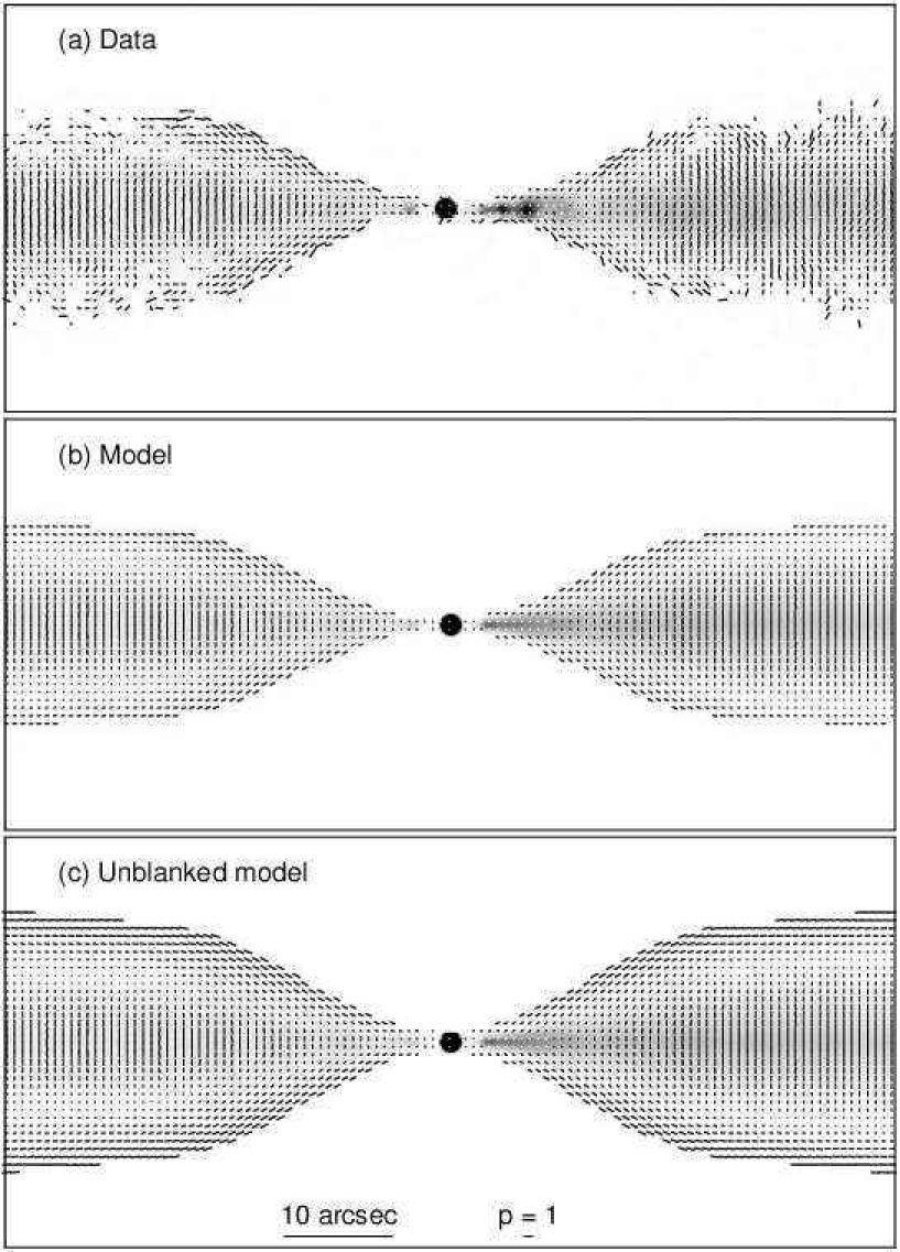
Figure 19: Vectors with lengths proportional to the degree of polarization, $p$, and directions along the apparent magnetic field, superimposed on grey-scales of total intensity. The resolution is 0.75 arcsec and vectors are plotted every 0.6 arcsec. The polarization and angular scales are indicated by the labelled bars in the lowest panel and the areas plotted are the same as those in Figs 12 and 16. (a) data; (b) and (c) model. In panels (a) and (b), vectors are plotted only where $I>5\sigma_{I}$ (Table 2); no blanking has been applied in panel (c).

Although the qualitative difference in width of the transverse apparent field region between the main and counter-jets is reproduced correctly, the model profile is still narrower than the observed one in the outer region of the main jet. The signal-to-noise ratio is low at the edges of the jets, and the model fits should not be taken too seriously there, but the averaged profiles of $Q/I$ shown in Fig. 18(g) suggest that there is a real problem: the longitudinal apparent field predicted by the model at the edges of the main jet (an inevitable consequence of the absence of a radial magnetic-field component) is not seen. In contrast, the corresponding profiles in the counter-jet are accurately reproduced (Fig. 18h). Between $\approx$20 and 60 arcsec from the nucleus, there is significantly more lobe emission at 8.5 GHz around the main jet than the counter-jet (Fig. 9b), so we have examined the possibility that superposition of unrelated lobe emission causes the discrepancy between model and data. The diffuse emission around the main jet has an apparent field transverse to the jet axis, as required to account for the discrepancy, but is not bright enough to produce the observed effect. In order to test whether it is bright enough to affect the profile in Fig. 18(g), we fit and subtracted linear baselines from the $Q$ and $I$ profiles for the jet and counter-jet, using regions between 15 and 20 arcsec from the axis as representative of the lobe emission. The subtracted profiles are indistinguishable from those plotted in Fig. 18(g) and (h) within 12 arcsec of the jet axis. Superposed lobe emission cannot, therefore, be responsible for the discrepancy unless it is significantly enhanced in the vicinity of the jet.

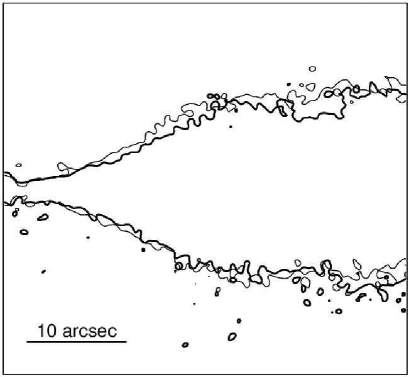
Figure 21: Contours of the 20 $\mu$Jy beam^-1 isophote for the main jet (heavy line) and the counter-jet (light line) rotated by 180^∘ about the core. This figure illustrates that the counter-jet is slightly wider than the main jet in the flaring region. In the outer region, the two isophotes match well on one side, but not on the other (primarily because of a lack of symmetry in the main jet).

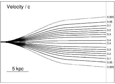
Figure 22: Contours of the model velocity field. The thin contour is at $\beta=0.005$ and the thick contours are at intervals of 0.05 in the range $\beta=$ 0.05 – 0.80.

6 Physical parameters

6.1 Summary of parameters

In this section, all distances in linear units are measured in a plane containing the jet axis (i.e. not projected on the sky). The parameters of the best-fitting model and their approximate uncertainties are given in Table 3.

Table 3: Fitted parameters and error estimates.

Quantity	Symbol	opt	min	max
Angle to line of sight (degrees)	$\theta$	57.9	55.9	61.2
Geometry
Boundary position (kpc)	$r_{0}$	15.8	14.8	16.0
Jet half-opening angle (degrees)	$\xi_{0}$	4.8	2.9	6.9
Half-width of jet at	$x_{0}$	5.2	5.1	5.9
outer boundary (kpc)
Velocity
Boundary positions (kpc)
inner	$\rho_{\rm v_{1}}$	4.6	2.3	5.7
outer	$\rho_{\rm v_{0}}$	5.7	4.6	6.8
On $-$  axis velocities / $c$
inner	$\beta_{1}$	0.8	0.5	$>$0.99
outer	$\beta_{0}$	0.40	0.37	0.47
Fractional velocity at edge of jet
inner	$v_{1}$	0.1	0.0	0.3
outer	$v_{0}$	0.04	0.02	0.08
Emissivity
Boundary positions (kpc)
	$\rho_{\rm e_{\rm in}}$	1.8	1.6	2.0
	$\rho_{\rm e_{\rm knot}}$	2.5	1.9	3.7
	$\rho_{\rm e_{\rm out}}$	8.9	8.4	9.4
On $-$  axis emissivity exponents
	$E_{\rm in}$	2.5	2.0	3.0
	$E_{\rm knot}$	2.1	$-0.4$	4.2
	$E_{\rm mid}$	2.8	2.6	3.1
	$E_{\rm out}$	0.99	0.88	1.12
Fractional emissivity at edge of jet
inner	$e_{1}$	0.8	0.3	2.4
outer	$e_{0}$	0.12	0.10	0.19
B-field
Boundary positions (kpc)
inner	$\rho_{\rm B_{1}}$	0.0	0.0	2.0
outer	$\rho_{\rm B_{0}}$	14.6	12.3	15.9
RMS field ratios
longitudinal/toroidal
inner region axis	$k_{1}^{\rm axis}$	1.7	1.4	2.0
inner region edge	$k_{1}^{\rm edge}$	0.4	0.1	0.6
outer region axis	$k_{0}^{\rm axis}$	0.66	0.57	0.75
outer region edge	$k_{0}^{\rm edge}$	0.0	0.0	0.08

6.2 Geometry and angle to the line of sight

The angle to the line of sight from our model fits is $\theta=58^{+3}_{-2}$ degree. The axis of the nuclear dust ellipse therefore differs from that of the jets by $\approx 15^{\circ}$ in inclination and $\approx 31^{\circ}$ in the plane of the sky (Verdoes Kleijn & de Zeeuw, 2005). The orientation of the dust is such that the counter-jet would be on the receding side of the galaxy if the dust and jet axes are even very roughly aligned. Note, however, that Verdoes Kleijn & de Zeeuw (2005) suggest that dust ellipses such as that seen in 3C 296 are preferentially aligned with the major axes of the galaxies and statistically unrelated to the jet orientations.

The outermost isophote of the jet emission is well fitted by our assumed functional form. The jets flare to a maximum half-opening angle of 26^∘ at a distance of 8.3 kpc from the nucleus, thereafter recollimating. The outer region of conical expansion starts at $r_{0}$ = 15.8 kpc from the nucleus and has a half-opening angle of $\xi_{0}\approx 5^{\circ}$. The outer envelope of the model jet emission is shown in Fig. 23(a). Note that our models fit to faint emission outside the 5$\sigma$ isophote of 20 $\mu$Jy beam^-1 at 0.75-arcsec resolution.

6.3 Velocity

Contours of the derived velocity field are shown in Fig. 22. The positions of the velocity regions, with their uncertainties, and the profiles of velocity along the on-axis and edge streamlines are plotted in Figs 23(b), (d) and (f). The initial on-axis velocity is poorly constrained. The best-fitting value, $\beta_{1}=0.8$, is very uncertain, and the upper limit is unconstrained by our $\chi^{2}$ analysis. The reason for this is that the fractional edge velocity $v_{1}=0.1_{-0.1}^{+0.2}$ is very low: the emission from the main jet close to the brightening point is dominated by slower material. Emission from any high-speed component is Doppler-suppressed and therefore makes very little contribution to the overall $\chi^{2}$. In contrast, after the jets decelerate the on-axis velocity is well-constrained and consistent with a constant value of $\beta_{0}=0.40^{+0.07}_{-0.03}$. The deceleration is extremely rapid in the best-fitting model (Fig. 23d), but the uncertainties in the boundary positions are also large. The low fractional edge velocity at larger distances, $v_{0}=0.04^{+0.06}_{-0.02}$, is required to fit the transverse sidedness-ratio profile (Fig. 15) and is well-determined. The fact that the sidedness ratio is less than unity in places implies that there is some intrinsic asymmetry (Section 5.3), but the qualitative conclusion that the edge velocity is low remains valid.

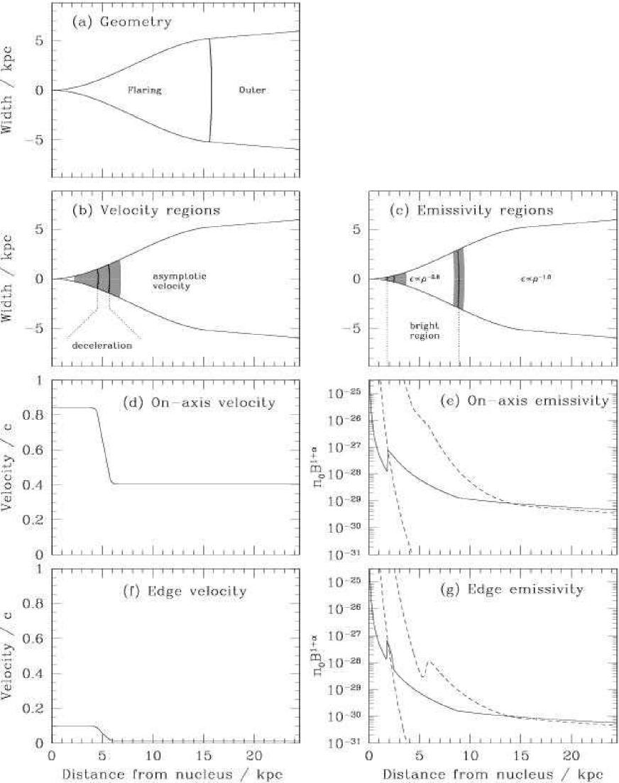
Figure 23: (a) The geometry of the jet, showing the flaring and outer regions. (b) and (c): sketches showing the relative positions of the boundary surfaces between velocity and emissivity regions. The boundaries are defined in Table 4 and their positions for the best fitting model are given in Table 3. The full curves indicate the boundaries and the shaded areas their allowed ranges, also from Table 3. (b) Velocity. The regions of approximately uniform deceleration and asymptotic outer velocity are marked. (c) Emissivity. The region of enhanced emissivity between 1.8 and 9 kpc is indicated. (d) and (e): profiles of intrinsic parameters along the jet axis in the rest frame. (d) the velocity profile. (e) $n_{0}B^{1+\alpha}$ derived from the emissivity, with $n_{0}$ and $B$ in SI units. Solid line: model; dashed line, adiabatic approximation with the magnetic-field structure expected from flux freezing. The latter curve is plotted twice, normalized to the model at 1.8 and 14 kpc from the nucleus, respectively. (f) and (g): profiles of intrinsic parameters along the jet edge in the rest frame. (f) the velocity, (g) the emissivity encoded as in panel (e).

X-ray and ultraviolet emission is detected between 2 and $\approx$10 arcsec from the nucleus (Hardcastle et al., 2005), corresponding to 1.2 – 5.9 kpc in the frame of the jet. This corresponds to the bright part of the flaring region, up to and possibly including the rapid deceleration.

We have evaluated the jet/counter-jet sidedness ratio outside the modelled region by integrating flux densities in boxes of size 10 arcsec along the jet axis and $\pm$15 arcsec transverse to it. The mean ratio drops from $\approx$1.7 between 40 and 70 arcsec from the nucleus to $\approx$1.05 between 70 and 100 arcsec. It is therefore possible that further deceleration to $\beta\la 0.1$ occurs at $\approx$40 kpc in the jet frame. As noted in Section 4.2, however, the jets bend and lobe contamination becomes significant, so we cannot model the velocity variation in this region with much confidence.

6.4 Emissivity

The positions of the emissivity regions, with their uncertainties, and the profiles of emissivity along the on-axis and edge streamlines are plotted in Figs 23(c), (e) and (g). As in all of the FR I sources we have examined so far, the on-axis emissivity profile of 3C 296 is modelled by three power-law sections separated by short transitions. Close to the nucleus, before the brightening point at 1.8 kpc, the power-law index, $E_{\rm in}\approx 2.5\pm 0.5$. The errors on $E_{\rm in}$ are estimated by eye because the jets are faint and any change to the index has very little effect on the value of $\chi^{2}$, even over a small area close to the nucleus. We model the brightening point as a discontinuous increase in emissivity by a factor of $1/g\approx 7$. The short region between 1.8 and 2.5 kpc is introduced primarily to model the first knots in the main and counter-jets; its index is poorly constrained because of our inability to fit the main and counter-jet simultaneously: high values fit the counter-jet knot well but overestimate the main jet brightness; small values have the opposite problem. The main section of the bright jet base from 2.5 – 8.9 kpc is described by a power law of index $E_{\rm mid}=2.8$. This joins smoothly onto the outer region ($E_{\rm out}=1.0$) without the need for a rapid transition. The transverse emissivity profile is fairly flat at the brightening point (albeit with large uncertainties) but evolves to a well-defined Gaussian with a fractional edge emissivity of 0.12 at large distances.

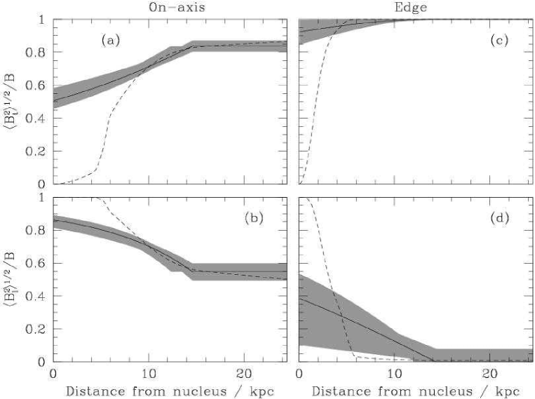
Figure 24: Profiles of magnetic-field components along the axis of the jet (panels a – b) and its edge (panels c – d). The solid lines show the best-fitting model, the shaded areas the uncertainties derived from the limits in Table 3 and the dashed lines the profiles expected for a magnetic field frozen into the flow. The profiles for a passively convected field are normalized to the free model predictions at a distance of 14 kpc from the nucleus. (a) and (c) toroidal; (b) and (d) longitudinal.

6.5 Magnetic-field structure

The inferred magnetic field components are shown as profiles along the on-axis and edge streamlines in Fig. 24 and as false-colour plots in Fig. 25. In the former figure, the shaded areas define the region which the profile could occupy if any one of the six free parameters defining it is varied up to the error quoted in in Table 3. We were able to fit the polarization structure in 3C 296 accurately using a model with only toroidal and longitudinal magnetic-field components. The best fitting model has field-component ratios which vary from the nucleus out to a distance of 14.6 kpc, consistent with the boundary between flaring and outer regions, and thereafter remain constant. The field at the edge of the jet is almost purely toroidal everywhere (Figs 24c, 25a), although there is a marginally significant longitudinal component close to the nucleus (Figs 24d, 25b). On-axis, in contrast, the longitudinal field is initially dominant, but decreases over the flaring region to a smaller, but still significant value at larger distances (Figs 24b, 25b).

We have described the magnetic field structure as disordered on small scales, but anisotropic. A field of this type in an axisymmetric model always generates symmetrical transverse profiles of total intensity, degree of polarization and apparent field position angle. In contrast, a globally-ordered helical field, unless observed at 90^∘ to the line of sight in its rest frame, will always generate asymmetric profiles (Laing, 1981; Laing, Canvin & Bridle, 2006). The observed profiles in 3C 296 (Figs 14, 18) are very symmetrical, even in regions where the longitudinal and transverse field components have comparable amplitudes, so we conclude that a simple, globally-ordered field configuration cannot fit the data. Our calculations would, however, be unchanged if one of the two field components were vector-ordered; in particular, a configuration in which the toroidal component is ordered but the longitudinal one is not would be entirely consistent with our results.

The polarization in the high-signal regions closer to the jet axis requires a mixture of longitudinal and toroidal field components, implying in turn that $p\approx p_{0}$ at the edge of the jet with an apparent field along the jet axis. Our models include this emission, but at a level below the blanking criteria in total intensity and linear polarization at 0.75-arcsec resolution (Fig. 16c). We demonstrated in Section 5.3 that this emission is indeed present and that it has the correct polarization in the counter-jet. In the main jet, contamination by surrounding lobe emission confuses the issue, but there is a real discrepancy (Fig.18g): the observed apparent field remains transverse at the edges. The difference between the main and counter-jets cannot be an effect of aberration as we infer velocities $\beta\ll 1$ in these regions. There must, therefore, be a significant radial field component at the edge of the main jet which is not present at the corresponding location in the counter-jet. Although the low-resolution 8.5-GHz image shown in Fig. 9 gives the impression that the jet might propagate within its associated lobe while the counter-jet is in direct contact with interstellar medium, the L-band images (Fig. 1) show diffuse emission surrounding both jets, so this is unlikely to be the case.

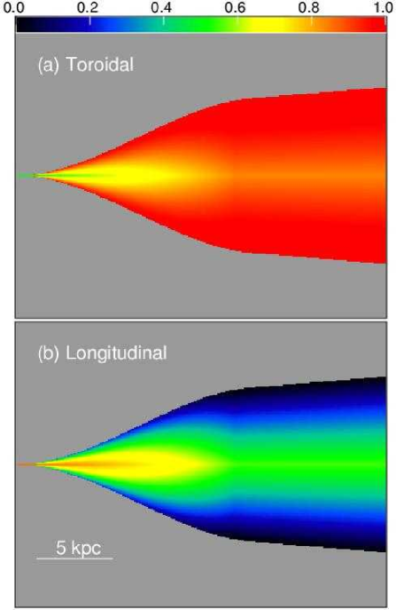
Figure 25: False-colour images of the fractional magnetic-field components. (a) toroidal $\langle B_{t}^{2}\rangle^{1/2}/B$; (b) longitudinal $\langle B_{l}^{2}\rangle^{1/2}/B$. $B=\langle B_{t}^{2}+B_{l}^{2}\rangle^{1/2}$.

6.6 Flux freezing and adiabatic models

Given the assumption of flux freezing in a jet without a transverse velocity gradient, the magnetic field components evolve according to:

$$B_{t} \propto (x\beta\Gamma)^{-1}$$

$$B_{l} \propto x^{-2}$$

in the quasi-one-dimensional approximation, where $x$ is the radius of the jet (Baum et al., 1997). The field-component evolution predicted by these equations is shown by the dashed lines in Fig. 24, arbitrarily normalised to the model values at a distance of 14 kpc from the nucleus. The evolution of the longitudinal/toroidal ratio towards a toroidally-dominated configuration is qualitatively as expected for flux-freezing in an expanding and decelerating flow, but the model shows a much slower decrease. In the absence of any radial field, the ratio should not be affected by shear in the laminar velocity field we have assumed, but the field evolution is clearly more complex than such a simple picture would predict. A small radial field component could still be present, and this would allow the growth of longitudinal field via the strong shear that we infer in 3C 296. We will investigate this process using the axisymmetric adiabatic models developed by Laing & Bridle (2004). A second possibility is that the flow is turbulent in the flaring region. Two-dimensional turbulence (with no velocity component in the radial direction) would lead to amplification of the longitudinal component without generating a large radial component, as required. After the jets recollimate, the model field ratios have constant values on a given streamline, consistent with the variation expected from flux freezing in a very slowly expanding flow (Fig. 24). Note, however, the problems in fitting the main jet polarization at large distances from the axis (Section 6.5).

If the radiating electrons suffer only adiabatic losses, the emissivity is:

$$\epsilon\propto(x^{2}\beta\Gamma)^{-(1+2\alpha/3)}B^{1+\alpha}$$

in the quasi-one-dimensional approximation (Baum et al., 1997; Laing & Bridle, 2004). $B$ can be expressed in terms of the parallel-field fraction $f=\langle B_{l}^{2}\rangle^{1/2}/B$ and the radius $\bar{x}$, velocity $\bar{\beta}$ and Lorentz factor $\bar{\Gamma}$ at some starting location using equation 8 of Laing & Bridle (2004):

$$B\propto\left[f^{2}\left(\frac{\bar{x}}{x}\right)^{4}+(1-f^{2})\left(\frac{\bar{\Gamma}\bar{\beta}\bar{x}}{\Gamma\beta x}\right)^{2}\right]^{1/2}$$

The resulting profiles for the on-axis and edge streamlines are plotted as dashed lines in Fig. 23(e) and (g), normalized to the model values at the brightening point (1.8 kpc) and 14 kpc. Their slopes are grossly inconsistent with the model emissivity in the flaring region, but match well beyond $\sim$14 kpc – essentially where the jet recollimates at $r_{0}$ = 15.8 kpc.

6.7 Arcs

As pointed out in Section 3.1, there are discrete, narrow features (“arcs”) in the brightness distributions of both jets in 3C 296. Strikingly similar structures are seen in the jets of 3C 31 (LB), as shown in Fig. 26. In both sources, the arcs have systematically different shapes in the main and counter-jets: centre-brightened arcs with well-defined intensity gradients near the jet axis [type (i)] are found in the main jets of both sources and in the outer counter-jet of 3C 296, while more elongated arcs with well-defined intensity gradients near the jet edges [type (ii)] are found in both counter-jets. We will present models of the arc structures elsewhere: here we demonstrate that relativistic aberration can plausibly account for the systematic difference.

Suppose that an arc is a thin, axisymmetric shell of enhanced emissivity, concave towards the nucleus, and that at any point its speed is roughly that of the local average flow. Close to the centre-line of the jet, the shell can be approximated as a planar sheet of material orthogonal to the axis in the observed frame. Aberration causes a moving object to appear at the angle to the line of sight appropriate to the rest frame of the flow (Penrose, 1959; Terrell, 1959). For the the normals to the sheets in the main and counter-jets these angles are $\theta_{\rm j}^{\prime}$ and $\theta_{\rm cj}^{\prime}$, where:

$$\sin\theta_{\rm j}^{\prime} = \sin\theta[\Gamma(1-\beta\cos\theta)]^{-1}$$

$$\sin\theta_{\rm cj}^{\prime} = \sin\theta[\Gamma(1+\beta\cos\theta)]^{-1}$$

just as in Section 4.2.

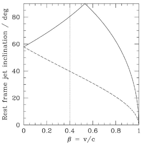
Figure 27: The angle to the line of sight in the fluid rest frame for a vector parallel to the flow in the observed frame plotted against $\beta=v/c$. The angle between the jet axis and the line of sight is $\theta=58^{\circ}$, as we infer for 3C 296. Full line: main jet; dashed line: counter-jet. The vertical dotted line marks the on-axis velocity of $\beta=0.4$ we derive for the outer parts of the modelled region in 3C 296.

In 3C 296, the arcs are visible as far as $\approx$90 arcsec from the nucleus – outside the region we model – so we do not have a direct measure of the average velocity field in their vicinity. Given that our model indicates a roughly constant velocity on-axis from 10 – 40 arcsec from the nucleus we will assume for the purposes of a rough estimate that the parameters at the outer edge of the model approximate the average flow parameters near the arcs between 40 and 70 arcsec, where the mean jet/counter-jet sidedness ratio remains significantly larger than unity. In Fig. 27 we plot $\theta_{\rm j}^{\prime}$ and $\theta_{\rm cj}^{\prime}$ against $\beta$ for $\theta=58^{\circ}$ (Table 3). For a velocity $\beta=\beta_{0}=0.40$, the angles to the line of sight in the fluid rest frame are $\theta_{\rm j}^{\prime}=80^{\circ}$ and $\theta_{\rm cj}^{\prime}=40^{\circ}$ (the main jet is close to the maximum boost condition $\beta=\cos\theta$ which corresponds to edge-on emission in the rest frame). A sheet of enhanced emissivity which is normal to the flow on the jet axis is therefore observed nearly edge-on in the main jet, appearing narrow, with a high brightness gradient. In the counter-jet, on the other hand, the same sheet would appear to be significantly rotated about a line perpendicular to the jet axis in the plane of the sky and therefore less prominent both in intensity and in brightness gradient. Close to the edges of the jets, however, the model flow velocities are essentially zero, so the effects of aberration should be negligible. If the shells are roughly tangential to the surface, then we expect to see narrow brightness enhancements orientated parallel to the edges in both jets.

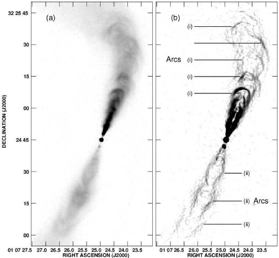
Figure 26: 8.5-GHz images of the jets in the FR  radio galaxy 3C 31 (LB) with grey-scale ranges chosen to emphasise the arc structures, as in the equivalent plots for 3C 296 (Fig. 2). (a) Total intensity. (b) Sobel-filtered $I$. The resolution is 0.75 arcsec FWHM. The arcs are labelled with their types as defined in Section 6.7 (except for the fourth from the nucleus in the main jet, which appears to be associated with the bend in the jet and is clearly not axisymmetric).

This picture provides a reasonable qualitative description of the differences in arc structure for the main and counter-jets in 3C 296 within $\approx$70 arcsec of the nucleus (Fig. 2). The evolution of the mean jet/counter-jet ratio suggests that the jets become sub-relativistic at larger distances (Section 6.3) and this may explain why we see type (i) arcs in both jets between 70 and 90 arcsec.

The hypothesis that the main difference in appearance of the arcs between the main and counter-jets is an effect of differential relativistic aberration also allows us to predict that differences should be observed between main and counter-jet arcs in other FR I sources if they are orientated at moderate angles to the line of sight. This explains why we observe systematic differences in the arcs of 3C 31, which has similar model parameters to 3C 296 (Fig. 26, LB), but we would not expect differences between the main and counter-jet arcs if $\theta_{\rm j}^{\prime}$ and $\theta_{\rm cj}^{\prime}$ are similar. The latter condition holds if the jets are close to the plane of the sky (e.g. 3C 449 and PKS 1333-33; Feretti et al. 1999; Killeen et al. 1986) or slow (e.g. the outer region of B2 0326+39; CL). It will therefore be interesting to search for arcs in deep images of these sources.

7 Comparison between sources

We have modelled five FR I sources: 3C 31 (LB), B2 0326+39, B2 1553+24 (CL), NGC 315 (CLBC) and 3C 296 (this paper). We will compare and contrast their properties in detail elsewhere, but in this section we summarize their similarities and differences and draw attention to a few potential problems with our approach.

7.1 Similarities

The five FR I sources we have studied in detail so far all exhibit the following similarities:

1. A symmetrical, axisymmetric, decelerating jet model fits the observed brightness and polarization distributions and asymmetries well.

2. The outer boundaries of the well-resolved parts of the jets can be divided into two main regions: a flaring region with a rapidly increasing expansion rate followed by recollimation and an outer region with a uniform expansion rate.

3. Close to the nucleus, the on-axis velocity is initially consistent with $\beta\approx 0.8$. On-axis, rapid deceleration then occurs over distances of 1 – 10 kpc, after which the velocity either stays constant or decreases less rapidly.

4. All except B2 1553+24 have low emissivity at the base of the “flaring” region, so even the main jet is initially very faint (this region may be present but unresolved in B2 1553+24).

5. The faint region ends at a “brightening point” where the emissivity profile flattens suddenly or even increases. This, coupled with the rapid expansion of the jets, leads to a sudden increase in surface brightness in the main jets (not necessarily in the counter-jets, whose emission is Doppler suppressed).

6. The brightening point is always before the start of rapid deceleration, which in turn is completed before the jets recollimate.

7. Immediately after the brightening point, all of the jets contain bright substructure with complex, non-axisymmetric features which we cannot model in detail.

8. Optical/ultraviolet or X-ray emission has been detected in all of the jets observed so far with HST or Chandra (results for B2 0326+39 are not yet available). High-energy emission is associated with the bright regions of the main jets before the onset of rapid deceleration in all cases, and also with the faint inner region in 3C 31.

9. The longitudinal emissivity profile may be represented by three power-law segments separated by short transitions. The indices of the power laws decrease with distance from the nucleus.

10. All of the jets are intrinsically centre-brightened, with fractional emissivities at their edges $\approx$0.1 – 0.5 where these are well-determined.

11. On average, the largest single magnetic field component is toroidal. The longitudinal component is significant close to the nucleus but decreases with distance. The radial component is always the smallest of the three.

12. For those sources we have fit with functional forms allowing variation of field-component ratios across the jets (3C 31, NGC 315 and 3C 296), we find that the toroidal component is stronger relative to the longitudinal component at the edge of the jet (this is likely to be true for the other two sources).

13. The evolution of the field component ratios along the jets before they recollimate is not consistent with flux freezing in a laminar flow, which requires a much more rapid transition from longitudinal to transverse field than we infer. A possible reason for this is two-dimensional turbulence (with no radial velocity component) in the flaring regions. After recollimation, flux freezing is consistent with our results.

14. The inferred evolution of the radial/toroidal field ratio (in those sources where the radial component is non-zero) is qualitatively inconsistent with flux freezing even if shear in a laminar velocity field is included.

15. The quasi-one-dimensional adiabatic approximation (together with flux freezing) is grossly inconsistent with the emissivity evolution required by our models before the jets decelerate and recollimate. Earlier attempts to infer fractional changes in velocity from surface-brightness profiles (Fanti et al., 1982; Bicknell, 1984, 1986; Bicknell et al., 1990; Baum et al., 1997; Bondi et al., 2000), therefore required much more rapid deceleration than we deduce in these regions.

16. After deceleration and recollimation, the emissivity evolution along the jets is described quite well by flux freezing and a quasi-one-dimensional adiabatic approximation (our analysis does not cover this region in NGC 315). As relativistic effects are slight, the brightness evolution in the outer regions of 3C 296, B2 0326+39 and B2 1553+24 is quite close to the constant-speed, perpendicular-field prediction originally derived by Burch (1979). Previous estimates of fractional velocity changes derived on the adiabatic assumption [references as in (xv), above] are likely to be more reliable on these larger scales.

7.2 Differences

3C 296 exhibits the following differences from the other sources:

1. The transverse velocity profile falls to a low fractional value $\la 0.1$ at the edge of the jets in 3C 296, whereas all the other sources are consistent with an edge/on-axis velocity ratio $\approx$0.7 everywhere, and also with a top-hat velocity profile at the brightening point. This could be related to the differences in lobe structure: as noted earlier, 3C 296 is the only source we have observed with a bridged twin-jet structure. Its jets may then be embedded (almost) completely within the lobes rather than propagating in direct contact with the interstellar medium of the host galaxy. Modelling of other bridged FR I sources would then be expected to show similarly low edge velocities. Whether the lower-velocity material is best regarded as part of the jets or the lobes (and, indeed, whether this distinction is meaningful) remains unclear.

2. Some support for the idea of an interaction between jets and lobes comes from our detection of anomalous (i.e. inconsistent with our model predictions) polarization at the edges of the main jet in its outer parts. We have argued that this cannot be a simple superposition of unrelated jet and lobe emission.

3. Rapid deceleration is complete before the end of the bright region in 3C 296. In contrast, the bright region ends within the deceleration zone for B2 0326+39, B2 1553+24 and NGC 315 and the end of the bright region roughly coincides with the end of rapid deceleration in 3C 31.

4. When deciding where in the jets our hypothesis of intrinsic symmetry first becomes inappropriate, we have successfully used the criterion that the jets must remain straight while selecting the region to be analysed. In 3C 296 however there are hints of intrinsic asymmetries on a still smaller scale because the counter-jet appears to be slightly wider than the main jet in the flaring region.

Our results are generally consistent with the conclusions of a statistical study of a larger sample of FR I sources with jets (Laing et al., 1999), but the velocity range at the brightening point derived from the distribution of jet/counter-jet ratios assuming an isotropic sample has a maximum $\beta_{\rm max}\approx 0.9$ and a minimum in the range $0.3\ga\beta_{\rm min}\ga 0$. Such a range would be expected if low edge velocities (as in 3C 296) are indeed typical of bridged twin-jet sources, since these form the majority of the sample (Parma et al., 1996).

8 Summary

We have made deep, 8.5-GHz images of the nearby FR I radio galaxy 3C 296 with the VLA at resolutions ranging from 0.25 to 5.5 arcsec FWHM, revealing new details of its twin jets. In particular we see several thin, discrete brightness enhancements (“arcs”) in both jets. These appear to have systematically different morphologies in the main and counter-jets. A comparison with lower-frequency images from archive data shows that the flat-spectrum jets are surrounded by a broad sheath of steeper-spectrum diffuse emission, possibly formed by a backflow of radiating plasma which has suffered significant synchrotron losses as in models of FR II sources. The spectral index of the jets initially flattens slightly with distance from the nucleus (from $\alpha\approx 0.62$ to $\alpha\approx 0.53$) as in other FR I jets. We have also imaged the Faraday rotation and depolarization over the source. The counter-jet is more depolarized than the main jet, but the differences in depolarization and Faraday rotation variance between the two lobes are small. The rms fluctuations in rotation measure are larger close to the nucleus in both lobes.

We have shown that many features of the synchrotron emission from the inner $\pm$40 arcsec of the jets in 3C 296 can be fit accurately and self-consistently on the assumption that they are intrinsically symmetrical, axisymmetric, decelerating, relativistic flows. The functional forms we use for the model are similar to those developed in our earlier work, as are most of the derived physical parameters. In this sense, a strong family resemblance is emerging between the physical properties that we derive for the outflows in these FR I sources.

Geometry

The jets can be divided into a flaring region, whose radius $x$ is well fitted by the expression $x=a_{2}z^{2}+a_{3}z^{3}$, where $z$ is the distance from the nucleus along the axis, and a conical outer region. We infer an angle to the line of sight of $58^{+3}_{-2}$ degree. The boundary between the two regions is then at 15.8 kpc from the nucleus.

Velocity structure

Where the jets first brighten, their on-axis velocity is $\beta\approx 0.8$, but this value is poorly constrained. Rapid deceleration occurs around 5 kpc to an on-axis velocity of $\beta=0.40^{+0.07}_{-0.03}$ which thereafter remains constant. 3C 296 differs from all of the other objects we have studied in having a very low velocity (essentially consistent with 0) at the edges of its jets.

Emissivity

The longitudinal profile of rest-frame emissivity is modelled as three principal power-law sections $\epsilon\propto\rho^{-E}$ with indices of $E=2.5$ (0 – 1.8 kpc), $2.8$ (2.5 – 8.9 kpc) and $1.0$ (8.9 – 24.5 kpc, the end of the modelled region). The first two regions are separated by a short transition zone in which the emissivity increases discontinuously by a factor of $\approx$7 and then has a power-law slope $\sim$2.1 (1.8 – 2.5 kpc; representing the first knots in the main and counter-jets). The rest-frame emissivity is centre-brightened.

Magnetic-field configuration

We model the magnetic field as disordered, but anisotropic, with toroidal and longitudinal components, but our results are equally consistent with an ordered toroidal component. We rule out a globally-ordered helical field. The ratio of longitudinal to toroidal field decreases with distance from the nucleus; the toroidal component is also more dominant at the edges of the jets.

Flux freezing

The field-component evolution is qualitatively consistent with flux freezing, but much slower than expected in the flaring region, where the adiabatic approximation also fails to fit the emissivity variation. In the outer region, after the jets decelerate, the adiabatic approximation is a reasonable fit.

Arc asymmetry

If the arcs are narrow shells of enhanced emissivity moving with the underlying flow, then the differences in their appearance in the main and counter-jets can be understood as the effect of relativistic aberration, as required for a fully self-consistent model of the jets.

Appendix A Functional forms for velocity, emissivity and field ordering

In Table 4, we give for reference the functional forms for the spatial variations of velocity, emissivity and magnetic-field ordering used in this paper. They are identical to those used by CLBC except for the elimination of any radial field component and a slight change to the form of the longitudinal emissivity profile. We use the streamline coordinate system $(\rho,s)$ In the outer region, the streamline index $s=\xi/\xi_{0}$, where $\xi$ is the angle between the (straight) streamline and the axis. In the flaring region, the distance of a streamline from the jet axis at a distance $z$ from the nucleus is $x(z,s)=a_{2}(s)z^{2}+a_{3}(s)z^{3}$, the coefficients being defined by continuity of $x(s)$ and its first derivative across the boundary between the outer and flaring regions. The coordinate $\rho$ increases monotonically along a streamline and is defined by:

$$\rho = \frac{zr_{0}\sin\xi_{0}}{r_{0}\sin\xi_{0}+x_{0}(\cos\xi_{0}s-1)}\hskip 71.13188pt\rho<r_{0}$$

$$\rho = \frac{z\sin\xi_{0}+(x_{0}-r_{0}\sin\xi_{0})(1-\cos\xi_{0}s)}{\sin\xi_{0}\cos\xi_{0}s}\hskip 28.45274pt\rho\geq r_{0}$$

On-axis ($s=0$), $\rho=z$ in both regions.

Table 4: Functional forms of the velocity $\beta$, emissivity $\epsilon$ and longitudinal/toroidal magnetic-field ratios $k$ in the streamline coordinate system $(\rho,s)$. Column 4 lists the parameters which may be optimized, for comparison with Table 3.

Quantity	Functional form	Range	Free parameters
Velocity field
$\beta(\rho,s)$	$\beta_{1}\exp(-s^{2}\ln v_{1})$
	$-\left[\frac{\beta_{1}\exp(-s^{2}\ln v_{1})-\beta_{0}\exp(-s^{2}\ln v_{0})}{10}\right]\exp[c_{1}(\rho-\rho_{\rm v_{1}})]$	$\rho<\rho_{\rm v_{1}}$	Distances $\rho_{\rm v_{1}}$, $\rho_{\rm v_{0}}$
	$c_{2}+c_{3}\rho$	$\rho_{\rm v_{1}}\leq\rho\leq\rho_{\rm v_{0}}$	Velocities $\beta_{1}$, $\beta_{0}$
	$\beta_{0}\exp(-s^{2}\ln v_{0})$
	$+\left[\frac{\beta_{1}\exp(-s^{2}\ln v_{1})-\beta_{0}\exp(-s^{2}\ln v_{0})}{10}\right]\exp[c_{4}(\rho_{\rm v_{0}}-\rho)]$	$\rho>\rho_{\rm v_{0}}$	Fractional edge velocities $v_{1}$, $v_{0}$
Emissivity
$\epsilon(\rho,s)$	$~{}~{}~{}g\left(\frac{\rho}{\rho_{\rm e_{\rm in}}}\right)^{-E_{\rm in}}$	$\rho\leq\rho_{\rm e_{\rm in}}$	Distances $\rho_{\rm e_{\rm in}}$, $\rho_{\rm e_{\rm knot}}$, $\rho_{\rm e_{\rm out}}$
	$\left(\frac{\rho}{\rho_{\rm e_{\rm in}}}\right)^{-E_{\rm knot}}\exp\left[-s^{2}\ln\left(e_{\rm in}+(e_{0}-e_{\rm in})\left(\frac{\rho-\rho_{\rm e_{\rm in}}}{\rho_{\rm e_{\rm knot}}-\rho_{\rm e_{\rm in}}}\right)\right)\right]$	$\rho_{\rm e_{\rm in}}<\rho\leq\rho_{\rm e_{\rm knot}}$	Indices $E_{\rm in}$, $E_{\rm knot}$, $E_{\rm mid}$, $E_{\rm out}$
	$d_{1}\left(\frac{\rho}{\rho_{\rm e_{\rm knot}}}\right)^{-E_{\rm mid}}\exp(-s^{2}\ln e_{0})$	$\rho_{\rm e_{\rm knot}}<\rho\leq\rho_{\rm e_{\rm out}}$	Fractional edge emissivities $e_{1}$, $e_{0}$
	$d_{2}\left(\frac{\rho}{\rho_{\rm e_{\rm out}}}\right)^{-E_{\rm out}}\exp(-s^{2}\ln e_{0})$	$\rho>\rho_{\rm e_{\rm out}}$	Fractional jump at inner boundary, $g$
Longitudinal/toroidal field ratio
$k(\rho,s)$	$k_{1}^{\rm axis}+s(k_{1}^{\rm edge}-k_{1}^{\rm axis})$	$\rho\leq\rho_{\rm B_{1}}$	Ratios $k_{1}^{\rm edge}$, $k_{0}^{\rm edge}$, $k_{1}^{\rm axis}$, $k_{0}^{\rm axis}$
	$k^{\rm axis}+s(k^{\rm edge}-k^{\rm axis})$	$\rho_{\rm B_{1}}<\rho<\rho_{\rm B_{0}}$	Distances $\rho_{\rm B_{1}}$, $\rho_{\rm B_{0}}$
	where  $k^{\rm axis}=k_{1}^{\rm axis}+(k_{0}^{\rm axis}-k_{1}^{\rm axis})\left(\frac{\rho-\rho_{\rm B_{1}}}{\rho_{\rm B_{0}}-\rho_{\rm B_{1}}}\right)$
	$k^{\rm edge}=k_{1}^{\rm edge}+(k_{0}^{\rm edge}-k_{1}^{\rm edge})\left(\frac{\rho-\rho_{\rm B_{1}}}{\rho_{\rm B_{0}}-\rho_{\rm B_{1}}}\right)$
	$k_{0}^{\rm axis}+s(k_{0}^{\rm edge}-k_{0}^{\rm axis})$	$\rho\geq\rho_{\rm B_{0}}$

References

- (1)
- Baum et al. (1997) Baum S.A., O’Dea C.P., Giovannini G., Biretta J., Cotton W.B., de Koff S., Feretti L., Golombek D., Lara L., Macchetto F.D., Miley G.K., Sparks W.B., Venturi T., Komissarov S.S., 1997, ApJ, 483, 178 (erratum ApJ, 492, 854)
- Begelman et al. (1984) Begelman M.C., Blandford R.D., Rees M.J., 1984, Rev. Mod. Phys., 56, 255
- Bicknell (1984) Bicknell, G.V., 1984, ApJ, 286, 68
- Bicknell (1986) Bicknell, G.V., 1986, ApJ, 305, 109
- Bicknell (1994) Bicknell, G.V., 1994, ApJ, 422, 542
- Bicknell et al. (1990) Bicknell G.V., de Ruiter H.R., Parma P., Morganti R., Fanti, R., 1982, ApJ, 354, 98
- Biretta, Zhou & Owen (1995) Biretta J.A., Zhou F., Owen F.N., 1995, ApJ, 447, 582
- Birkinshaw, Laing & Peacock (1981) Birkinshaw M., Laing R.A., Peacock J.A., 1981, MNRAS, 197, 253
- Bondi et al. (2000) Bondi M., Parma P., de Ruiter H.R., Laing R.A., Fomalont E.B., 2000, MNRAS, 314, 11
- Bowman, Leahy & Komissarov (1996) Bowman M., Leahy J. P., Komissarov S. S., 1996, MNRAS, 279, 899
- Bridle (1982) Bridle, A.H. 1982, in Extragalactic Radio Sources, eds Heeschen D.S., Wade C.M., IAU Symp. 97, Kluwer, Dordrecht, p. 121
- Burch (1979) Burch S.F., 1979, MNRAS, 187, 187
- Canvin & Laing (2004) Canvin J.R., Laing R.A., 2004, MNRAS, 350, 1342 (CL)
- Canvin et al. (2005) Canvin, J.R., Laing, R.A., Bridle, A.H., Cotton, W.D., 2005, MNRAS, 363, 1223 (CLBC)
- Chiaberge, Capetti & Celotti (1999) Chiaberge M., Capetti A., Celotti A., 1999, A&A 349, 77
- de Koff et al. (2000) de Koff S., Best P., Baum S.A., Sparks W., Röttgering H., Miley G., Golombek D., Macchetto F., Martel A., 2000, ApJS, 129, 33
- Dineen & Coles (2005) Dineen P., Coles P., 2005, MNRAS, 362, 403
- Fanaroff & Riley (1974) Fanaroff B.L., Riley J.M., 1974, MNRAS, 167, 31p
- Fanti et al. (1982) Fanti R., Lari C., Parma P., Bridle A.H., Ekers R.D., Fomalont E.B, 1982, A&A, 110, 169
- Feretti et al. (1999) Feretti L., Perley R., Giovannini G., Andernach H., 1999, A&A, 341, 29
- Garrington et al. (1996) Garrington S.T., Holmes G.F., Saikia D.J., 1996, in Extragalactic Radio Sources, eds Ekers R.D., Fanti C., Padrielli L., IAU Symp. 175, Kluwer, Dordrecht, p. 397
- Giovannini et al. (2001) Giovannini G., Cotton W.D., Feretti L., Lara L., Venturi T., 2001, ApJ, 552, 508
- Giovannini et al. (2005) Giovannini G., Taylor G.B., Feretti L., Cotton W.D., Lara L., Venturi T., 2005, ApJ, 618, 635
- Hardcastle et al. (1997) Hardcastle M.J., Alexander P., Pooley G.G., Riley J.M., 1997, MNRAS, 288, L1
- Hardcastle & Worrall (1999) Hardcastle M.J., Worrall D.M., 1999, MNRAS, 309, 969
- Hardcastle et al. (2003) Hardcastle M.J., Worrall D.M., Kraft R.P., Forman W.R., Jones C., Murray S.S., 2003, ApJ, 593, 169
- Hardcastle et al. (2005) Hardcastle M.J., Worrall D.M., Birkinshaw M., Laing R.A., Bridle A.H., 2005, MNRAS, 358, 843
- Katz-Stone & Rudnick (1997) Katz-Stone D.M., Rudnick L., 1997, ApJ, 488, 146
- Katz-Stone et al. (1999) Katz-Stone D.M., Rudnick L., Butenhoff C., O’Donoghue A.A., 1999, ApJ, 516, 716
- Killeen et al. (1986) Killeen N.E.B., Bicknell G.V., Ekers R.D., 1986, ApJ, 302, 306
- Komissarov (1994) Komissarov S.S., 1994, MNRAS, 269, 394
- Königl (1980) Königl, A., 1980, Phys. Fluids, 23, 1083
- Laing (1981) Laing R.A., 1981, ApJ, 248, 87
- Laing (1988) Laing R.A., 1988, Nature, 331, 149
- Laing (1996) Laing R.A., 1996, in Extragalactic Radio Sources, eds Ekers R.D., Fanti C., Padrielli L., IAU Symp. 175, Kluwer, Dordrecht, p. 147
- Laing & Bridle (2002a) Laing R.A., Bridle A.H., 2002a, MNRAS, 336, 328 (LB)
- Laing & Bridle (2002b) Laing R.A., Bridle A.H., 2002b, MNRAS, 336, 1161
- Laing & Bridle (2004) Laing R.A., Bridle A.H., 2004, MNRAS, 348, 1459
- Laing, Canvin & Bridle (2006) Laing R.A., Canvin J.R., Bridle A.H., 2006, AN, 327, 523
- Laing et al. (2006) Laing R.A., Canvin J.R., Cotton W.D., Bridle A.H., 2006, MNRAS, 368, 48
- Laing et al. (1999) Laing R.A., Parma P., de Ruiter H.R., Fanti, R., 1999, MNRAS, 306, 513
- Laing & Peacock (1980) Laing R.A., Peacock J.A., 1980, MNRAS, 190, 903
- Leahy & Perley (1991) Leahy J.P., Perley R.A., 1991, AJ, 102, 537
- Leahy, Pooley & Riley (1986) Leahy J.P., Pooley G.G., Riley J.M., 1986, MNRAS, 222, 753
- Martel et al. (1999) Martel A., et al. 1999, ApJS, 122, 81
- Miller et al. (2002) Miller N.A., Ledlow M.J., Owen F.N., Hill J.M., 2002, AJ, 123, 3018
- Miller et al. (1999) Miller N.A., Owen F.N., Burns J.O., Ledlow M.J., Voges W., Hill J.M., 1999, AJ, 118, 1988
- Morganti et al. (1997) Morganti R., Parma P., Capetti A., Fanti R., de Ruiter H.R., 1997, A&A, 326, 919
- Parma et al. (1996) Parma, P., De Ruiter, H.R., Fanti, R., 1996, in Extragalactic Radio Sources, eds Ekers R.D., Fanti C., Padrielli L., IAU Symp. 175, Kluwer, Dordrecht, p. 137
- Penrose (1959) Penrose R., 1959, Proc. Camb. Phil. Soc., 55, 137
- Phinney (1983) Phinney E. S., 1983, Ph.D. Thesis, University of Cambridge
- Pratt (1991) Pratt, W.K., 1991, Digital Image Processing, Wiley, New York
- Simard-Normandin, Kronberg & Button (1981) Simard-Normandin M., Kronberg P.P., Button S., 1981, ApJS, 45, 97
- Taylor & Perley (1993) Taylor G.B., Perley R.A., 1993, ApJ, 416, 554
- Terrell (1959) Terrell J., 1959, Phys. Rev., 116, 1041
- Taylor, Ulvestad & Perley (2004) Taylor, G. B., Ulvestad, J.S., Perley, R.A., 2004, The Very Large Array Observational Status Summary, NRAO, Socorro, http://www.vla.nrao.edu/astro/guides/vlas/current/
- Urry & Padovani (1995) Urry C. M., Padovani P., 1995, PASP, 107, 803
- Verdoes Kleijn & de Zeeuw (2005) Verdoes Kleijn G., de Zeeuw P.T., 2005, A&A, 435, 43
- Wardle & Kronberg (1974) Wardle J.F.C., Kronberg P.P., 1974, ApJ, 194, 249