Particle Accelerator in Pulsar Magnetospheres: Super Goldreich-Julian Current with Ion Emission from the Neutron Star Surface

Abstract

We investigate the self-consistent electrodynamic structure of a particle accelerator in the Crab pulsar magnetosphere on the two-dimensional poloidal plane, solving the Poisson equation for the electrostatic potential together with the Boltzmann equations for electrons, positrons and gamma-rays. If the trans-field thickness of the gap is thin, the created current density becomes sub-Goldreich-Julian, giving the traditional outer-gap solution but with negligible gamma-ray luminosity. As the thickness increases, the created current increases to become super-Goldreich-Julian, giving a new gap solution with substantially screened acceleration electric field in the inner part. In this case, the gap extends towards the neutron star with a small-amplitude positive acceleration field, extracting ions from the stellar surface as a space-charge-limited flow. The acceleration field is highly unscreened in the outer magnetosphere, resulting in a gamma-ray spectral shape which is consistent with the observations.

1 Introduction

The Energetic Gamma Ray Experiment Telescope (EGRET) aboard the Compton Gamma Ray Observatory has detected pulsed signals from at least six rotation-powered pulsars (e.g., for the Crab pulsar, Nolan et al. 1993, Fierro et al. 1998). Since interpreting $\gamma$-rays should be less ambiguous compared with reprocessed, non-thermal X-rays, the $\gamma$-ray pulsations observed from these objects are particularly important as a direct signature of basic non-thermal processes in pulsar magnetospheres, and potentially should help to discriminate among different emission models.

The pulsar magnetosphere can be divided into two zones (fig. 1): The closed zone filled with a dense plasma corotating with the star, and the open zone in which plasma flows along the open field lines to escape through the light cylinder. The last-open field lines form the border of the open magnetic field line bundle. In all the pulsar emission models, particle acceleration and the resultant photon emissions take place within this open zone.

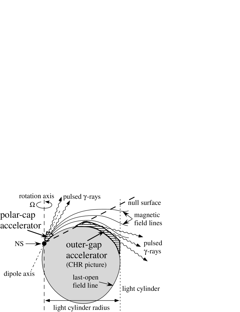
Figure 1: Schematic figure (sideview) of the two representative accelerator models. The small filled circle represents the neutron star

On the spinning neutron star surface, an electro-motive force, $\mbox{EMF}\approx\Omega^{2}B_{\ast}r_{\ast}^{3}/c^{2}\approx 10^{16.5}$ V, is exerted from the magnetic pole to the rim of the polar cap. In this paper, we assume that both the spin and magnetic axes reside in the same hemisphere; that is, $\mbox{\boldmath$\Omega$}\cdot\mbox{\boldmath$\mu$}>0$, where $\Omega$ represents the rotation vector, and $\mu$ the stellar magnetic moment vector. This strong EMF causes the magnetospheric currents that flow outwards in the lower latitudes and inwards near the magnetic axis (left panel in fig. 2). The return current is formed at large-distances where Poynting flux is converted into kinetic energy of particles or dissipated (Shibata 1997).

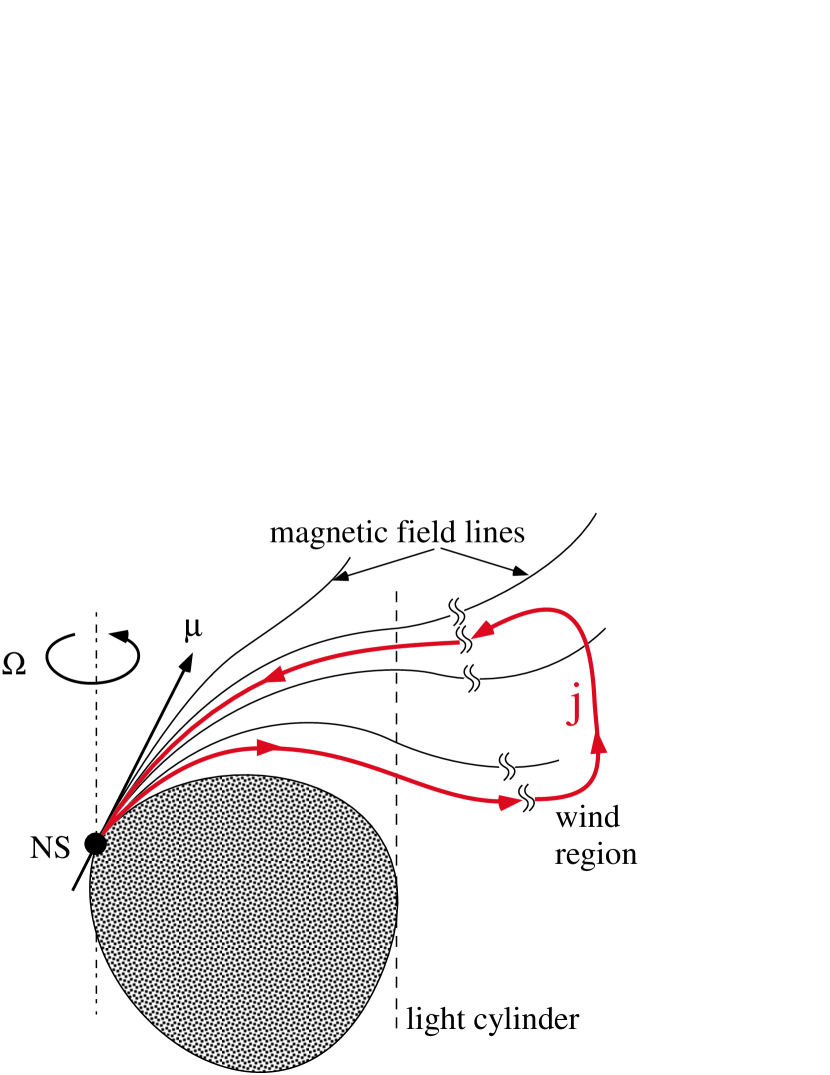
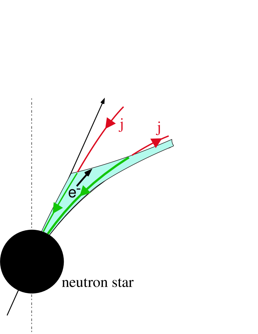
Figure 2: Schematic picture of electric current in the pulsar magnetosphere. Left: Global electric current due to the EMF exerted on the spinning neutron star surface when $\mbox{\boldmath$\Omega$}\cdot\mbox{\boldmath$\mu$}>0$. Right: Current (downward arrows) derived in the inner-slot-gap (shaded region).

Attempts to model the particle accelerator have traditionally concentrated on two scenarios: Polar-cap models with emission altitudes of $\sim 10^{4}$cm to several neutron star radii over a pulsar polar cap surface (Harding, Tademaru, & Esposito 1978; Daugherty & Harding 1982, 1996; Dermer & Sturner 1994; Sturner, Dermer, & Michel 1995), and outer-gap models with acceleration occurring in the open zone located near the light cylinder (Cheng, Ho, & Ruderman 1986a,b, hereafter CHR86a,b; Chiang & Romani 1992, 1994; Romani and Yadigaroglu 1995). Both models predict that electrons and positrons are accelerated in a charge depletion region, a potential gap, by the electric field along the magnetic field lines to radiate high-energy $\gamma$-rays via the curvature and inverse-Compton (IC) processes.

In the outer magnetosphere picture of Romani (1996), he estimated the evolution of high-energy flux efficiencies and beaming fractions to discuss the detection statistics, by considering how pair creation on thermal surface flux can limit the acceleration zones. Subsequently, Cheng, Ruderman and Zhang (2000, hereafter CRZ00) developed a three-dimensional outer magnetospheric gap model, self-consistently limiting the gap size by pair creation from collisions of thermal photons from the polar cap that is heated by the bombardment of gap-accelerated charged particles. The outer gap models of these two groups have been successful in explaining the observed light curves, particularly in reproducing the wide separation of the two peaks commonly observed from $\gamma$-ray pulsars (Kanbach 1999; Thompson 2001), without invoking a very small inclination angle. In these outer gap models, they consider that the gap extends from the null surface, where the Goldreich-Julian charge density vanishes, to the light cylinder, beyond which the velocity of a co-rotating plasma would exceed the velocity of light, adopting the vacuum solution of the Poisson equation for the electrostatic potential (CHR86a).

However, it was analytically demonstrated by Hirotani, Harding, and Shibata (2003, HHS03) that an active gap, which must be non-vacuum, possesses a qualitatively different properties from the vacuum solution discussed in traditional outer-gap models. For example, the gap inner boundary shifts towards the star as the created current increases and at last touch the star if the created current exceeds the Goldreich-Julian (GJ) value at the surface. Therefore, to understand the particle accelerator, which extends from the stellar surface to the outer magnetosphere, we have to merge the outer-gap and polar-cap models, which have been separately considered so far.

In traditional polar-cap models, the energetics and pair cascade spectrum have had success in reproducing the observations. However, the predicted beam size of radiation emitted near the stellar surface is too small to produce the wide pulse profiles that are observed from high-energy pulsars. Seeking the possibility of a wide hollow cone of high-energy radiation due to the flaring of field lines, Arons (1983) first examined the particle acceleration at the high altitudes along the last open field line. This type of accelerator, or the slot gap, forms because the pair formation front (PFF), which screens the accelerating electric field, $E_{\parallel}$, in a width comparable to the neutron star radius, occurs at increasingly higher altitude as the magnetic colatitude approaches the edge of the open field region (Arons & Scharlemann 1979). Muslimov and Harding (2003, hereafter MH03) extended this argument by including two new features: acceleration due to space-time dragging, and the additional decrease of $E_{\parallel}$ at the edge of the gap due to the narrowness of the slot gap. Moreover, Muslimov and Harding (2004a,b, hereafter MH04a,b) matched the high-altitude slot gap solution for $E_{\parallel}$ to the solution obtained at lower altitudes (MH03), and found that the residual $E_{\parallel}$ is small and constant, but still large enough at all altitudes to maintain the energies of electrons, which are extracted from the star, above 5 TeV.

It is noteworthy that the polar-slot gap model proposed by MH04a,b is an extension of the polar-cap model into the outer magnetosphere, assuming that the plasma flowing in the gap consists of only one sign of charges. This assumption is self-consistently satisfied in their model, because pair creation in the extended slot gap occurs at a reduced rate and the pair cascade due to inward-migrating particles does not take place. In the polar-slot gap model, the completely charge-separated, space-charge-limited flow (SCLF) leads to a negative $E_{\parallel}$ for $\mbox{\boldmath$\Omega$}\cdot\mbox{\boldmath$\mu$}>0$. However, we should notice here that the electric current induced by the negative $E_{\parallel}$ (right panel of figure 2) contradicts with the global current patterns (left panel of figure 2), which is derived by the EMF exerted on the spinning neutron-star surface, if the gap is located near the last-open field line. (Note that the return current sheet is not assumed on the last-open field line in the slot gap model.)

On these grounds, we are motivated by the need to contrive an accelerator model that predicts a consistent current direction with the global requirement. To this aim, it is straightforward to extend recent outer-gap models, which predict opposite $E_{\parallel}$ to polar-cap models, into the inner magnetosphere. Extending the one-dimensional analysis along the field lines in several outer-gap models (Hirotani and Shibata 1999a, b, c; HHS03), Takata, Shibata, and Hirotani (2004, hereafter TSH04) and Takata et al. (2006, hereafter TSHC06) solved the Poisson equation for the electrostatic potential on the two-dimensional poloidal plane, and revealed that the gap inner boundary is located inside of the null surface owing to the pair creation within the gap, assuming that the particle motion immediately saturates in the balance between electric and radiation-reaction forces.

In the present paper, we extend TSH04 and TSHC06 by solving the particle energy distribution explicitly, and by considering a super-GJ current solution with ion emission from the neutron star surface. In § 2, we formulate the basic equations and boundary conditions. We then apply it to the Crab pulsar in § 3, and compare the solution with MH04 in § 4.

2 Gap Electrodynamics

In this section, we formulate the basic equations to describe the particle accelerator, extending the method first proposed by Beskin et al. (1992) for black-hole magnetospheres.

2.1 Background Geometry

Around a rotating neutron star with angular frequency $\Omega$, mass $M$ and moment of inertia $I$, the background space-time geometry is given by (Lense & Thirring 1918)

$$ds^{2}=g_{tt}dt^{2}+2g_{t\varphi}dtd\varphi+g_{rr}dr^{2}+g_{\theta\theta}d\theta^{2}+g_{\varphi\varphi}d\varphi^{2},$$ (1)

where

$$g_{tt}\equiv\left(1-\frac{r_{\rm g}}{r}\right)c^{2},\,g_{t\varphi}\equiv ac\frac{r_{\rm g}}{r}\sin^{2}\theta,$$ (2)

$$g_{rr}\equiv-\left(1-\frac{r_{\rm g}}{r}\right)^{-1},\,g_{\theta\theta}\equiv-r^{2},\,g_{\varphi\varphi}\equiv-r^{2}\sin^{2}\theta;$$ (3)

$r_{\rm g}\equiv 2GM/c^{2}$ indicates the Schwarzschild radius, and $a\equiv I\Omega/(Mc)$ parameterizes the stellar angular momentum; second and higher order terms in the expansion of $a/r_{\rm g}$ are neglected. At radial coordinate $r$, the inertial frame is dragged at angular frequency

$$\omega\equiv-\frac{g_{t\varphi}}{g_{\varphi\varphi}}=\frac{I}{Mr_{\ast}^{2}}\frac{r_{\rm g}}{r_{\ast}}\left(\frac{r_{\ast}}{r}\right)^{3}\Omega=0.15\Omega I_{45}r_{6}{}^{-3}$$ (4)

where $r_{\ast}$ represents the stellar radius, $I_{45}\equiv I/10^{45}\mbox{ erg cm}^{2}$, and $r_{6}\equiv r/10\,\mbox{km}$.

2.2 Poisson Equation for Electrostatic Potential

The first kind equation we have to consider is the Poisson equation for the electrostatic potential, which is given by the Gauss’s law as

$$\nabla_{\mu}F^{t\mu}=\frac{1}{\sqrt{-g}}\partial_{\mu}\left[\frac{\sqrt{-g}}{\rho_{\rm w}^{2}}g^{\mu\nu}(-g_{\varphi\varphi}F_{t\nu}+g_{t\varphi}F_{\varphi\nu})\right]=\frac{4\pi}{c^{2}}\rho,$$ (5)

where $\nabla$ denotes the covariant derivative, the Greek indices run over $t$, $r$, $\theta$, $\varphi$; $\sqrt{-g}=\sqrt{g_{rr}g_{\theta\theta}\rho_{\rm w}^{2}}=cr^{2}\sin\theta$ and

$$\rho_{\rm w}^{2}\equiv g_{t\varphi}^{2}-g_{tt}g_{\varphi\varphi}=c^{2}\left(1-\frac{r_{\rm g}}{r}\right)r^{2}\sin^{2}\theta.$$ (6)

If there is an ion emission from the stellar surface into the magnetosphere, the total real charge density $\rho$ is given by

$$\rho=\rho_{\rm e}+\rho_{\rm ion},$$ (7)

where $\rho_{\rm e}$ denotes the sum of positronic and electronic charge densities, while $\rho_{\rm ion}$ does the ionic one. The six independent components of the field-strength tensor give the electromagnetic field observed by a distant static observer (not by the zero-angular-momentum observer) such that (Camenzind 1986a, b)

$$E_{r}=F_{rt},\,E_{\theta}=F_{\theta t},\,E_{\varphi}=F_{\varphi t},$$ (8)

$$B^{r}=\frac{g_{tt}+g_{t\varphi}\Omega}{\sqrt{-g}}F_{\theta\varphi},\,B^{\theta}=\frac{g_{tt}+g_{t\varphi}\Omega}{\sqrt{-g}}F_{\varphi r},\,B_{\varphi}=-\frac{\rho_{\rm w}^{2}}{\sqrt{-g}}F_{r\theta},$$ (9)

where $F_{\mu\nu}\equiv A_{\nu,\mu}-A_{\mu,\nu}$ and $A_{\mu,\nu}$ denotes the vector potential $A_{\mu}$ partially differentiated with respect to $x^{\nu}$. The strength of the poloidal component of the magnetic field is defined as

$$B_{\rm p}\equiv c^{2}\frac{\sqrt{-g_{rr}(B^{r})^{2}-g_{\theta\theta}(B^{\theta})^{2}}}{g_{tt}+g_{t\varphi}\Omega}.$$ (10)

Assuming that the electromagnetic fields are unchanged in the corotating frame, we can introduce the non-corotational potential $\Psi$ such that

$$F_{\mu t}+\Omega F_{\mu\varphi}=-\partial_{\mu}\Psi(r,\theta,\varphi-\Omega t),$$ (11)

where $\mu=t,r,\theta,\varphi$. If $F_{At}+\Omega F_{A\varphi}=0$ holds for $A=r,\theta$, the angular frequency $\Omega$ of a magnetic field is conserved along the field line. On the neutron-star surface, we impose $F_{\theta t}+\Omega F_{\theta\varphi}=0$ (perfect conductor) to find that the surface is equi-potential, that is, $\partial_{\theta}\Psi=\partial_{t}\Psi+\Omega\partial_{\varphi}\Psi=0$ holds. However, in a particle acceleration region, $F_{At}+\Omega F_{A\varphi}$ deviates from $0$ and the magnetic field does not rigidly rotate (even though the deviation from the uniform rotation is small when the potential drop in the gap is much less than the EMF exerted on the spinning neutron star surface). The deviation is expressed in terms of $\Psi$, which gives the strength of the acceleration electric field that is measured by a distant static observer as

$$E_{\parallel}\equiv\frac{\mbox{\boldmath$B$}}{B}\cdot\mbox{\boldmath$E$}=\frac{B^{i}}{B}(F_{it}+\Omega F_{i\varphi})=\frac{\mbox{\boldmath$B$}}{B}\cdot(-\nabla\Psi),$$ (12)

where the Latin index $i$ runs over spatial coordinates $r$, $\theta$, $\varphi$, and an identity $B^{r}F_{r\varphi}+B^{\theta}F_{\theta\varphi}=0$ is used.

Substituting equation (11) into (5), we obtain the Poisson equation for the non-corotational potential,

$$-\frac{c^{2}}{\sqrt{-g}}\partial_{\mu}\left(\frac{\sqrt{-g}}{\rho_{\rm w}^{2}}g^{\mu\nu}g_{\varphi\varphi}\partial_{\nu}\Psi\right)=4\pi(\rho-\rho_{{\rm GJ}}),$$ (13)

where the general relativistic Goldreich-Julian charge density is defined as

$$\rho_{{\rm GJ}}\equiv\frac{c^{2}}{4\pi\sqrt{-g}}\partial_{\mu}\left[\frac{\sqrt{-g}}{\rho_{\rm w}^{2}}g^{\mu\nu}g_{\varphi\varphi}(\Omega-\omega)F_{\varphi\nu}\right].$$ (14)

Using $g^{rr}=1/g_{rr}$, $g^{\theta\theta}=1/g_{\theta\theta}$, $g^{r\theta}=g^{\theta r}=0$, $g^{tt}=-g_{\varphi\varphi}/\rho_{\rm w}^{2}$, $g^{\varphi t}=g_{t\varphi}/\rho_{\rm w}^{2}$, and $g^{\varphi\varphi}=-g_{tt}/\rho_{\rm w}^{2}$, taking the limit $r\gg r_{\rm g}$, and noting that $\partial_{r}(r\sqrt{-g_{\theta\theta}}B^{\theta})-\partial_{\theta}(\sqrt{-g_{rr}}B^{r})$ gives the toroidal component of $\mbox{\boldmath$\nabla$}\times\mbox{\boldmath$B$}$, we find that equation (14) reduces to the ordinary, special-relativistic expression of the Goldreich-Julian charge density (Goldreich and Julian 1969; Mestel 1971).

Instead of ($r$,$\theta$,$\varphi$), we adopt in this paper the magnetic coordinates ($s$,$\theta_{\ast}$,$\varphi_{\ast}$) such that $s$ denotes the distance along a magnetic field line, $\theta_{\ast}$ and $\varphi_{\ast}$ the magnetic colatitude and the magnetic azimuth of the point where the field line intersects the stellar surface. Defining that $\theta_{\ast}=0$ corresponds to the magnetic axis and that $\varphi_{\ast}=0$ to the plane on which both the rotation and the magnetic axes reside, we can compute spherical coordinate variables as follows:

$$r(s,\theta_{\ast},\varphi_{\ast})=r_{\ast}+\int_{0}^{s}\frac{B^{r}(s^{\prime},\theta,\varphi-\Omega t)}{B(s^{\prime},\theta,\varphi-\Omega t)}ds^{\prime},$$ (15)

$$\theta(s,\theta_{\ast},\varphi_{\ast})=\theta(0,\theta_{\ast},\varphi_{\ast})+\int_{0}^{s}\frac{B^{\theta}(s^{\prime},\theta,\varphi-\Omega t)}{B(s^{\prime},\theta,\varphi-\Omega t)}ds^{\prime},$$ (16)

$$\varphi(s,\theta_{\ast},\varphi_{\ast})-\Omega t=\varphi_{\ast}+\int_{0}^{s}\frac{B^{\varphi}(s^{\prime},\theta,\varphi-\Omega t)}{B(s^{\prime},\theta,\varphi-\Omega t)}ds^{\prime},$$ (17)

where $\theta(0,\theta_{\ast},\varphi_{\ast})$ satisfies $\sin\theta(0,\theta_{\ast},\varphi_{\ast})\cdot\cos\varphi_{\ast}\sin\alpha_{\rm i}+\cos\theta(0,\theta_{\ast},\varphi_{\ast})\cdot\cos\alpha_{\rm i}=\cos\theta_{\ast}$; $\alpha_{\rm i}$ represents the angle between the rotation and magnetic axes. We can numerically compute the transformation matrix $\partial x^{i}/\partial x^{j^{\prime}}$ and its inverse $\partial x^{i^{\prime}}/\partial x^{j}$ from equations (15)–(17), where $x^{1}=r$, $x^{2}=\theta$, $x^{3}=\varphi$, $x^{1^{\prime}}=s$, $x^{2^{\prime}}=\theta_{\ast}$, and $x^{3^{\prime}}=\varphi_{\ast}$. Substituting

$$\frac{\partial}{\partial x^{i}}=\frac{\partial s}{\partial x^{i}}\frac{\partial}{\partial s}+\frac{\partial\theta_{\ast}}{\partial x^{i}}\frac{\partial}{\partial\theta_{\ast}}+\frac{\partial\varphi_{\ast}}{\partial x^{i}}\frac{\partial}{\partial\varphi_{\ast}}$$ (18)

into equation (13), and utilizing $\partial/\partial t=-\Omega\partial/\partial\varphi$, we obtain the following form of Poisson equation, which can be applied to arbitrary magnetic field configurations:

$$-\frac{c^{2}g_{\varphi\varphi}}{\rho_{\rm w}^{2}}\left(g^{ss}\partial_{s}^{2}+g^{\theta_{\ast}\theta_{\ast}}\partial_{\theta_{\ast}}^{2}+g^{\varphi_{\ast}\varphi_{\ast}}\partial_{\varphi_{\ast}}^{2}+2g^{s\theta_{\ast}}\partial_{s}\partial_{\theta_{\ast}}+2g^{\theta_{\ast}\varphi_{\ast}}\partial_{\theta_{\ast}}\partial_{\varphi_{\ast}}+2g^{\varphi_{\ast}s}\partial_{\varphi_{\ast}}\partial_{s}\right)\Psi$$

$$-\left(A^{s}\partial_{s}+A^{\theta_{\ast}}\partial_{\theta_{\ast}}+A^{\varphi_{\ast}}\partial_{\varphi_{\ast}}\right)\Psi=4\pi(\rho-\rho_{{\rm GJ}}),$$ (19)

where (see Appendix for explicit expressions)

$$g^{i^{\prime}j^{\prime}} = g^{\mu\nu}\frac{\partial x^{i^{\prime}}}{\partial x^{\mu}}\frac{\partial x^{j^{\prime}}}{\partial x^{\nu}}$$ (20)

$$= g^{rr}\left(\frac{\partial x^{i^{\prime}}}{\partial r}\right)_{\theta,\varphi}\left(\frac{\partial x^{j^{\prime}}}{\partial r}\right)_{\theta,\varphi}+g^{\theta\theta}\left(\frac{\partial x^{i^{\prime}}}{\partial\theta}\right)_{\varphi,r}\left(\frac{\partial x^{j^{\prime}}}{\partial\theta}\right)_{\varphi,r}-\frac{k_{0}}{\rho_{\rm w}^{2}}\left(\frac{\partial x^{i^{\prime}}}{\partial\varphi}\right)_{r,\theta}\left(\frac{\partial x^{j^{\prime}}}{\partial\varphi}\right)_{r,\theta}$$

and

$$A^{i^{\prime}}\equiv\frac{c^{2}}{\sqrt{-g}}\left\{\partial_{r}\left[\frac{g_{\varphi\varphi}}{\rho_{\rm w}^{2}}\sqrt{-g}g^{rr}\left(\frac{\partial x^{i^{\prime}}}{\partial r}\right)_{\theta,\varphi}\right]+\partial_{\theta}\left[\frac{g_{\varphi\varphi}}{\rho_{\rm w}^{2}}\sqrt{-g}g^{\theta\theta}\left(\frac{\partial x^{i^{\prime}}}{\partial\theta}\right)_{\varphi,r}\right]\right\}-\frac{c^{2}g_{\varphi\varphi}}{\rho_{\rm w}^{2}}\frac{k_{0}}{\rho_{\rm w}^{2}}\left(\frac{\partial^{2}x^{i^{\prime}}}{\partial\varphi^{2}}\right)_{r,\theta}.$$ (21)

The light surface, which is a generalization of the light cylinder, is obtained by setting $k_{0}\equiv g_{tt}+2g_{t\varphi}\Omega+g_{\varphi\varphi}\Omega^{2}$ to be zero (e.g., Znajek 1977; Takahashi et al. 1990). It follows from equation (12) that the acceleration electric field is given by $E_{\parallel}=-(\partial\Psi/\partial s)_{\theta_{\ast},\varphi_{\ast}}$.

Let us briefly consider equation (19) near the polar cap surface of a nearly aligned rotator. Since $s\approx r-r_{\ast}$, $\theta\ll 1$, and $B_{\varphi}B^{\varphi}\ll B^{2}$, we obtain (Scharlemann, Arons & Fawley 1978, hereafter SAF78; Muslimov & Tsygan 1992, hereafter MT92)

$$-\frac{1}{r^{2}}\frac{\partial}{\partial r}\left(r^{2}\frac{\partial\Psi}{\partial r}\right)-\frac{1}{r^{2}(1-r_{\rm g}/r)}\left(\frac{\partial\theta_{\ast}}{\partial\theta}\right)_{\varphi,r}^{2}\left[\frac{1}{\theta_{\ast}}\frac{\partial}{\partial\theta_{\ast}}\left(\theta_{\ast}\frac{\partial\Psi}{\partial\theta_{\ast}}\right)+\frac{1}{\theta_{\ast}^{2}}\frac{\partial^{2}\Psi}{\partial\varphi_{\ast}^{2}}\right]=4\pi(\rho-\rho_{{\rm GJ}}).$$ (22)

Noting that the solid angle element in the metric of magnetic coordinates is given by (to the lowest order in $\theta^{2}$),

$$g_{\theta_{\ast}\theta_{\ast}}d\theta_{\ast}^{2}+g_{\varphi_{\ast}\varphi_{\ast}}d\varphi_{\ast}^{2}=r_{\ast}^{2}\frac{B(0,\theta_{\ast},\varphi_{\ast})}{B(s,\theta_{\ast},\varphi_{\ast})}\left(d\theta_{\ast}^{2}+\sin^{2}\theta_{\ast}d\varphi_{\ast}^{2}\right),$$ (23)

we find that the factor

$$g^{\theta_{\ast}\theta_{\ast}}=\frac{1}{r^{2}}\left(\frac{\partial\theta_{\ast}}{\partial\theta}\right)_{\varphi,r}^{2}=\frac{1}{r_{\ast}^{2}}\frac{B(s,\theta_{\ast},\varphi_{\ast})}{B(0,\theta_{\ast},\varphi_{\ast})}$$ (24)

expresses the effect of magnetic field expansion in equation (22). In the same manner, in the general equation (19), magnetic field expansion effect is essentially contained in $g^{\theta_{\ast}\theta_{\ast}}$, $g^{\theta_{\ast}\varphi_{\ast}}$, $g^{\varphi_{\ast}\varphi_{\ast}}$, or equivalently, in the coefficients of the second-order trans-field derivatives. In what follows, we assume that the azimuthal dimension is large compared with the meridional dimension and neglect $\varphi_{\ast}$ dependences.

2.3 Particle Boltzmann Equations

The second kind equations we have to consider is the Boltzmann equations for particles. At time $t$, position $r$, and momentum $p$, the distribution function $N_{+}$ of positrons (or $N_{-}$ of electrons) obeys the following Boltzmann equation,

$$\frac{\partial{N_{\pm}}}{\partial t}+\mbox{\boldmath$v$}\cdot\mbox{\boldmath$\nabla$}N_{\pm}+\left(q\mbox{\boldmath$E$}+\frac{\mbox{\boldmath$v$}}{c}\times\mbox{\boldmath$B$}\right)\cdot\frac{\partial N_{\pm}}{\partial\mbox{\boldmath$p$}}=S_{\pm}(t,\mbox{\boldmath$r$},\mbox{\boldmath$p$}),$$ (25)

where $\mbox{\boldmath$v$}\equiv$$p$$/(m_{\rm e}\Gamma)$; $m_{\rm e}$ refers to the rest mass of the electron, $q$ the charge on the particle, and $\Gamma\equiv 1/\sqrt{1-(|\mbox{\boldmath$v$}|/c)^{2}}$ the Lorentz factor. In a pulsar magnetosphere, the collision term $S_{+}$ (or $S_{-}$) consists of the terms representing the appearing and disappearing rates of positrons (or electrons) at $r$ and $p$ per unit time per unit phase-space volume due to pair creation, pair annihilation, and the energy transfer due to IC scatterings and synchro-curvature process.

Imposing a stationary condition

$$\frac{\partial}{\partial t}+\Omega\frac{\partial}{\partial\phi}=0,$$ (26)

utilizing $\mbox{\boldmath$\nabla$}\cdot\mbox{\boldmath$B$}=0$, and introducing dimensionless particle densities per unit magnetic flux tube such that $n_{\pm}=N_{\pm}/(\Omega B/2\pi ce)$, we can reduce the particle Boltzmann equations as

$$c\cos\chi\frac{\partial n_{\pm}}{\partial s}+\frac{dp}{dt}\frac{\partial n_{\pm}}{\partial p}+\frac{d\chi}{dt}\frac{\partial n_{\pm}}{\partial\chi}=S_{\pm},$$ (27)

where the upper and lower signs correspond to the positrons (with charge $q=+e$) and electrons ($q=-e$), respectively; $p\equiv|\mbox{\boldmath$p$}|$ and

$$\frac{dp}{dt}\equiv qE_{\parallel}\cos\chi-\frac{P_{\rm SC}}{c}$$ (28)

$$\frac{d\chi}{dt}\equiv-\frac{qE_{\parallel}\sin\chi}{p}+c\frac{\partial(\ln B^{1/2})}{\partial s}\sin\chi,$$ (29)

$$\frac{ds}{dt}=c\cos\chi.$$ (30)

(Introduction of the radiation-reaction force, $P_{\rm SC}/c$, will be discussed in the next paragraph.) For outward- (or inward-) migrating particles, $\cos\chi>0$ (or $\cos\chi<0$). Since we consider relativistic particles, we obtain $\Gamma=p/(m_{\rm e}c)$. The second term in the right-hand side of equation (29) shows that the particle’s pitch angle evolves due to the the variation of $B$ (e.g., § 12.6 of Jackson 1962). For example, without $E_{\parallel}$, inward-migrating particles would be reflected by the magnetic mirrors. Using $n_{\pm}$, we can express $\rho_{\rm e}$ as

$$\rho_{\rm e}=\frac{\Omega B}{2\pi c}\int\!\!\!\!\int\left[n_{+}(s,\theta_{\ast},\varphi_{\ast},\Gamma,\chi)-n_{-}(s,\theta_{\ast},\varphi_{\ast},\Gamma,\chi)\right]d\Gamma d\chi.$$ (31)

The radiation-reaction force due to synchro-curvature radiation is given by (Cheng & Zhang 1996; Zhang & Cheng 1997),

$$\frac{P_{\rm SC}}{c}=\frac{e^{2}\Gamma^{4}Q_{2}}{12r_{\rm c}}\left(1+\frac{7}{r_{\rm c}^{2}Q_{2}^{2}}\right),$$ (32)

where

$$r_{\rm c}\equiv\frac{c^{2}}{(r_{\rm B}+\rho_{\rm c})(c\cos\chi/\rho_{\rm c})^{2}+r_{\rm B}\omega_{\rm B}^{2}},$$ (33)

$$Q_{2}^{2}\equiv\frac{1}{r_{\rm B}}\left(\frac{r_{\rm B}^{2}+\rho_{\rm c}r_{\rm B}-3\rho_{\rm c}^{2}}{\rho_{\rm c}^{3}}\cos^{4}\chi+\frac{3}{\rho_{\rm c}}\cos^{2}\chi+\frac{1}{r_{\rm B}}\sin^{4}\chi\right),$$ (34)

$$r_{\rm B}\equiv\frac{\Gamma m_{\rm e}c^{2}\sin\chi}{eB},\qquad\omega_{\rm B}\equiv\frac{eB}{\Gamma m_{\rm e}c}$$ (35)

and $\rho_{\rm c}$ is the curvature radius of the magnetic field line. In the limit of $\chi\rightarrow 0$ (or $\rho_{\rm c}\rightarrow\infty$), equation (32) becomes the expression of pure curvature (or pure synchrotron) emission.

Let us briefly discuss the inclusion of the radiation-reaction force, $P_{\rm SC}/c$, in equation (28). Except for the vicinity of the star, the magnetic field is much less than the critical value ($B_{\rm cr}\equiv 4.41\times 10^{13}$ G) so that quantum effects can be neglected in synchrotron radiation. Thus, we regard the radiation-reaction force, which is continuous, as an external force acting on a particle. Near the star, if $\Gamma(B/B_{\rm cr})\sin\chi>0.1$ holds, the energy loss rate decreases from the classical formula (Erber et al. 1966). If $\Gamma(B/B_{\rm cr})\sin\chi>1$ holds very close to the star, the particle motion perpendicular to the field is quantized and the emission is described by the transitions between Landau states; thus, equation (28) and (32) breaks down. In this case, we artificially put $\chi=10^{-20}$, which guarantees pure-curvature radiation after the particles have fallen onto the ground-state Landau level, avoiding to discuss the detailed quantum effects in the strong-$B$ region. This treatment will not affect the main conclusions of this paper, because the gap electrodynamics is governed by the pair creation taking place not very close to the star.

Collision terms are expressed as

$$S_{\pm}(s,\theta_{\ast},\varphi_{\ast},\Gamma,\chi)=-\int_{-1}^{1}d\mu_{\rm c}\int_{E_{\gamma}<\Gamma}dE_{\gamma}\eta_{\rm IC}^{\gamma}(E_{\gamma},\Gamma,\mu_{\rm c})n_{\pm}(s,\theta_{\ast},\varphi_{\ast},\Gamma,\chi)$$

$$+ \int_{-1}^{1}d\mu_{\rm c}\int_{\Gamma_{i}>\Gamma}d\Gamma_{i}\,\eta_{\rm IC}^{\rm e}(\Gamma_{i},\Gamma,\mu_{\rm c})n_{\pm}(s,\theta_{\ast},\varphi_{\ast},\Gamma_{i},\chi)$$

$$+ \int_{-1}^{1}d\mu_{\rm c}\int dE_{\gamma}\left[\left(\frac{\partial\eta_{\gamma\gamma}(E_{\gamma},\Gamma,\mu_{\rm c})}{\partial\Gamma}+\frac{\partial\eta_{\gamma B}(E_{\gamma},\Gamma,\mu_{\rm c})}{\partial\Gamma}\right)\frac{B_{\ast}}{B}g_{\pm}(\mbox{\boldmath$r$},E_{\gamma},\mbox{\boldmath$k$})\right],$$

where $\mu_{\rm c}$ refers to the cosine of the collision angle between the particles and the soft photons for inverse-Compton scatterings (ICS), between the $\gamma$-rays and the soft photons for two-photon pair creation, and between the $\gamma$-rays and the local magnetic field lines for one-photon pair creation. The function $g$ represents the $\gamma$-ray distribution function divided by $\Omega B_{\ast}/(2\pi ce)$ at energy $E_{\gamma}$, momentum $k$ and position $r$, where $B_{\ast}$ denotes the polar-cap magnetic field strength. Here, $k$ should be understood to represent the photon propagation direction, because $E_{\gamma}$ and $k$ are related with the dispersion relation (see next section). Since pair annihilation is negligible, we do not include this effect in equation (LABEL:eq:src_1).

If we multiply $d\Gamma$ on both sides of equation (LABEL:eq:src_1), the first (or the second) term in the right-hand side represents the rate of particles disappearing from (or appearing into) the energy interval $m_{\rm e}c^{2}\Gamma$ and $m_{\rm e}c^{2}(\Gamma+d\Gamma)$ due to inverse-Compton (IC) scatterings; the third term does the rate of two-photon and one-photon pair creation processes.

The IC redistribution function $\eta_{\rm IC}^{\gamma}(E_{\gamma},\Gamma,\mu_{\rm c})$ represents the probability that a particle with Lorentz factor $\Gamma$ upscatters photons into energies between $E_{\gamma}$ and $E_{\gamma}+dE_{\gamma}$ per unit time when the collision angle is $\cos^{-1}\mu_{\rm c}$. On the other hand, $\eta_{\rm IC}^{\rm e}(\Gamma_{i},\Gamma,\mu_{\rm c})$ describes the probability that a particle changes Lorentz factor from $\Gamma_{i}$ to $\Gamma$ in a scattering. Thus, energy conservation gives

$$\eta_{\rm IC}^{\rm e}(\Gamma_{i},\Gamma_{f},\mu_{\rm c})=\eta_{\rm IC}^{\gamma}[(\Gamma_{i}-\Gamma_{f})m_{\rm e}c^{2},\Gamma_{i},\mu_{\rm c}].$$ (37)

The quantity $\eta_{\rm IC}^{\gamma}$ is defined by the soft photon flux $dF_{\rm s}/dE_{\rm s}$ and the Klein-Nishina cross section $\sigma_{\rm KN}$ as follows (HHS03):

$$\eta_{\rm IC}^{\gamma}(E_{\gamma},\Gamma,\mu_{\rm c})=(1-\beta\mu_{\rm c})$$ (38)

$$\times \int_{E_{\rm min}}^{E_{\rm max}}dE_{\rm s}\frac{dF_{\rm s}}{dE_{\rm s}}\int_{b_{i-1}}^{b_{i}}dE_{\gamma}\frac{d{E_{\gamma}}^{\prime}}{dE_{\gamma}}\int_{-1}^{1}d\Omega_{\gamma}^{\prime}\frac{d\sigma_{\rm KN}^{\prime}(E_{\gamma},\Gamma,\mu_{\rm c})}{d{E_{\gamma}}^{\prime}d\Omega_{\gamma}^{\prime}}$$

where $\beta\equiv\sqrt{1-1/\Gamma^{2}}$ is virtually unity, $\Omega_{\gamma}$ the solid angle of upscattered photon, the prime denotes the quantities in the electron (or positron) rest frame, and $E_{\gamma}=(b_{i-1}+b_{i})/2$. In the rest frame of a particle, a scattering always takes place well above the resonance energy. Thus, the Klein-Nishina cross section can be applied to the present problem. The soft photon flux per unit photon energy $E_{\rm s}$ [$s^{-1}\mbox{cm}^{-2}$] is written as $dF_{\rm s}/dE_{\rm s}$ and is given by the surface blackbody emission with redshift corrections at each distance from the star.

The differential pair-creation redistribution function is given by

$$\frac{\partial\eta_{\gamma\gamma}}{\partial\Gamma}(E_{\gamma},\Gamma,\mu_{\rm c})=(1-\mu_{\rm c})\int_{E_{\rm th}}^{\infty}dE_{\rm s}\frac{dF_{\rm s}}{dE_{\rm s}}\frac{d\sigma_{\rm p}(E_{\gamma},\Gamma,\mu_{\rm c})}{d\Gamma},$$ (39)

where the pair-creation threshold energy is defined by

$$E_{\rm th}\equiv\frac{2}{1-\mu_{\rm c}}\frac{1}{E_{\gamma}},$$ (40)

and the differential cross section is given by

$$\frac{d\sigma_{\rm p}}{d\Gamma}=\frac{3}{8}\sigma_{\rm T}\frac{1-\beta_{\rm CM}^{2}}{E_{\gamma}}$$ (41)

$$\times \left[\frac{1+\beta_{\rm CM}^{2}(2-\mu_{\rm CM}^{2})}{1-\beta_{\rm CM}^{2}\mu_{\rm CM}^{2}}-\frac{2\beta_{\rm CM}^{4}(1-\mu_{\rm CM}^{2})^{2}}{(1-\beta_{\rm CM}^{2}\mu_{\rm CM}^{2})^{2}}\right];$$

$\sigma_{\rm T}$ refers to the Thomson cross section and the center-of-mass quantities are defined as

$$\mu_{\rm CM}\equiv\pm\frac{2\Gamma m_{\rm e}c^{2}-E_{\gamma}}{\beta_{\rm CM}E_{\gamma}},\quad\beta_{\rm CM}^{2}\equiv 1-\frac{2(m_{\rm e}c^{2})^{2}}{(1-\mu_{\rm c})E_{\rm s}E_{\gamma}}.$$ (42)

Since a convenient form of $\partial\eta_{\gamma B}/\partial\Gamma$ is not given in the literature, we simply assume that all the particles are created at the energy $\Gamma m_{\rm e}c^{2}=E_{\gamma}/2$ for magnetic pair creation. This treatment does not affect the conclusions in the present paper.

Let us briefly mention the electric current per magnetic flux tube. With projected velocities, $c\cos\chi$, along the field lines, electric current density in units of $\Omega B/(2\pi)$ is given by

$$j_{\rm gap}(s,\theta_{\ast})=j_{\rm e}(s,\theta_{\ast})+j_{\rm ion}(\theta_{\ast}),$$ (43)

where

$$j_{\rm e}\equiv\!\!\int\!\!\!\!\int(n_{-}+n_{+})\cos\chi\,dpd\chi;$$ (44)

$j_{\rm ion}$ denotes the current density carried by the ions emitted from the stellar surface. Since $dp/dt$ and $d\chi/dt$ in equation (27) depend on momentum variables $p$ and $\chi$, $j_{\rm e}$ and hence $j_{\rm gap}$ does not conserve along the field line in an exact sense.

Nevertheless, $j_{\rm gap}$ is kept virtually constant for $s$. This is because most of the particles have relativistic velocities projected along the magnetic field lines at each point. For example, consider a situation that a pair is created inwardly at potion $s=s_{1}$. In this case, the positron will return after migrating a certain distance (say, $\delta s$, which is positive). In $s_{1}-\delta s<s<s_{1}$, the positron does not contribute for the electric current, because both the inward and the outward current cancel each other in a stationary situation we are dealing with, provided that the projected velocity along the field line is relativistic. Only when the positronic trajectory on ($s$,$p\cos\chi$) space becomes asymmetric with respect to the $p\cos\chi=0$ axis, owing to the synchrotron radiation, which is important if $|\cos\chi|\ll 1$ (see fig. 14 of Hirotani & Shibata 1999a), the returning positron has a non-vanishing contribution for the current density at $s\sim s_{1}-\delta s$. In $s>s_{1}$, positronic pitch angle is small enough to give a spatially constant contribution to the current density (per magnetic flux tube). For electrons, it always has an inward relativistic projected velocity and hence gives a spatially constant contribution to the current density. In practice, the contribution of the returning particles with an asymmetric trajectory around $\chi\sim 90^{\circ}$ on the current density, can be neglected when we discuss the $j_{\rm gap}$. Thus, we can regard that $j_{\rm gap}$ is virtually conserved even though $dp/dt$ and $d\chi/dt$ have $p$ and $\chi$ dependences.

2.4 Gamma-ray Boltzmann Equations

The third kind equations we have to consider is the Boltzmann equation for $\gamma$-rays. In general, the distribution function $g$ of the $\gamma$-rays with momentum $k$ obeys the following Boltzmann equation

$$\frac{\partial g}{\partial t}+c\frac{\mbox{\boldmath$k$}}{|\mbox{\boldmath$k$}|}\cdot\nabla g(t,\mbox{\boldmath$r$},\mbox{\boldmath$k$})=S_{\gamma}(t,\mbox{\boldmath$r$},\mbox{\boldmath$k$}),$$ (45)

where $|\mbox{\boldmath$k$}|^{2}\equiv-k^{i}k_{i}$; $S_{\gamma}$ is given by

$$S_{\gamma} = -\int_{-1}^{1}d\mu_{\rm c}\int_{1}^{\infty}d\Gamma\frac{\partial\eta_{\rm p}(\mbox{\boldmath$r$},\Gamma,\mu_{\rm c})}{\partial\Gamma}\cdot g(\mbox{\boldmath$r$},E_{\gamma},k^{\theta}/k^{r},k^{\varphi}/k^{r})$$ (46)

$$+\int_{-1}^{1}d\mu_{\rm c}\int_{1}^{\infty}d\Gamma\eta_{\rm IC}^{\gamma}(E_{\gamma},\Gamma,\mu_{\rm c})\frac{B}{B_{\ast}}n_{\pm}(s,\theta_{\ast},\varphi_{\ast},\Gamma,\chi)$$

$$+\int_{0}^{\pi}d\chi\int_{1}^{\infty}d\Gamma\eta_{\rm SC}(E_{\gamma},\Gamma,\chi)\frac{B}{B_{\ast}}n_{\pm}(s,\theta_{\ast},\varphi_{\ast},\Gamma,\chi),$$

where $\eta_{\rm SC}$ is the synchro-curvature radiation rate [s^-1] into the energy interval between $E_{\gamma}$ and $E_{\gamma}+dE_{\gamma}$ by a particle migrating with Lorentz factor $\Gamma$, $\chi$ the pitch angle of particles. Explicit expression of $\eta_{\rm SC}$ is given by Cheng and Zhang (1996).

Imposing the stationary condition (26), or equivalently, assuming that $g$ depends on $\varphi$ and $t$ as $g=g(r,\theta,\varphi-\Omega t,\mbox{\boldmath$k$})$, we obtain

$$\left(c\frac{k^{\varphi}}{|\mbox{\boldmath$k$}|}-\Omega\right)\frac{\partial g}{\partial\bar{\varphi}}+c\frac{k^{r}}{|\mbox{\boldmath$k$}|}\frac{\partial g}{\partial r}+c\frac{k^{\theta}}{|\mbox{\boldmath$k$}|}\frac{\partial g}{\partial\theta}=S_{\gamma}(r,\theta,\bar{\varphi},c|\mbox{\boldmath$k$}|,k^{r},k^{\theta},k_{\varphi}),$$ (47)

where $\bar{\varphi}=\varphi-\Omega t$. To compute $k^{i}$, we have to solve the photon propagation in the curved spacetime. Since the wavelength is much shorter than the typical system scales, geometrical optics gives the evolution of momentum and position of a photon by the Hamilton-Jacobi equations,

$$\frac{dk_{r}}{d\lambda}=-\frac{\partial k_{t}}{\partial r},\quad\frac{dk_{\theta}}{d\lambda}=-\frac{\partial k_{t}}{\partial\theta}$$ (48)

$$\frac{dr}{d\lambda}=\frac{\partial k_{t}}{\partial k_{r}},\quad\frac{d\theta}{d\lambda}=\frac{\partial k_{t}}{\partial k_{\theta}},$$ (49)

where the parameter $\lambda$ is defined so that $cd\lambda$ represents the distance (i.e., line element) along the ray path. The photon energy at infinity $k_{t}$ and the azimuthal wave number $-k_{\varphi}$ are conserved along the photon path in a stationary and axisymmetric spacetime (e.g., in the spacetime described by eqs. [1]–[3]). Hamiltonian $k_{t}$ can be expressed in terms of $k_{r}$, $k_{\theta}$, $k_{\varphi}$, $r$, $\theta$ from the dispersion relation $k^{\mu}k_{\mu}=0$, which is a quadratic equation of $k_{\mu}$ ($\mu=t,r,\theta,\varphi$). Thus, we have to solve the set of four ordinary differential equations (48) and (49) for the four quantities, $k_{r}$, $k_{\theta}$, $r$, and $\theta$ along the ray. Initial conditions at the emitting point are given by $k^{i}/|\mbox{\boldmath$k$}|=\pm B^{i}/|\mbox{\boldmath$B$}|$, where $i=r$, $\theta$, $\varphi$; the upper (or lower) sign is chosen for the $\gamma$-rays emitted by an outward- (or inward-) migrating particle. When a photon is emitted with energy $E_{\rm local}$ by the particle of which angular velocity is $\dot{\varphi}$, it is related with $k_{t}$ and $-k_{\varphi}$ by the redshift relation, $E_{\rm local}=(dt/d\tau)(k_{t}+k_{\varphi}\dot{\varphi})$, where $dt/d\tau$ is solved from $(dt/d\tau)^{2}(g_{tt}+2g_{t\varphi}\dot{\varphi}+g_{\varphi\varphi}\dot{\varphi}^{2})=1$. To express the energy dependence of $g$, we regard $g$ as a function of $k_{t}=E_{\gamma}$ (i.e., observed photon energy).

In this paper, in accordance with the two-dimensional analysis of equations (19) and (27), we neglect $\bar{\varphi}$ dependence of $g$, by ignoring the first term in the left-hand side of equation (47). In addition, we neglect the aberration of photons and simply assume that the $\gamma$-rays do not have angular momenta and put $k_{\varphi}=0$. The aberration effects are important when we discuss how the outward-directed $\gamma$-rays will be observed. However, they can be correctly taken into account only when we compute the propagation of emitted photons in the three-dimensional magnetosphere. Moreover, they are not essential when we investigate the electrodynamics, because the pair creation is governed by the specific intensity of inward-directed $\gamma$-rays, which are mainly emitted in a relatively inner region of the magnetosphere. Thus, it seems reasonable to adopt $k_{\varphi}=0$ when we investigate the two-dimensional gap electrodynamics.

We linearly divide the longitudinal distance into $400$ grids from $s=0$ (i.e., stellar surface) to $s=1.4\varpi_{\rm LC}$, and the meridional coordinate into $16$ field lines from $\theta_{\ast}=\theta_{\ast}^{\rm max}$ (i.e., the last-open field line) to $\theta_{\ast}=\theta_{\ast}^{\rm min}$ (i.e., gap upper boundary), and consider only $\varphi_{\ast}=0$ plane (i.e., the field lines threading the stellar surface on the plane formed by the rotation and magnetic axes). To solve the particle Boltzmann equations (27), we adopt the Cubic Interpolated Propagation (CIP) scheme with the fractional step technique to shift the profile of the distribution functions $n_{\pm}$ in the direction of the velocity vector in the two-dimensional momentum space (e.g., Nakamura & Yabe 1999). To solve the $\gamma$-ray Boltzmann equation (47), on the other hand, we do not have to compute the advection of $g$ in the momentum space, because only the spatial derivative terms remain after integrating over $\gamma$-ray energy bins, which are logarithmically divided from $\beta_{1}=0.511$ MeV to $\beta_{29}=28.7$ TeV into $29$ bins. The $\gamma$-ray propagation directions, $k^{\theta}/k^{r}$, are divided linearly into 180 bins every $\Delta\theta_{\gamma}=2$ degrees. Since the specific intensity in $i$th energy bin at height $\theta_{\ast}=\theta_{\ast}^{k}=\theta_{\ast}^{\rm max}-(k/16)(\theta_{\ast}^{\rm max}-\theta_{\ast}^{\rm min})$, is given by

$$g_{i,k,\,l}(s)=\frac{c}{\Delta\theta_{\gamma}\Delta\phi_{\gamma}}\int_{b_{i-1}}^{b_{i}}g[s,\theta_{\ast}^{k},E_{\gamma},(k^{\theta}/k^{r})_{l}]\,dE_{\gamma},$$ (50)

the observed $\gamma$-ray energy flux at distance $d$ is calculated as

$$F_{i,\,l}=\frac{\Delta y\sum_{k}\Delta z_{k}\,g_{i,k,\,l}}{d^{2}},$$ (51)

where $\Delta y$ denotes the azimuthal dimension of the gap at longitudinal distance $s$ ($=\varpi_{\rm LC}$ in this paper), $\Delta z_{k}$ the meridional thickness between two field lines with $\theta_{\ast}=\theta_{\ast k}$ and $\theta_{\ast k+1}$, and $i=1,2,3,\ldots,28$, $k=1,2,3,\ldots,15$, $l=1,2,3,\ldots,180$. To compute the phase-averaged spectrum, we set the azimuthal width of the $\gamma$-ray propagation direction, $\Delta\phi_{\gamma}$ to be $\pi$ radian.

Equation (46) describes the $\gamma$-ray absorption and creation rate within the gap. However, to compute observable fluxes, we also have to consider the synchrotron emission by the secondary, tertiary, and higher-generation pairs that are created outside of the gap. If an electron or positron is created with energy $\Gamma_{0}m_{\rm e}c^{2}$ and pitch angle $\chi_{0}$, it radiates the following number of $\gamma$-rays (in units of $\Omega B_{\ast}/2\pi ce$) in energies between $b_{i-1}$ and $b_{i}$:

$$\frac{dg_{i}}{dn}=\frac{2\pi ce}{\Omega B_{\ast}}\int_{0}^{\infty}dt\int_{b_{i-1}}^{b_{i}}\frac{1}{E_{\gamma}}\frac{dW}{dtdE_{\gamma}}dE_{\gamma},$$ (52)

where

$$\frac{dW}{dtdE_{\gamma}}=\frac{\sqrt{3}e^{3}B\sin\chi_{0}}{hm_{\rm e}c^{2}}F\left(\frac{E_{\gamma}}{E_{\rm c}}\right),$$ (53)

$$m_{\rm e}c^{2}\frac{d\Gamma}{dt}=-\frac{2}{3}\frac{e^{4}B^{2}\sin^{2}\chi_{0}}{m_{\rm e}^{2}c^{3}}\Gamma^{2},$$ (54)

$$F(x)\equiv x\int_{x}^{\infty}K_{5/3}(\xi)d\xi;$$ (55)

$K_{5/3}$ is the modified Bessel function of $5/3$ order, and $E_{\rm c}\equiv(3h/4\pi)(eB\Gamma^{2}\sin\chi_{i})/(m_{\rm e}c)$ is the synchrotron critical energy at Lorentz factor $\Gamma$. Substituting equations (53) and (54) into (52), we obtain

$$\frac{dg_{i}}{dn}=\frac{2\pi ce}{\Omega B_{\ast}}\frac{3\sqrt{3}m_{\rm e}^{2}c^{3}}{2heB\sin\chi_{0}}\int_{1}^{\Gamma_{0}}\frac{d\Gamma}{\Gamma^{2}}\int_{b_{i-1}/E_{\rm c}}^{b_{i}/E_{\rm c}}dy\int_{y}^{\infty}K_{5/3}(\xi)d\xi.$$ (56)

Note that we assume that particle pitch angle is fixed at $\chi=\chi_{0}$, because ultra-relativistic particles emit radiation mostly in the instantaneous velocity direction, preventing pitch-angle evolution. Once particles lose sufficient energies, they preferentially lose perpendicular momentum; nevertheless, such less-energetic particles hardly emit synchrotron photons above MeV energies. On these grounds, to incorporate the synchrotron radiation of higher-generation pairs created outside of the gap, we add $\int_{1}^{\infty}(dn/d\Gamma_{0})(dg_{i}/dn)d\Gamma_{0}$ to compute the emission of $\gamma$-rays in the energy interval [$b_{i-1}$,$b_{i}$] in the right-hand side of equation (45), where $dn/d\Gamma_{0}$ denotes the particles created between position $s$ and $s+ds$ in Lorentz factor interval $[\Gamma_{0},\Gamma_{0}+d\Gamma_{0}]$.

2.5 Boundary Conditions

In order to solve the set of partial differential equations (19), (27), and (47) for $\Psi$, $n_{\pm}$, and $g$, we must impose appropriate boundary conditions. We assume that the gap lower boundary, $\theta_{\ast}=\theta_{\ast}^{\rm max}$, coincides with the last open field line, which is defined by the condition that $\sin\theta\sqrt{-g_{rr}}B^{r}+\cos\theta\sqrt{-g_{\theta\theta}}B^{\theta}=0$ is satisfied at the light cylinder on the surface $\varphi_{\ast}=0$. Moreover, we assume that the upper boundary coincides with a specific magnetic field line and parameterize this field line with $\theta_{\ast}=\theta_{\ast}^{\rm min}$. In general, $\theta_{\ast}^{\rm min}$ is a function of $\varphi_{\ast}$; however, we consider only $\varphi_{\ast}=0$ in this paper. Determining the upper boundary from physical consideration is a subtle issue, which is beyond the scope of the present paper. Therefore, we treat $\theta_{\ast}^{\rm min}$ as a free parameter. We measure the trans-field thickness of the gap with

$$h_{\rm m}\equiv\frac{\theta_{\ast}^{\rm max}-\theta_{\ast}^{\rm min}}{\theta_{\ast}^{\rm max}}.$$ (57)

If $h_{\rm m}=1.0$, it means that the gap exists along all the open field lines. On the other hand, if $h_{\rm m}\ll 1$, the gap becomes transversely thin and $\theta_{\ast}$ derivatives dominate in equation (19). To describe the trans-field structure, we introduce the fractional height as

$$h\equiv\frac{\theta_{\ast}^{\rm max}-\theta_{\ast}}{\theta_{\ast}^{\rm max}}.$$ (58)

Thus, the lower and upper boundaries are given by $h=0$ and $h=h_{\rm m}$, respectively.

The inner boundary is assumed to be located at the neutron star surface. For the outer boundary, we solve the Poisson equation to a large enough distance, $s=1.4\varpi_{\rm LC}$, which is located outside of the light cylinder. This mathematical outer boundary is introduced only for convenience in order that the $E_{\parallel}$ distribution inside of the light cylinder may not be influenced by the artificially chosen outer boundary position when we solve the Poisson equation. Since the structure of the outer-most part of the magnetosphere is highly unknown, we artificially set $E_{\parallel}=0$ if the distance from the rotation axis, $\varpi$, becomes greater than $0.90\varpi_{\rm LC}$. Under this artificially suppressed $E_{\parallel}$ distribution in $\varpi>0.90\varpi_{\rm LC}$, we solve the Boltzmann equations for outward-migrating particles and $\gamma$-rays in $0<s<1.4\varpi_{\rm LC}$. For inward-migrating particles and $\gamma$-rays, we solve only in $\varpi<0.9\varpi_{\rm LC}$. The position of the mathematical outer boundary ($1.4\varpi_{\rm LC}$ in this case), little affects the results by virtue of the artificial boundary condition, $E_{\parallel}=0$ for $\varpi>0.9\varpi_{\rm LC}$. On the other hand, the artificial outer boundary condition, $E_{\parallel}=0$ for $\varpi>0.9\varpi_{\rm LC}$, affects the calculation of outward-directed $\gamma$-rays to some degree; nevertheless, it little affects the electrodynamics in the inner part of the gap ($s<0.5\varpi_{\rm LC}$), which is governed by the absorption of inward-directed $\gamma$-rays.

First, to solve the elliptic-type equation (19), we impose $\Psi=0$ on the lower, upper, and inner boundaries. At the mathematical outer boundary ($s=1.4\varpi_{\rm LC}$), we impose $\partial\Psi/\partial s=0$. Generally speaking, the solved $E_{\parallel}=-(\partial\Psi/\partial s)_{s\rightarrow 0}$ under these boundary conditions does not vanish at the stellar surface. Let us consider how to cancel this remaining electric field.

For a super-GJ current density in the sense that $\rho_{\rm e}-\rho_{{\rm GJ}}<0$ holds at the stellar surface, equation (19) gives a positive electric field near the star. In this case, we assume that ions are emitted from the stellar surface so that the additional positive charge in the thin non-relativistic region may bring $E_{\parallel}$ to zero (for the possibility of free ejection of ions due to a low work function, see Jones 1985, Neuhauser et al. 1986, 1987). The column density in the non-relativistic region becomes (SAF78)

$$\Sigma_{\rm NR}=\frac{1}{2\pi}\sqrt{\frac{c\Omega B_{\ast}}{q/m}j_{\rm ion}},$$ (59)

where $q/m$ represents the charge-to-mass ratio of the ions and $j_{\rm ion}$ the ionic current density in units of $\Omega B_{\ast}/(2\pi)$. Equating $4\pi\Sigma_{\rm NR}$ to $-(\partial\Psi/\partial s)_{s\rightarrow 0}$ calculated from relativistic positrons, electrons and ions, we obtain the ion injection rate $j_{\rm ion}$ that cancels $E_{\parallel}$ at the stellar surface.

For a sub-GJ current density in the sense that $\rho_{\rm e}-\rho_{{\rm GJ}}>0$ holds at the stellar surface, $\Psi$ increases outwards near the star to peak around $s=0.02\varpi_{\rm LC}\sim 0.10\varpi_{\rm LC}$, depending on $\alpha_{\rm i}$ and $\rho_{\rm e}(s=0)$, then decrease to become negative in the outer magnetosphere. That is, $-(\partial\Psi/\partial s)_{s\rightarrow 0}<0$ holds in the inner region of the gap. In this case, we assume that electrons are emitted from the stellar surface and fill out the region where $\Psi>0$; thus, we artificially put $\Psi=0$ if $\Psi>0$ appears. Even though a non-vanishing, positive $E_{\parallel}$ is remained at the inner boundary, which is located away from the stellar surface, we neglect such details. This is because the gap with a sub-GJ current density is found to be inactive and hence less important, as will be demonstrated in the next section.

Secondly, to solve the hyperbolic-type equations (27) and (47), we assume that neither positrons nor $\gamma$-rays are injected across the inner boundary; thus, we impose

$$n_{+}(s^{\rm in},\theta_{\ast},\Gamma,\chi)=0,\quad g(s^{\rm in},\theta_{\ast},E_{\gamma},\theta_{\gamma})=0$$ (60)

for arbitrary $\theta_{\ast}$, $\Gamma$, $0<\chi<\pi/2$, $E_{\gamma}$, and $\cos(\theta_{\gamma}-\theta_{\rm B})>0$, where $\theta_{\rm B}$ designates the outward magnetic field direction. In the same manner, at the outer boundary, we impose

$$n_{-}(s^{\rm out},\theta_{\ast},\Gamma,\chi)=0,\quad g(s^{\rm out},\theta_{\ast},E_{\gamma},\theta_{\gamma})=0$$ (61)

for arbitrary $\theta_{\ast}$, $\Gamma$, $\pi/2<\chi<\pi$, $E_{\gamma}$, and $\cos(\theta_{\gamma}-\theta_{\rm B})<0$.

3 Application to the Crab Pulsar

Since the formulation described in the foregoing section is generic, we specify some of the quantities in § 3.1 before turning to a closer examination in §§3.2–3.8.

3.1 Assumptions on Magnetic Field and Soft Photon Field

First, let us specify the magnetic field. Near the star, we adopt the static (unperturbed by rotation and currents) dipole solution obtained in the Schwarzschild space time (e.g., MT92, and references therein). That is, in equations (9), we evaluate $F_{\theta\varphi}$ and $F_{\varphi r}$ as

$$\frac{F_{\theta\varphi}}{\sqrt{-g}}=f(r)\frac{2\mu}{r^{3}}\cos\Theta,$$ (62)

$$\frac{F_{\varphi r}}{\sqrt{-g}}=-\frac{\mu}{r^{2}}\frac{d}{dr}\left[\frac{f(r)}{r}\right]\sin\Theta,$$ (63)

where $\Theta$ is the angle measured from the magnetic axis, and

$$f(r)=-3\left[\frac{1}{2}\frac{r}{r_{\rm g}}+\left(\frac{r}{r_{\rm g}}\right)^{2}+\left(\frac{r}{r_{\rm g}}\right)^{3}\ln\left(1-\frac{r_{\rm g}}{r}\right)\right].$$ (64)

At the high altitudes (but within the light cylinder), the open field lines deviate from the static dipole to be swept back in the opposite direction of the rotation and bent toward the rotational equator. There are two important mechanisms that cause the deviation: Charge flow along the open field lines, and retardation of an inclined, rotating dipole. Both of them appear as the first order correction in $\varpi/\varpi_{\rm LC}$ expansion to the static dipole. To study the former correction, Muslimov and Harding (2005) employed the space-charge-limited longitudinal current solved by MT92, and derived an analytic solution of the correction. However, if we discard the space-charge-limited-flow of emitted electrons and consider copious pair creation in the gap, we have to derive a more general correction formula that is applicable for arbitrary longitudinal current distribution. To follow up this general issue further would involve us in other factors than the electrodynamics of the accelerator, and would take us beyond the scope of this paper. Thus, we consider only the latter correction and adopt the inclined, vacuum magnetic field solution obtained by CRZ00 (their equations [B2]–[B4]).

Secondly, we consider how the toroidal current density, $J^{\hat{\varphi}}$, affects $\rho_{{\rm GJ}}$ near the light cylinder. In the outer magnetosphere, general relativistic effects are negligible; thus, equation (14) becomes

$$\rho_{{\rm GJ}}=-\frac{\mbox{\boldmath$\Omega$}\cdot\mbox{\boldmath$B$}}{2\pi c}+\frac{\varpi}{\varpi_{\rm LC}}\frac{J^{\hat{\varphi}}}{c}.$$ (65)

Since $J^{\hat{\varphi}}$ is of the order of $(\Omega B/2\pi)(\varpi/\varpi_{\rm LC})$, the second term appears as a positive correction which is proportional to $(\varpi/\varpi_{\rm LC})^{2}$ and will become comparable to the first term if $\varpi/\varpi_{\rm LC}\sim 1$. Thus, to incorporate this special relativistic correction, we adopt

$$\rho_{{\rm GJ}}=-\frac{\mbox{\boldmath$\Omega$}\cdot\mbox{\boldmath$B$}}{2\pi c}\left[1+\kappa\left(\frac{\varpi}{\varpi_{\rm LC}}\right)^{2}\right],$$ (66)

where the constant $\kappa$ is of the order of unity. For example, CHR86a adopted $\kappa=1$. Even though a larger value of $\kappa$ is preferable to reproduce a harder curvature spectrum above 5 GeV and a larger secondary synchrotron flux around 100 MeV, we adopt a conservative value $\kappa=0.5$ in the present paper.

Thirdly, we have to specify the differential soft photon flux, $dF_{\rm s}/dE_{\rm s}$, which appears in equations (38) and (39). As the possible soft photon fields illuminating the gap, we can consider the following three components in general:
(1)  Photospheric emission from the hot surface of a cooling neutron star. For simplicity, we approximate this component with a black body spectrum with a single temperature, $kT_{\rm s}$. We assume that this component is uniformly emitted from the whole neutron star surface.
(2)  Thermal soft X-ray emission from the neutron star’s polar cap heated by the bombardment of relativistic particles streaming towards the star from the magnetosphere. Since we consider a young pulsar in this paper, this component is negligible compared to the first component.
(3)  Non-thermal, power-law emission from charged relativistic particles created outside of the gap in the magnetosphere. The emitted radiation can be observed from optical to $\gamma$-ray band. Since the non-thermal emission will be beamed away from the gap, we assume that this component does not illuminate the gap. The major conclusions in this paper will not be affected by this assumption, except that the pair creation would increase to suppress the potential drop and hence the $\gamma$-ray luminosity if this component illuminates the gap.

We apply the scheme to the Crab pulsar, adopting four free parameters, $\alpha_{\rm i}$, $\mu$, $kT_{\rm s}$, and $h_{\rm m}$. Other quantities such as gap geometry on the poloidal plane, exerted $E_{\parallel}$ and potential drop, particle density and energy distribution, as well as the $\gamma$-ray flux and spectrum, are uniquely determined if we specify these four parameters.

In the next section, we consider transversely thin and thick cases in § 3.2 and §§ 3.3–3.8, respectively.

3.2 Sub-GJ current solution: Traditional Outer-gap Model

To begin with, let us consider the magnetic inclination $\alpha_{\rm i}=70^{\circ}$, which is more or less close to the value ($65^{\circ}$) suggested by a three-dimensional analysis in the traditional outer gap model (CRZ00). We adopt $kT_{\rm s}=100$ eV as the surface blackbody temperature, which is consistent with the observational upper limit, $kT_{\rm s}<180$ eV (Tennant et a. 2001). In §§ 3.2–3.4, we adopt $\mu=4.0\times 10^{30}\mbox{G cm}^{3}$ as the magnetic dipole moment, which gives $B_{\ast}=1.46\times 10^{13}\mbox{G}$ (eq. [10]), assuming $r_{\ast}=10^{6}$ cm and $M=1.4M_{\odot}$. If we evaluate $\mu$ from the spin-down luminosity $\dot{E}=2\Omega^{4}\mu^{2}/3c^{3}$, we obtain $\mu=3.8\times 10^{30}\,\mbox{G cm}^{3}$ for $\dot{E}=4.46\times 10^{38}\mbox{\,ergs s}^{-1}$ (e.g., Becker & Trümper 1997). The dependence of the solution on $kT_{\rm s}$, $\mu$, and $\alpha_{\rm i}$ will be discussed in §§ 3.4–3.6.

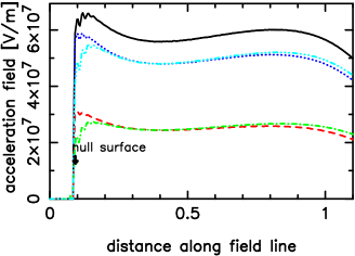
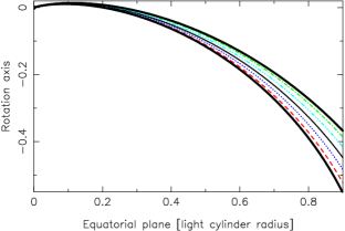
Figure 3: Left: The field-aligned electric field of a sub-GJ current solution at five discrete heights (see right panel) for $\alpha_{\rm i}=70^{\circ}$ and $h_{\rm m}=0.047$. The abscissa indicates the distance along the field line from the star in the unit of the light-cylinder radius. The null surface position at the height $h=h_{\rm m}/2$ is indicated by the down arrow. Right: Magnetic field lines on the poloidal plane in which both the rotational and magnetic axes reside. Instead of $h_{\rm m}=0.047$, $h_{\rm m}=0.200$ is adopted for clarity. The thick solid curves denote the lower and upper boundaries, while the thin dashed, dotted, solid, dash-dot-dot-dotted, and dash-dotted ones give the same $h/h_{\rm m}$ values as those in the left panel; they are $h/h_{\rm m}=2/16$, $5/16$, $8/16$, $11/16$, and $14/16$, respectively.

Examine a sub-GJ current solution, which is defined by $j_{\rm e}<|\rho_{{\rm GJ}}/(\Omega B/2\pi c)|_{s=0}\approx(1-\omega/\Omega)B_{z\ast}/B_{\ast}$, where $B_{z\ast}$ refers to the surface magnetic field component projected along the rotation axis; the right-hand side is evaluated at $s=0$ and $\theta_{\ast}=\theta_{\ast}^{\rm max}$. To this aim, we consider a transversely thin gap, $h_{\rm m}=0.047$. The solution becomes similar to the vacuum one obtained in the traditional outer-gap model model (CHR86a), as the left panel of figure 3 indicates. In this figure, we present $E_{\parallel}(s,h)$ at discrete height $h$ ranging from $2h_{\rm m}/16$, $5h_{\rm m}/16$, $8h_{\rm m}/16$, $11h_{\rm m}/16$, $14h_{\rm m}/16$, with dashed, dotted, solid, dash-dot-dot-dot, and dash-dotted curves, respectively; they are depicted in the right panel with a larger $h_{\rm m}$ ($=0.200$) for illustration purpose. For one thing, for such a transversely thin, nearly vacuum gap, the inner boundary is located slightly inside of the null surface. What is more, $E_{\parallel}$ maximizes at the central height, $h=h_{\rm m}/2$, and remains roughly constant in the entire region of the gap. The solved $E_{\parallel}$ distributes almost symmetrically with respect to the central height; for example, the dashed and dash-dotted curves nearly overlap each other. Similar solutions are obtained for a thiner gap, $h_{\rm m}<0.047$.

3.3 Super-GJ current solution: Hybrid gap structure

Next, let us consider a thicker gap, $h_{\rm m}=0.048$. In this case, $j_{\rm e}$ becomes comparable or greater than $|\rho_{{\rm GJ}}/(\Omega B/2\pi c)|_{s=0}$ in the upper half region $h>h_{\rm m}/2$ of the gap, deviating the solution from the vacuum one. In the left panel of figure 4, we present $E_{\parallel}(s,h)$ at five discrete height $h$ in the same way as figure 3. It follows that $E_{\parallel}$ is screened by the discharge of created pairs in the inner-most region ($s<0.3\varpi_{\rm LC}$) in the higher latitudes ($h>h_{\rm m}/2$). For example, $E_{\parallel}$ at $h=7h_{\rm m}/8$ (dash-dotted curve) deviates from the unscreened solution at the lower latitudes $h=h_{\rm m}/8$ (dashed). On the other hand, along the lower field lines ($h<h_{\rm m}/2$), $E_{\parallel}(s)$ is roughly constant as in the traditional outer-gap model.

Let us further consider a thicker gap, $h_{\rm m}=0.060$. The right panel of figure 4 shows that $E_{\parallel}(s,h)$ is substantially screened than the marginally super-GJ case, $h_{\rm m}=0.048$ (left panel). Because the gap transfield thickness virtually shrinks in $s<0.5\varpi_{\rm LC}$ due to screening in the higher latitudes, $E_{\parallel}$ in the lower latitudes also decreases compared to smaller $h_{\rm m}$ cases, as the dashed lines in the left and right panels indicate.

To understand the screening mechanism, it is helpful to examine the Poisson equation (22), which is a good approximation in $s<0.4\varpi_{\rm LC}$. In the transversely thin limit, it becomes

$$-\frac{1}{(1-r_{\rm g}/r)}\frac{1}{r_{\ast}^{2}}\frac{B(r)}{B_{\ast}}\frac{\partial^{2}\Psi}{\partial\theta_{\ast}^{2}}\approx 4\pi(\rho-\rho_{{\rm GJ}})\approx\frac{2\Omega B(r)}{c}\left(\frac{\rho}{\Omega B/2\pi c}-\frac{\rho_{{\rm GJ}}}{\Omega B/2\pi c}\right).$$ (67)

Since we are interested in the second-order $\theta_{\ast}$ derivatives, this equation is valid not only for a nearly aligned rotator, but also for an oblique rotator. We could directly check it from the general equation (13). Factoring out the magnetic field expansion factor, $B(r)/B_{\ast}$, from the both sides, we obtain

$$\Psi\approx\left(1-\frac{r_{\rm g}}{r}\right)\frac{\Omega B_{\ast}}{c}\left(\frac{\rho}{\Omega B/2\pi c}-\frac{\rho_{{\rm GJ}}}{\Omega B/2\pi c}\right)r_{\ast}^{2}(\theta_{\ast}-\theta_{\ast}^{\rm min})(\theta_{\ast}^{\rm max}-\theta_{\ast}).$$ (68)

We thus find that $E_{\parallel}\equiv-\partial\Psi/\partial s$ is approximately proportional to $-\partial(\rho/B-\rho_{{\rm GJ}}/B)/\partial s$. It is, therefore, important to examine the two-dimensional distribution of $\rho/B$ and $\rho_{{\rm GJ}}/B$ to understand $E_{\parallel}(s,h)$ behavior.

In figure 5, we present $\rho/(\Omega B/2\pi c)$, $\rho_{\rm e}/(\Omega B/2\pi c)$, and $\rho_{{\rm GJ}}/(\Omega B/2\pi c)$, as the solid, dash-dotted, and dashed curves, at nine discrete magnetic latitudes, ranging from $h=(4/16)h_{\rm m}$, $(5/16)h_{\rm m}$, $\ldots$, to $(12/16)h_{\rm m}$ for the same parameters as the right panel of figure 4. If there is a cold-field ion emission from the star, the total charge density (solid curve) deviates from the created charge density (dash-dotted one). It follows that the current is sub-GJ for $h\leq(5/16)h_{\rm m}=0.0187$ and super-GJ for $h\geq(6/16)h_{\rm m}=0.0225$. Along the field lines with super-GJ current, $\rho_{\rm e}-\rho_{{\rm GJ}}$ becomes negative close to the star. This inevitably leads to a positive $E_{\parallel}$, which extracts ions from the stellar surface. In this paper, we assume that the extracted ions consist of protons; nevertheless, the conclusions are little affected by the composition of the extracted ions.

In the outer region, $\rho/B$ levels off in $s>0.5\varpi_{\rm LC}$ for $h>h_{\rm m}/2$. Since $\rho_{{\rm GJ}}/B$ becomes approximately a linear function of $s$, $E_{\parallel}$ remains nearly constant in $s>0.5\varpi_{\rm LC}$, in the same manner as in traditional outer-gap model. In the inner region, on the other hand, inward-directed $\gamma$-rays propagate into the convex side due to the field line curvature, increasing particle density exponentially with $h$. As a result, the lower part (i.e., smaller $h$ region) becomes nearly vacuum. For example, at $h=h_{\rm m}/4=0.015$ (top left panel), positive $\rho_{\rm e}-\rho_{{\rm GJ}}$ leads to a negative $E_{\parallel}$ at the stellar surface, inducing no ion emission. Even though the created current is sub-GJ at $h=0.0187$, ions are extracted from the surface. This is because the negative $\rho_{\rm eff}\equiv\rho-\rho_{{\rm GJ}}$ in the higher latitudes $h\geq 0.0225$ cancels the relatively small positive $\rho_{\rm eff}$ along $h=0.0187$ to induce a positive $E_{\parallel}$ at the stellar surface. Such a two-dimensional effect in the Poisson equation is also important in the higher altitudes ($0.1\varpi_{\rm LC}<s<0.3\varpi_{\rm LC}$) along the higher-latitude field lines($h\geq 0.0225$). Outside of the null surface, $s>0.09\varpi_{\rm LC}$, there is a negative $\rho_{\rm eff}$ in the sub-GJ current region ($h\leq 0.015$). This negative $\rho_{\rm eff}$ works to prevent $E_{\parallel}$ from vanishing in the higher latitudes, where pair creation is copious. However, the created pairs discharge until $E_{\parallel}$ vanishes, resulting in a larger gradient of $\rho$ than that of $\rho_{{\rm GJ}}$ in the intermediate latitudes in $0.0225\leq h\leq 0.0262$. In the upper half region ($0.03\leq h<h_{\rm m}=0.06$), $\partial\rho/\partial s$ does not have to be greater than $\partial\rho_{{\rm GJ}}/\partial s$, in order to screen $E_{\parallel}$.

In short, the gap has a hybrid structure: The lower latitudes (with small $h$) are nearly vacuum having sub-GJ current densities and the inner boundary is located slightly inside of the null surface, because $\Psi>0$ region will be filled with the electrons emitted from the stellar surface. The higher latitudes, on the other hand, are non-vacuum having super-GJ current densities, and the inner boundary is located at the stellar surface, extracting ions at the rate such that their non-relativistic column density at the stellar surface cancels the strong $E_{\parallel}$ induced by the negative $\rho-\rho_{{\rm GJ}}$ of relativistic electrons, positrons, and ions. The created pairs discharge such that $E_{\parallel}$ virtually vanishes in the region where pair creation is copious. Thus, in the intermediate latitudes between the sub-GJ and super-GJ regions, $\partial\rho/\partial s>\rho_{{\rm GJ}}/\partial s$ holds.

Even though the inner-most region of the gap is inactive, general relativistic effect (space-time dragging effect, in this case) is important to determine the ion emission rate from the stellar surface. For example, at $h=h_{\rm m}/2$ for $h_{\rm m}=0.600$ (i.e., the central panel in fig. 5), $j_{\rm ion}$ is $69$% greater than what would be obtained in the Newtonian limit, $\rho_{{\rm GJ}}=-\mbox{\boldmath$\Omega$}\cdot\mbox{\boldmath$B$}/2\pi c$. This is because the reduced $|\rho_{{\rm GJ}}|$ near the star (about $15$% less than the Newtonian value) enhances the positive $E_{\parallel}$, which has to be canceled by a greater ion emission (compared to the Newtonian value). The current, $j_{\rm ion}$, is adjusted so that $|\rho_{\rm eff}|$ may balance with the trans-field derivative of $\Psi$ near the star. The resultant $|\rho_{\rm eff}|$ becomes small compared to $|\rho_{{\rm GJ}}|$, in the same manner as in traditional polar-cap models, which has a negative $E_{\parallel}$ with electron emission from the star. Although the non-relativistic ions have a large positive charge density very close to the star (within $10$ cm from the surface), it cannot be resolved in figure 5. Note that the present calculation is performed from the stellar surface to the outer magnetosphere and does not contain a region with $E_{\parallel}<0$. It follows that an accelerator having $E_{\parallel}<0$ (e.g., a polar-cap or a polar-slot-gap accelerator) cannot exist along the magnetic field lines that have an super-GJ current density created by the mechanism described in the present paper.

It is worth examining how $E_{\parallel}$ changes with varying $h_{\rm m}$. In figure 6, we present $E_{\parallel}(s,h)$ at the central height $h=h_{\rm m}/2$. In the left panel, the dotted, solid, dashed, and dash-dotted curves correspond to $h_{\rm m}=0.047$, $0.048$, $0.060$, and $0.100$, respectively, while in the right panel, the dash-dotted, dash-dot-dot-dotted, solid, and dashed ones to $0.100$, $0.160$, $0.200$, and $0.240$, respectively. It follows that the inner part of the gap becomes substantially screened by the discharge of created pairs as $h_{\rm m}$ increases. It also follows that the maximum of $E_{\parallel}$ increases with increasing $h_{\rm m}$ for $h_{\rm m}<0.2$, because the two-dimensional screening effect due to the zero-potential walls becomes less important for a larger $h_{\rm m}$. To solve particle and $\gamma$-ray Boltzmann equations, we artificially put $E_{\parallel}=0$ in $\varpi>0.9\varpi_{\rm LC}$, or equivalently in $s>1.1\varpi_{\rm LC}$ for $\alpha_{\rm i}=70^{\circ}$, as mentioned in § 2.5.

The created current density, $j_{\rm e}$, is presented in figure 7, as a function of $h$. The thin dashed line represents $|\rho_{{\rm GJ}}/(\Omega B/2\pi c)|_{s=0}$; if $j_{\rm e}$ appears below (or above) this line, the created current is sub- (or super-) GJ along the field line specified by $h$. The open and filled circles denote the lowest and highest latitudes that are used in the computation. For $h_{\rm m}=0.047$, the solution (dotted curve) is sub-GJ along all the field lines; thus, screening due to the discharge is negligible as the dotted curve in the left panel of figure 6 shows. As $h_{\rm m}$ increases, the solution becomes super-GJ from the higher latitudes, as indicated by the solid ($h_{\rm m}=0.048$), dashed ($h_{\rm m}=0.060$), dash-dotted ($h_{\rm m}=0.100$), and dash-dot-dot-dotted ($h_{\rm m}=0.160$) curves in figure 7. As a result, screening becomes significant as $h_{\rm m}$ increase, as figure 6 shows. This screening of $E_{\parallel}$ has a negative feed back effect in the sense that $j_{\rm e}$ is regulated below unity. Even though it is not resolved in figure 6, in the lower latitudes, $j_{\rm e}$ grows across the gap height exponentially, as CHR86a suggested. For example, $j_{\rm e}=3.0\times 10^{-10}$, $2.1\times 10^{-9}$, $2.1\times 10^{-8}$, $1.0\times 10^{-7}$, $4.3\times 10^{-7}$, $1.0\times 10^{-6}$, $4.6\times 10^{-5}$, and $1.3\times 10^{-1}$ at $h/h_{\rm m}=1/16$, $2/16$, $3/16$, $\ldots$, $8/16$, respectively, for $h_{\rm m}=0.048$ (solid curve). This is because the pair creation rate at height $h$ is proportional to the number of $\gamma$-rays that are emitted by charges on all field lines below $h$.

Let us now turn to the emitted $\gamma$-rays. Figure 8 shows the phase-averaged $\gamma$-ray spectrum calculated for three different $h_{\rm m}$’s. Open circles denote the pulsed fluxes detected by COMPTEL (below 30 MeV; Ulmer et al. 1995, Kuiper et al. 2001) and EGRET (above 30 MeV; Nolan et al. 1993, Fierro et al. 1998), while the open square does the upper limit obtained by CELESTE (de Naurois et al. 2002). It follows that the sub-GJ (i.e., traditional outer-gap) solution with $h_{\rm m}=0.047$ predicts too small $\gamma$-ray flux compared with the observations. (Note that in traditional outer-gap models, particle number density is assumed to be the Goldreich-Julian value, while $E_{\parallel}$ is given by the vacuum solution of the Poisson equation, which is inconsistent.) The maximum flux, which appears around GeV energies, does not become greater than $10^{11}$ Jy Hz for any sub-GJ solutions, whatever values of $\alpha_{\rm i}$, $\mu$, and $kT_{\rm s}$ we may choose. Thus, we can rule out the possibility of a sub-GJ solution for the Crab pulsar.

As $h_{\rm m}$ increases, the increased $E_{\parallel}$ results in a harder curvature spectrum, as the solutions corresponding to $h_{\rm m}=0.100$ and $0.200$ indicate. As will be discussed in § 4.1, the problem of insufficient $\gamma$-ray fluxes may be solved if we consider a three-dimensional gap structure. However, the secondary synchrotron flux emitted outside of the gap is too small to explain the flat spectral shape below 100 MeV. The $\gamma$-ray spectrum is nearly unchanged for $0.2\leq h_{\rm m}\leq 0.3$. For $h_{\rm m}>0.3$, the $\gamma$-ray flux tends to decrease, because the $E_{\parallel}(s)$ peaks outside of the artificial outer boundary, $r\sin\theta=0.9\varpi_{\rm LC}$, which corresponds to $s=1.1\varpi_{\rm LC}$ for $\alpha_{\rm i}=70^{\circ}$. For $h_{\rm m}>0.4$, the gap virtually vanishes because of the discharge of copiously created pairs; in another word, the gap is located outside of $r\sin\theta=0.9\varpi_{\rm LC}$. On these grounds, we cannot reproduce the observed flat spectral shape if we consider $kT_{\rm s}=100$ eV, $\mu=4.0\times 10^{30}\mbox{ G cm}^{3}$, and $\alpha_{\rm i}=70^{\circ}$, no matter what value of $h_{\rm m}$ is adopted. Therefore, in the next three subsections, we examine how the solution changes if we adopt different values of $kT_{\rm s}$, $\mu$, and $\alpha_{\rm i}$.

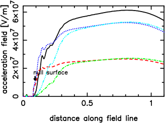
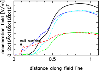
Figure 4: Same figure as figure 3: $E_{\parallel}(s,h)$ of two super-GJ current solutions for $h_{\rm m}=0.048$ (left) and $0.060$ (right) at five discrete $h$’s.

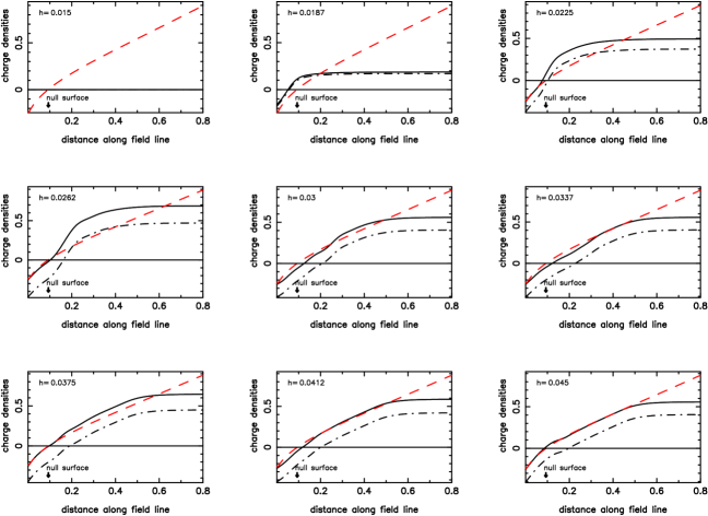
Figure 5: Total (solid), created (dash-dotted), and Goldreich-Julian (dashed) charge densities in $\Omega B(s,h)/(2\pi c)$ unit, for $\alpha_{\rm i}=70^{\circ}$ and $h_{\rm m}=0.060$ at nine transfield heights, $h$. If there is an ion emission from the stellar surface, the total charge density deviates from the created one.

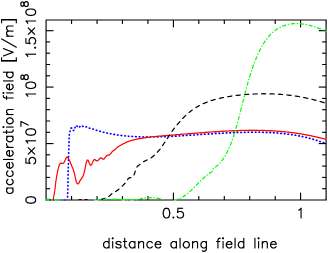
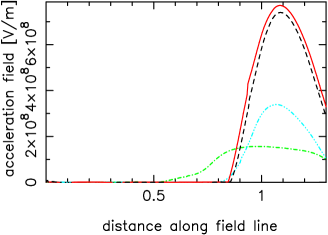
Figure 6: Field-aligned electric field at $h=h_{\rm m}/2$ as a function of $s/\varpi_{\rm LC}$ for $\mu=4.0\times 10^{30}\mbox{ G cm}^{3}$, $kT_{\rm s}=100$ eV, and $\alpha_{\rm i}=70^{\circ}$. Left: The dotted, solid, dashed, and dash-dotted curves corresponds to $h=0.047$, $0.048$, $0.060$, and $0.100$; right: The dash-dotted, dash-dot-dot-dotted, solid, and dashed curves corresponds to $h=0.100$, $0.160$, $0.200$, and $0.240$.

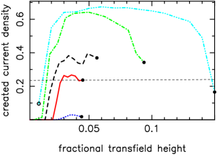
Figure 7: Created current density $j_{\rm e}$ (in unit of $\Omega B/2\pi$) as a function of the transfield thickness $h$ for $\mu=4.0\times 10^{30}\mbox{ G cm}^{3}$, $kT_{\rm s}=100$ eV, and $\alpha_{\rm i}=70^{\circ}$. The dotted, solid, dashed, dash-dotted, and dash-dot-dot-dotted curves corresponds to $h=0.047$, $0.048$, $0.060$, $0.100$, and $0.160$, respectively.

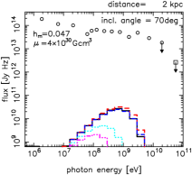
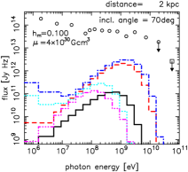
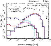
Figure 8: Calculated phase-averaged spectra of the pulsed, outward-directed $\gamma$-rays for $\alpha_{\rm i}=70^{\circ}$, $kT_{\rm s}=100$ eV, and $\mu=4.0\times 10^{30}\mbox{ G cm}^{3}$, with three different gap thickness, $h_{\rm m}$. The flux is averaged over the meridional emission angles between $44^{\circ}$ and $58^{\circ}$ (solid), $58^{\circ}$ and $72^{\circ}$ (dashed), $72^{\circ}$ and $86^{\circ}$ (dash-dotted), $86^{\circ}$ and $100^{\circ}$ (dotted), $100^{\circ}$ and $114^{\circ}$ (dash-dot-dot-dotted), from the magnetic axis on the plane in which both the rotational and magnetic axes reside.

3.4 Dependence on Surface Temperature

In the same manner as in § 3.3, we calculate $E_{\parallel}(s,h=h_{\rm m}/2)$ for $kT_{\rm s}=150$ eV to find that their distribution is similar to $kT_{\rm s}=100$ eV case (i.e., fig. 6). For example, sub/super-GJ current solutions are discriminated by the condition whether $h_{\rm m}$ is greater than $0.048$ or not, and the maximum of $E_{\parallel}$ is $7.2\times 10^{8}\mbox{ V m}^{-1}$ for $0.20<h_{\rm m}<0.24$. Other quantities such as the particle and $\gamma$-ray distribution functions are also similar. Therefore, we can conclude that the solution is little subject to change for the variation of $kT_{\rm s}$, even though the photon-photon pair production rate increases with increasing $kT_{\rm s}$. This is due to the negative feedback effect, which will be discussed in § 4.2.

3.5 Dependence on Magnetic Moment

Let us examine how the solution depends on the magnetic moment, $\mu$. In figure 9, we present $E_{\parallel}(s,h=h_{\rm m}/2)$ for seven discrete $h_{\rm m}$’s with $\mu=6.0\times 10^{30}\mbox{ G cm}^{3}$; in the left panel, the dotted and solid curves correspond to $h=0.039$ and $0.041$, respectively, instead of $h=0.047$ and $0.048$ in figure 6. It follows that the exerted $E_{\parallel}$ is greater than the case of $\mu=4.0\times 10^{30}\mbox{ G cm}^{3}$ (fig. 6), because $\rho_{{\rm GJ}}$ increases $1.5$ times. The negative feedback effect cannot cancel the increase of $\mu$, unlike the increase of $kT_{\rm s}$, because the right-hand side of equation (19) is more directly affected by the variation of $\mu$ through $\rho_{{\rm GJ}}$ than by the variation of $kT_{\rm s}$ through pair creation.

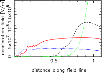
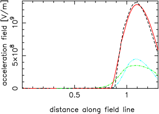
Figure 9: Same figure as figure 6 but with $\mu=6.0\times 10^{30}\mbox{ G cm}^{3}$; in the left panel, the dotted and solid curves correspond to $h=0.039$ and $0.041$, respectively. For other two curves in the left panel and four curves in the right panel, $h$ takes the same values as in figure 6.

We also present the $\gamma$-ray spectrum for three different $\mu$’s in figure 10. It follows that both the peak energy and the flux of curvature $\gamma$-rays (around GeV energies) increase with increasing $\mu$. This is because $\rho_{{\rm GJ}}$, and hence $E_{\parallel}$ increases with $\mu$. It also follows that the secondary synchrotron flux (below 100 MeV) increases with $\mu$, because the magnetic field strength increases in the magnetosphere. We find that a larger magnetic dipole moment, $\mu\geq 6\times 10^{30}\mbox{\,G\,cm}^{3}$ is preferable to explain the observed pulsed flux from the Crab pulsar.

If we adopt $\mu=8\times 10^{30}\mbox{\,G\,cm}^{3}$, which is about twice larger than the dipole deduced value, the spectral shape becomes more consistent compared with smaller $\mu$ cases. We should notice here that the moment of inertia, $I$, have to be large in this case. For example, if we assume a pure magnetic dipole radiation, the spin-down luminosity becomes $L_{\rm SD}=(2\sin^{2}\alpha_{\rm i}/3)(\mu^{2}\Omega^{4}/c^{3})=1.7\times 10^{39}\mbox{\,ergs\ s}^{-1}$ for $\alpha_{\rm i}=70^{\circ}$. Equating $-\dot{E}=-I\Omega\dot{\Omega}$ with this $L_{\rm SD}$, we obtain $I=3.9\times 10^{45}\mbox{\,g\ cm}^{2}$, which is consistent with the limit ($I>3.04\times 10^{45}\mbox{\,g\ cm}^{2}$) derived from the consideration of energetics of the Crab nebula (Bejger & Haensel 2002). However, solving the time-dependent equations of force-free electrodynamics, Spitkovsky (2006) derived $L_{\rm SD}\approx(1+\sin^{2}\alpha_{\rm i})(\mu^{2}\Omega^{4}/c^{3})$, which gives $\approx 5.6\times 10^{39}\mbox{\,ergs\ s}^{-1}$ for $\alpha_{\rm i}=70^{\circ}$. This large spin-down luminosity results in $I\approx 1.2\times 10^{46}\mbox{\,g\ cm}^{2}$, which is too large even compared with those obtained for stiff equation of state (Serot 1979a, b; Pandharipande & Smith 1975). Thus, it implies either that $\mu$ should be less than $8\times 10^{30}\mbox{\,G\,cm}^{3}$ or that the deduced magnetospheric current is too large when the relationship $L_{\rm SD}\approx(1+\sin^{2}\alpha_{\rm i})(\mu^{2}\Omega^{4}/c^{3})$ is derived (for a discussion of the magnetospheric current determination, see section 4 of Hirotani 2006).

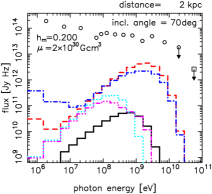
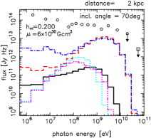
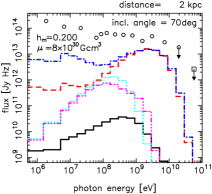
Figure 10: Same figure as figure 8 for $\alpha_{\rm i}=70^{\circ}$, $kT_{\rm s}=100$ eV, and $h_{\rm m}=0.200$, with different dipole moment, $\mu$.

3.6 Dependence on Magnetic Inclination

Let us examine how the solution depends on the magnetic inclination angle, $\alpha_{\rm i}$. Figure 11 shows the $\gamma$-ray spectra for $\mu=6\times 10^{30}\mbox{ G cm}^{3}$, $kT_{\rm s}=100$ eV, $h_{\rm m}=0.200$, with three different inclination, $\alpha_{\rm i}=50^{\circ}$, $60^{\circ}$, and $80^{\circ}$, in the same manner as in figure 8. The flux is averaged over the meridional emission angles between $44^{\circ}$ and $58^{\circ}$ (solid), $58^{\circ}$ and $72^{\circ}$ (dashed), $72^{\circ}$ and $86^{\circ}$ (dash-dotted), $86^{\circ}$ and $100^{\circ}$ (dotted), $100^{\circ}$ and $114^{\circ}$ (dash-dot-dot-dotted), from the magnetic axis on the plane in which both the rotational and magnetic axes reside. We find that the $\gamma$-ray flux reaches a peak of $\sim 2\times 10^{13}$ Jy Hz around 2 GeV and that this peak does not strongly depend on $\alpha_{\rm i}$. This is because the pair creation efficiency, which governs the gap electrodynamics, crucially depends on the distance from the star, which has a small dependence on $\alpha_{\rm i}$. However, we also find that the flux tends to be emitted into larger meridional angles from the magnetic axis (i.e., from outer regions) for smaller $\alpha_{\rm i}$. The reasons are fourfold:
(1) $\rho_{{\rm GJ}}$ decreases with decreasing $\alpha_{\rm i}$ at a fixed $s$; as a result, the null surface appears at larger $s$ for smaller $\alpha_{\rm i}$.
(2) $\rho_{{\rm GJ}}(s)=-\rho_{{\rm GJ}}(0)$ is realized at larger $s$ for smaller $\alpha_{\rm i}$.
(3) In the region where $\rho_{{\rm GJ}}<-\rho_{{\rm GJ}}(0)$ holds, $E_{\parallel}$ is substantially screened by the discharge of created pairs. (Compare fig. 5 and the right panel of fig. 4.)
(4) The unscreened $E_{\parallel}$ tends to appear at larger $s$ for smaller $\alpha_{\rm i}$, resulting in a $\gamma$-ray emission which concentrate in larger meridional angles.
We can alternatively interpret the explanation above as follows:
(a) $|\rho_{{\rm GJ}}(0)|$ increases with decreasing $\alpha_{\rm i}$.
(b) The created current density, $j_{\rm e}$, which is greater than $c|\rho_{{\rm GJ}}(0)|$ for a super-GJ solution, increases with decreasing $\alpha_{\rm i}$. For example, we obtain $j_{\rm e}=0.62$, $0.67$, $0.74$, and $0.77$ for $\alpha_{\rm i}=80^{\circ}$, $70^{\circ}$, $60^{\circ}$, and $50^{\circ}$, respectively, at $h=h_{\rm m}/2=0.100$ with $\mu=6\times 10^{30}\mbox{ G cm}^{3}$, and $kT_{\rm s}=100$ eV.
(c) A larger $j_{\rm e}$ results in a larger injection of the discharged positrons and the emitted ions into the strong-$E_{\parallel}$ region from the stellar side.
(d) A larger injection of positive charges from the stellar side shifts the gap outwards by the mechanism discussed in § 2 of Hirotani and Shibata (2001a).

For a smaller inclination, $\alpha_{\rm i}\leq 40^{\circ}$, the gap is located in $\varpi>0.9\varpi_{\rm LC}$; that is, no super-GJ solution exists. Therefore, the observed $\gamma$-ray flux cannot be explained by the present theory, if the magnetic inclination is constrained to be less than $40^{\circ}$ by some other methods.

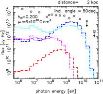
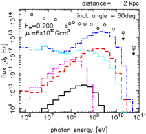
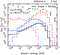
Figure 11: Same figure as figure 8 for $kT_{\rm s}=100$ eV, $\mu=6.0\times 10^{30}\mbox{ G cm}^{3}$, and $h_{\rm m}=0.200$ with different magnetic inclination angle, $\alpha_{\rm i}$.

3.7 Particle Distribution Functions

Let us examine how the particle distribution function evolves at different positions. Figure 12 represents the evolution of positronic distribution function from $s=0.85\varpi_{\rm LC}$ (dashed curve), $0.90\varpi_{\rm LC}$ (dash-dotted), $0.95\varpi_{\rm LC}$ (dash-dot-dot-dotted), $1.00\varpi_{\rm LC}$ (solid), to $1.30\varpi_{\rm LC}$ (dotted). It shows that the positrons are injected into the strong-$E_{\parallel}$ region ($s>0.85\varpi_{\rm LC}$) with energies $10^{4}<\Gamma<3\times 10^{6}$ because of the acceleration by the small-amplitude, residual $E_{\parallel}$ in $s<0.85\varpi_{\rm LC}$ (solid curve in the right panel of fig. 9). The positrons are accelerated outwards to attain $\Gamma\sim 4\times 10^{7}$ at $s\sim 1.0\varpi_{\rm LC}$. They are subsequently decelerated by curvature cooling in $\varpi>0.9\varpi_{\rm LC}$ (or equivalently $s>1.1\varpi_{\rm LC}$ for $\alpha_{\rm i}=70^{\circ}$), where we artificially put $E_{\parallel}=0$, to escape outwards with $\Gamma\sim 10^{7}$ at $s\sim 1.3\varpi_{\rm LC}$. There is a small population of the positrons that have upscattered surface X-rays to possess smaller energies than the curvature-limited positrons. For example, within the gap ($s<1.1\varpi_{\rm LC}$), the dash-dotted, dash-dot-dot-dotted, and solid curves have the broad, lower-energy component, which connects with the curvature-limited peak component. However, in $s>1.1\varpi_{\rm LC}$, we artificially put $E_{\parallel}=0$; as a result, the positrons that have lost energies by ICS cannot be re-accelerated, forming a separate component in $\Gamma<4\times 10^{6}$ from the curvature-limited peak component, as the dotted curve shows. The upscattered photons obtain several TeV energies; however, they are totally absorbed by the strong magnetospheric infrared radiation field. Therefore, we depict only the photon energies below $100$ GeV in figures 8, 10, and 11.

Since most of the pairs are created inwards, positrons return to migrate outwards by the small-amplitude $E_{\parallel}$ in $s<0.85\varpi_{\rm LC}$ (for $\mu=6.0\times 10^{30}\mbox{ G cm}^{3}$ and $\alpha_{\rm i}=70^{\circ}$), losing significant transverse momenta via synchrotron process to fall onto the ground-state Landau level in strong $B$ region. Thus, their emission in strong-$E_{\parallel}$ region is given by a pure-curvature formula.

Next, we consider the distribution function of electrons. In figure 13 we present their evolution along the field line $h=h_{\rm m}/2=0.100$ from $s=0.90\varpi_{\rm LC}$ (dash-dot-dot-dotted curve), $0.40\varpi_{\rm LC}$ (dotted), $0.20\varpi_{\rm LC}$ (dash-dotted), $0.08\varpi_{\rm LC}$ (dashed), to $0$ (solid). Left panel shows the energy spectrum. Electrons created in $s<0.85\varpi_{\rm LC}$ cannot be accelerated by $E_{\parallel}$ efficiently; thus, their energy spectrum becomes broad as the dotted, dashed-dotted, and dashed curves indicate (i.e., particle Lorentz factors do not concentrate at the curvature-limited terminal value). From $s=0.08\varpi_{\rm LC}$ to $s=0$, electrons are decelerated via synchro-curvature radiation and non-resonant inverse-Compton scatterings. Finally, they hit the stellar surface with $\Gamma<3\times 10^{5}$. Assuming that the azimuthal gap width is $\pi$ radian, we obtain $L_{\rm PC}=2.6\times 10^{31}\mbox{\,ergs s}^{-1}$ as the heated polar-cap luminosity. Thus, the X-ray emission due to the bombardment is negligible, compared with the total soft-X-ray luminosity (0.1–2.4 keV) of $7.6\times 10^{34}\mbox{\,ergs s}^{-1}(\Delta\Omega_{\rm X}/\mbox{ster})$ (e.g., Becker & Trümper 1997), where $\Delta\Omega_{\rm X}$ refers to the emission solid angle.

Let us see the pitch angle evolution of the electrons, which is presented by the right panel of figure 13. In the outer part of the gap, the electrons are created by the collisions between the outward-directed $\gamma$-rays and the surface X-rays. Thus, created electrons have outward momenta initially, then return by the positive $E_{\parallel}$, losing their perpendicular momentum substantially via synchrotron radiation. Thus, at $s=0.90\varpi_{\rm LC}$, the dash-dot-dot-dotted curve show that their pitch angles, $\chi$, are less than $8\times 10^{-5}$. However, most of the pairs are created by the inward-directed $\gamma$-rays in $s<0.6\varpi_{\rm LC}$; thus, electrons have initial inward momenta to migrate inwards by the small-amplitude, residual $E_{\parallel}$. Since such inward-created electrons do not change their migration direction, their pitch angles are greater than those of the outward-created ones, as the dotted curve demonstrates. As the electrons migrate inwards, they lose perpendicular momenta via synchro-curvature radiation in the strong $B$ field, reducing their pitch angles, as the dotted, dash-dotted, and dashed curves indicate.

We should point out that a pure curvature formula cannot be applied to the electrons. For example, at $s=0.4\varpi_{\rm LC}$, the dotted curve in figure 13 demonstrates that electrons have $10^{4}<\Gamma<10^{7}$ and $10^{-8}<\sin\chi<10^{-3.5}$. Noting that we have $B=3.0\times 10^{7}$ G at $s=0.4\varpi_{\rm LC}$, we find that newly created electrons, which have lower-energies ($\Gamma<10^{6}$) and larger pitch angles ($\sin\chi>10^{-5}$), emit synchro-curvature radiation, rather than pure-curvature one, as figure 14 shows. At $s=0.2\varpi_{\rm LC}$, we have $B=3.6\times 10^{8}$ G; thus, the dash-dotted curve shows that the pure-curvature formula is totally inapplicable as we consider a smaller distance from the star. The only exception is the inner-most region ($s<5r_{\ast}=0.031\varpi_{\rm LC}$ and $B>5\times 10^{10}$ G), where electrons suffer substantial de-excitation via synchrotron radiation, falling at last onto the ground-state Landau level. In this region, electrons emit via pure curvature radiation. We thus artificially assume $\sin\chi=10^{-20}$, which guarantees pure curvature emission, and do not depict the solid curve in the right panel of figure 13. Since pair creation and the resultant screening of $E_{\parallel}$ is governed by the inward-directed $\gamma$-ray flux and spectrum, it is essential to adopt the correct radiation formula by computing the pitch-angle evolution of inward-migrating particles.

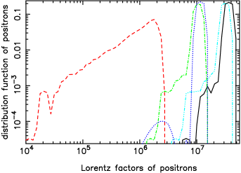
Figure 12: Energy spectrum of positrons at $s=0.85\varpi_{\rm LC}$ (dashed), $0.90\varpi_{\rm LC}$ (dash-dotted), $0.95\varpi_{\rm LC}$ (dash-dot-dot-dotted), $1.00\varpi_{\rm LC}$ (solid), and $1.30\varpi_{\rm LC}$ (dotted), for $\alpha_{\rm i}=70^{\circ}$, $\mu=6.0\times 10^{30}\mbox{ G cm}^{3}$, $kT_{\rm s}=100$ eV, and $h_{\rm m}=0.20$.

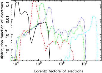
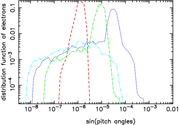
Figure 13: Distribution function of electrons at $s=0.9\varpi_{\rm LC}$ (dash-dot-dot-dotted), $0.4\varpi_{\rm LC}$ (dotted), $0.2\varpi_{\rm LC}$ (dash-dotted), $0.08\varpi_{\rm LC}$ (dashed), and $0$ (solid), for $\alpha_{\rm i}=70^{\circ}$, $\mu=6.0\times 10^{30}\mbox{ G cm}^{3}$, $kT_{\rm s}=100$ eV, and $h_{\rm m}=0.20$. Left panel shows the Lorentz factor dependence, while the right one shows the pitch angle dependence.

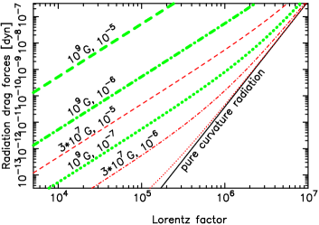
Figure 14: Pure-curvature (solid) vs. synchro-curvature radiation-reaction forces. For the latter, we adopt the pitch angles $\chi=10^{-5}$, $10^{-6}$, and $10^{-7}$ rad for the dashed, dash-dotted, and dotted curves, respectively, and $B=3\times 10^{7}$ and $10^{9}$ G for the thin and thick ones, respectively. Curvature radius is assumed to be $0.4\varpi_{\rm LC}=6.37\times 10^{7}$ cm.

3.8 Formation of Magnetically Dominated Wind

Let us finally consider the magnetic dominance within the light cylinder. First, introduce the magnetization parameter,

$$\sigma \equiv \frac{B^{2}}{4\pi}\left\{\Gamma m_{\rm e}c^{2}\int\!\!\!\!\!\int\!\!\!\!\!\int(N_{+}+N_{-})d^{3}\mbox{\boldmath$p$}+\Gamma_{\rm ion}m_{\rm ion}c^{2}\int\!\!\!\!\!\int\!\!\!\!\!\int N_{\rm ion}d^{3}\mbox{\boldmath$p$}\right\}^{-1}$$ (69)

$$= \frac{e(B/2)\varpi_{\rm LC}}{j_{\rm e}\Gamma m_{\rm e}c^{2}+j_{\rm ion}\Gamma_{\rm ion}m_{\rm ion}c^{2}},$$

where $N_{\rm ion}$, $\Gamma_{\rm ion}$, refers to the distribution function and the averaged Lorentz factor of the ions. Evaluating equation (69) at the light cylinder, and noting $\Gamma_{\rm ion}m_{\rm ion}c^{2}=|e\Delta\Psi_{\rm gap}|$, where $|e\Delta\Psi_{\rm gap}|\approx(B/4)h_{\rm m}^{2}\varpi_{\rm LC}$ refers to the potential drop in the gap (see eq. [68]), we obtain

$$\sigma_{\rm L}\approx\frac{1}{h_{\rm m}^{2}}\cdot\frac{2}{j_{\rm e}\Gamma m_{\rm e}c^{2}/|e\Delta\Psi_{\rm gap}|+j_{\rm ion}}.$$ (70)

Recalling $j_{\rm ion}<j_{\rm e}<1$, $\Gamma m_{\rm e}c^{2}<|e\Delta\Psi_{\rm gap}|$, and $h_{\rm m}<1$, we can conclude that the magnetic energy flux is always greater than the particle kinetic energy flux at the light cylinder, regardless of the species of the accelerated particles, of the sign of $E_{\parallel}$, or of the gap position (i.e., whether inner or outer magnetosphere). Only when the gap is formed along most of the open field lines (i.e., $h_{\rm m}\sim 1$), $\sigma_{\rm L}$ can be of the order of unity. Since the second factor in equation (70) does not change significantly for different values of parameters except for $h_{\rm m}$, $\sigma_{\rm L}$ solely depends on $h_{\rm m}$. Substituting $j_{\rm ion}\sim 0.3$, $j_{\rm e}\sim 0.6$, $\Gamma m_{\rm e}c^{2}/|e\Delta\Psi_{\rm gap}|\sim 0.25$ in $(3/16)h_{\rm m}\leq h\leq(13/16)h_{\rm m}$ for $\alpha_{\rm i}=70^{\circ}$, $\mu=6\times 10^{30}\mbox{ G cm}^{3}$, and $h_{\rm m}=0.20$, we obtain $\sigma_{\rm L}\sim 110$.

In short, along the open field lines threading the gap, Poynting flux dominates particle kinetic energy flux by a factor of 100 at the light cylinder. Positrons escape from the gap with $\Gamma\sim 10^{7}$, while ions with $\Gamma_{\rm ion}\sim 10^{4}$.

4 Summary and Discussion

To conclude, we investigated the self-consistent electrodynamic structure of a particle accelerator in the Crab pulsar magnetosphere on the two-dimensional surface that contains the magnetic field lines threading the stellar surface on the plane in which both the rotation and magnetic axes reside. We regard the trans-field thickness, $h_{\rm m}$, of the gap as a free parameter, instead of trying to constrain it. For a small $h_{\rm m}$, the created current density, $j_{\rm e}$, becomes sub-Goldreich-Julian, giving the traditional outer-gap solution but with negligible $\gamma$-ray flux. However, as $h_{\rm m}$ increases, $j_{\rm e}$ increases to become super-GJ, giving a new gap solution with substantially screened acceleration electric field, $E_{\parallel}$, in the inner part. In this case, the gap extends towards the neutron star with a small-amplitude positive $E_{\parallel}$, which extracts ions from the stellar surface. It is essential to examine the pitch-angle evolution of the created particles, because the inward-migrating particles emit $\gamma$-rays, which governs the gap electrodynamics through pair creation, via synchro-curvature process rather than pure-curvature one. The resultant spectral shape of the outward-directed $\gamma$-rays is consistent with the existing observations; however, their predicted fluxes appear insufficient. The pulsar wind at the light cylinder is magnetically dominated: Along the field lines threading the gap, magnetization parameter, $\sigma_{\rm L}$, is about $10^{2}$.

4.1 How to obtain sufficient gamma-ray flux

The obtained $\gamma$-ray fluxes in the present work, are all below the observed values. Nevertheless, this problem may be solved if we extend the current analysis into a three-dimensional configuration space. As mentioned in § 2.4, we assume $k_{\varphi}=0$ and neglect the aberration of photon emission directions. However, in a realistic three-dimensional pulsar magnetosphere, $\gamma$-rays will have angular momenta and may be emitted in a limited solid angle as suggested by the caustic model (e.g., Dyks & Rudak 2003; Dyks, Harding, & Rudak 2004), which incorporate the effect of aberration of photons and that of time-of-flight delays. In particular, in the trailing peak of a highly inclined rotator, photons emitted at different altitudes $s$ will be beamed in a narrow solid angle to be piled up at the same phase of a pulse (Morini 1983; Romani & Yadigaroglu 1995), resulting in a $\gamma$-ray flux which is an order of magnitude greater than the present values. Thus, the insufficient $\gamma$-ray fluxes does not suggest the inapplicability of the present method. It is noteworthy that the meridional propagation angles of the emitted photons (e.g., different curves in figs. 8, 10, and 11) can be readily translated into the emissivity distribution in the gap as a function of $s$. Therefore, in this work, we do not sum up the $\gamma$-ray fluxes emitted into different meridional angles taking account of the aberration of light.

4.2 Stability of the Gap

Let us discuss the electrodynamic stability of the gap, by considering whether an initial perturbation of some quantity tends to be canceled or not. In the present paper, we consider that the soft photon field is given and unchanged when gap quantities vary. Thus, let us first consider the case when the soft photon field is fixed. Imagine that the created pairs are decreased as an initial perturbation. It leads to an increase of the potential drop due to less efficient screening by the discharged pairs, and hence to an increase of particle energies. Then the particles emit synchro-curvature radiation efficiently, resulting in an increase of the created pairs, which tends to cancel the initial decrease of created pairs.

Let us next consider the case when the soft photon field also changes. Imagine again that the created pairs are decreased as an initial perturbation. It leads to an increase of particle energies in the same manner as discussed just above. The increased particle energies increase not only the number and density of synchro-curvature $\gamma$-rays, but also the surface blackbody emission from heated polar caps and the secondary magnetospheric X-rays. Even though neither the heated polar-cap emission nor the magnetospheric emission are taken into account as the soft photon field illuminating the gap in this paper, they all work, in general, to increase the pair creation within the gap, which cancels the initial decrease of created pairs more strongly than the case of the fixed soft photon field.

Because of such negative feedback effects, solution exists in a wide parameter space. For example, the created current density is almost unchanged for a wide range of $h_{\rm m}$ (e.g., compare the dash-dotted and dash-dot-dot-dotted curves in fig. 7). On these grounds, although the perturbation equations are not solved under appropriate boundary conditions for the perturbed quantities, we conjecture that the particle accelerator is electrodynamically stable, irrespective whether the X-ray field illuminating the gap is thermal or non-thermal origin.

4.3 Local vs. global currents

Let us briefly look at the relationship between the locally determined current density $j_{\rm gap}$ (eq. [43]) and the globally required one, $j_{\rm global}$. It is possible that $j_{\rm global}$ is constrained independently from the gap electrodynamics by the dissipation at large distances (Shibata 1997), which provides the electric load in the current circuit, or by the condition that the magnetic flux function should be continuous across the light cylinder, as discussed in recent force-free argument of the trans-field equation (Contopoulos, Kazanas, Fendt 1999; Goodwin et al. 2004; Gruzinov 2005; Spitkovsky 2006). In either case, $j_{\rm global}$ will be more or less close to unity (i.e., typical GJ value). On the other hand, as demonstrated in § 3.3, for super-GJ cases, $j_{\rm gap}$ is automatically regulated around $0.9$ for a wide parameter range. Thus, the discrepancy between $j_{\rm gap}$ and $j_{\rm global}$ is small provided that $h_{\rm m}$ is large enough to maintain the created current density at a super-GJ value. The small imbalance $j_{\rm global}-j_{\rm gap}$ may have to be compensated by a current injection across the outer boundary (if the gap terminates inside of the light cylinder, charged particles could be injected from the outer boundary), or by an additional ionic emission from the stellar surface (if the imbalance leads to an additional residual $E_{\parallel}$ at the surface). In any case, the injected current is small compared with $j_{\rm gap}$; thus, it will not change the electrodynamics significantly, even though the gap active region may be shifted to some degree along the magnetic field lines, as demonstrated by Hirotani and Shibata (2001a, b; 2002), TSH04, and TSHC06.

4.4 Created pairs in the inner magnetosphere

Let us devote a little more space to examining the particle flux along the open field lines that do not thread the gap (i.e., $h_{\rm m}<h<1$). Since $E_{\parallel}$ vanishes, the created, secondary pairs emit synchrotron photons, which are capable of cascading into tertiary and higher-generation pairs by $\gamma$-$\gamma$ or $\gamma$-B collisions. Examining the cascade, we can calculate the rate of pair creation, which takes place mainly in the inner magnetosphere. Denoting that the pair creation rate is $\kappa_{\rm w}(h)\cdot(\Omega B/2\pi e)$ per unit area per second, we find $\kappa_{\rm w}=2.2\times 10^{4}$, $2.1\times 10^{4}$, $1.9\times 10^{4}$, $1.8\times 10^{4}$, $1.6\times 10^{4}$, $1.1\times 10^{4}$, $1.0\times 10^{4}$, $0.99\times 10^{4}$, $0.95\times 10^{4}$, $0.96\times 10^{4}$, $1.0\times 10^{4}$ at $h=0.20125$, $0.2025$, $0.20375$, $0.205$, $0.305$, $0.405$, $0.505$, $0.605$, $0.705$, $0.805$, and $0.905$, respectively, for $\alpha_{\rm i}=70^{\circ}$, $\mu=6.0\times 10^{30}\mbox{ G cm}^{3}$, and $h_{\rm m}=0.200$. Thus, the averaged creation rate becomes ${\bar{\kappa}}_{\rm w}=1.4\times 10^{4}(\Omega B/2\pi e)$ pairs per unit area per second, giving $\dot{N}_{\rm pair}=3.8\times 10^{38}\mbox{s}^{-1}$ as the pair creation rate in the entire magnetosphere. It should be noted that this $\dot{N}_{\rm pair}$ appears less than the constraints that arise from consideration of magnetic dissipation in the wind zone (Kirk & Lyubarsky 2001, who derived $10^{40}\,\mbox{s}^{-1}$), and of Crab Nebula’s radio synchrotron emission (Arons 2004, who derived $10^{40.5}\,\mbox{s}^{-1}$).

Due to strong synchrotron radiation, these inwardly created particles quickly lose energy to fall onto the lowest Landau level, preserving longitudinal momentum $\sim m_{\rm e}c$ per particle. These non-relativistic particles possess momentum flux of $2\dot{N}_{\rm pair}m_{\rm e}c/(\pi R_{\rm PC}^{2})\sim 1.0\times 10^{12}\mbox{dyn cm}^{-2}$, where $R_{\rm PC}\sim\sqrt{r_{\ast}^{3}/\varpi_{\rm LC}}$ denotes the polar cap radius. On the other hand, surface X-ray field has the upward momentum flux of $6.0\times 10^{8}(kT/100\mbox{eV})^{4}\mbox{dyn cm}^{-2}$. Thus, the created pairs will not be pushed back by resonant scatterings. They simply fall onto the stellar surface with non-relativistic velocities. The luminosity of $e^{-}$-$e^{+}$ annihilation line is about $3\times 10^{26}\mbox{\,ergs s}^{-1}$, which is negligible (e.g., compared with the $\gamma$-ray luminosity $\sim 10^{34.5}\mbox{\,ergs s}^{-1}$). On these grounds, for the Crab-pulsar, we must conclude that the present work fails to explain the injection rate of the wind particles, in the same way as in other outer-gap models.

4.5 Comparison with Polar-slot gap model

It is worth comparing the present results with the polar-slot-gap model proposed by Muslimov and Harding (2003; MH04a; MH04b), who obtained a quite different solution (e.g., negative $E_{\parallel}$ in the gap) solving essentially the same equations under analogous boundary conditions for the same pulsar as in the present work. The only difference is the transfield thickness of the gap. Estimating the transfield thickness to be $\Delta l_{\rm SG}\sim h_{\rm m}r_{\ast}\sqrt{r/\varpi_{\rm LC}}$, which is a few hundred times thinner than the present work, they extended the solution (near the polar cap surface) that was obtained by MT92 into the higher altitudes (towards the light cylinder). Because of this very small $\Delta l_{\rm SG}$, emitted $\gamma$-rays do not efficiently materialize within the gap; as a result, the created and returned positrons from the higher altitudes do not break down the original assumption of the completely-charge-separated SCLF near the stellar surface.

To avoid the reversal of $E_{\parallel}$ in the gap (from negative near the star to positive in the outer magnetosphere), or equivalently, to avoid the reversal of the sign of the effective charge density, $\rho_{\rm eff}=\rho-\rho_{{\rm GJ}}$, along the field line, MH04a and MH04b assumed that $\rho_{\rm eff}/B$ nearly vanishes and remains constant above a certain altitude, $s=s_{\rm c}$, where $s_{\rm c}$ is estimated to be within a few neutron star radii. Because of this assumption, $E_{\parallel}$ is suppress at a very small value and the pair creation becomes negligible in the entire gap. In another word, the enhanced screening is caused not only by the proximity of two conducting boundaries, but also by the assumption of $\partial(\rho_{\rm eff}/B)/\partial s=0$ within the gap (see eq. [68]). To justify this $\rho/B$ distribution, MH04a and MH04b proposed an idea that $\rho$ should grow by the cross field motion of charges due to the toroidal forces, and that $\rho_{\rm eff}/B$ is a small constant so that $c\rho_{\rm eff}/B$ may not exceed the flux of the emitted charges from the star, which ensures the equipotentiality of the slot-gap boundaries (see § 2.2 of MH04a for details).

The cross-field motion becomes important if particles gain angular momenta as they migrate outwards to pick up energies which is a non-negligible fraction of the difference of the cross-field potential between the two conducting boundaries. Denoting the fraction as $\epsilon$, we obtain $\Gamma m_{\rm e}c^{2}\dot{\varphi}\Omega(\varpi/c)^{2}=\epsilon\,eB\Delta l_{\rm SG}$ (Mestel 1985; eq. [12] of MH04a). If we substitute their estimate $\Delta l_{\rm SG}\sim r_{\ast}/20$, we obtain $\epsilon\sim 0.33(\dot{\varphi}/\Omega)\gamma_{7}B_{6}^{-1}r_{6}^{-3}(\varpi/\varpi_{\rm LC})^{2}$, where $\gamma_{7}=\Gamma/10^{7}$, $B_{6}=B_{\ast}/10^{6}\,\mbox{G}$, and $r_{6}=r_{\ast}/10\,\mbox{km}$; therefore, the cross-field motion becomes important in the outer magnetosphere within their slot-gap model. A larger value of $\Delta l_{\rm SG}$ is incompatible with the constancy of $\rho_{\rm eff}/B$ due to the cross-field motion in the higher altitudes.

As for the equipotentiality of the boundaries, it seems reasonable to suppose that $c|\rho_{\rm eff}|/B<c|\rho_{\ast}|/B_{\ast}$ should be held at any altitudes in the gap, as MH04a suggested, where $\rho_{\ast}$ denotes the real charge density in the vicinity of the stellar surface. However, the assumption that $\rho_{\rm eff}/B$ is a small positive constant may be too strong, because it is only a sufficient condition of $c|\rho_{\rm eff}|/B<c|\rho_{\ast}|/B_{\ast}$.

In the present paper, on the other hand, we assume that the magnetic fluxes threading the gap is unchanged, considering that charges freely move along the field lines on the upper (and lower) boundaries. As a result, the gap becomes much thicker than MH04a,b; namely, $\Delta l_{\rm SG}\sim 0.5h_{\rm m}\varpi_{\rm LC}$, which gives $\epsilon<10^{-3}$. Therefore, we can neglect the cross-field motion and justify the constancy of $\rho/B$ in the outer region of the gap, where pair creation is negligible. In the inner magnetosphere, $\rho_{\rm eff}/B$ becomes approximately a negative constant, owing to the discharge of the copiously created pairs. Because of this negativity of $\rho_{\rm eff}/B$, a positive $E_{\parallel}$ is exerted. For a super-GJ solution, we obtain $j_{\rm e}+j_{\rm ion}\sim 0.9>\rho_{\rm eff}/(\Omega B/2\pi)$, which guarantees the equipotentiality of the boundaries. For a sub-GJ solution, a problem may occur regarding the equipotentiality; nevertheless, we are not interested in this kind of solutions.

In short, whether the gap solution becomes MH04a way (with a negative $E_{\parallel}$ as an outward extension of the polar-cap model) or this-work way (with a positive $E_{\parallel}$ as an inward extension of the outer-gap model) entirely depends on the transfield thickness and on the resultant $\rho_{\rm eff}/B$ variation along the field lines. If $\Delta l_{\rm SG}\sim r_{\ast}/10$ holds in the outer magnetosphere, $\rho_{\rm eff}/B$ could be a small positive constant by the cross-field motion of charges (without pair creation); in this case, the current is slightly sub-GJ with electron emission from the neutron star surface, as MH04a,b suggested. On the other hand, if $\Delta l_{\rm SG}>\varpi_{\rm LC}/40$ holds in the outer magnetosphere, $\rho_{\rm eff}/B$ takes a small negative value by the discharge of the created pairs (see fig. 5); in this case, the current is super-GJ with ion emission from the surface, as demonstrated in the present paper. Since no studies have ever successfully constrained the gap transfield thickness, there is room for further investigation on this issue.

Appendix A Appendix

Explicit expressions of equations (20) and (21) are as follows:

$$g^{ss}=g^{rr}\left(\frac{\partial s}{\partial r}\right)_{\theta,\varphi}^{2}+g^{\theta\theta}\left(\frac{\partial s}{\partial\theta}\right)_{\varphi,r}^{2}-\frac{k_{0}}{\rho_{\rm w}^{2}}\left(\frac{\partial s}{\partial\varphi}\right)_{r,\theta}^{2}$$ (A1)

$$g^{\theta_{\ast}\theta_{\ast}}=g^{rr}\left(\frac{\partial\theta_{\ast}}{\partial r}\right)_{\theta,\varphi}^{2}+g^{\theta\theta}\left(\frac{\partial\theta_{\ast}}{\partial\theta}\right)_{\varphi,r}^{2}-\frac{k_{0}}{\rho_{\rm w}^{2}}\left(\frac{\partial\theta_{\ast}}{\partial\varphi}\right)_{r,\theta}^{2}$$ (A2)

$$g^{\varphi_{\ast}\varphi_{\ast}}=g^{rr}\left(\frac{\partial\varphi_{\ast}}{\partial r}\right)_{\theta,\varphi}^{2}+g^{\theta\theta}\left(\frac{\partial\varphi_{\ast}}{\partial\theta}\right)_{\varphi,r}^{2}-\frac{k_{0}}{\rho_{\rm w}^{2}}\left(\frac{\partial\varphi_{\ast}}{\partial\varphi}\right)_{r,\theta}^{2}$$ (A3)

$$g^{s\theta_{\ast}}=g^{rr}\left(\frac{\partial s}{\partial r}\right)_{\theta,\varphi}\left(\frac{\partial\theta_{\ast}}{\partial r}\right)_{\theta,\varphi}+g^{\theta\theta}\left(\frac{\partial s}{\partial\theta}\right)_{\varphi,r}\left(\frac{\partial\theta_{\ast}}{\partial\theta}\right)_{\varphi,r}-\frac{k_{0}}{\rho_{\rm w}^{2}}\left(\frac{\partial s}{\partial\varphi}\right)_{r,\theta}\left(\frac{\partial\theta_{\ast}}{\partial\varphi}\right)_{r,\theta},$$ (A4)

$$g^{\theta_{\ast}\varphi_{\ast}}=g^{rr}\left(\frac{\partial\theta_{\ast}}{\partial r}\right)_{\theta,\varphi}\left(\frac{\partial\varphi_{\ast}}{\partial r}\right)_{\theta,\varphi}+g^{\theta\theta}\left(\frac{\partial\theta_{\ast}}{\partial\theta}\right)_{\varphi,r}\left(\frac{\partial\varphi_{\ast}}{\partial\theta}\right)_{\varphi,r}-\frac{k_{0}}{\rho_{\rm w}^{2}}\left(\frac{\partial\theta_{\ast}}{\partial\varphi}\right)_{r,\theta}\left(\frac{\partial\varphi_{\ast}}{\partial\varphi}\right)_{r,\theta},$$ (A5)

$$g^{\varphi_{\ast}s}=g^{rr}\left(\frac{\partial\varphi_{\ast}}{\partial r}\right)_{\theta,\varphi}\left(\frac{\partial s}{\partial r}\right)_{\theta,\varphi}+g^{\theta\theta}\left(\frac{\partial\varphi_{\ast}}{\partial\theta}\right)_{\varphi,r}\left(\frac{\partial s}{\partial\theta}\right)_{\varphi,r}-\frac{k_{0}}{\rho_{\rm w}^{2}}\left(\frac{\partial\varphi_{\ast}}{\partial\varphi}\right)_{r,\theta}\left(\frac{\partial s}{\partial\varphi}\right)_{r,\theta},$$ (A6)

and

$$A^{s}\equiv\frac{c^{2}}{\sqrt{-g}}\left\{\partial_{r}\left[\frac{g_{\varphi\varphi}}{\rho_{\rm w}^{2}}\sqrt{-g}g^{rr}\left(\frac{\partial s}{\partial r}\right)_{\theta,\varphi}\right]+\partial_{\theta}\left[\frac{g_{\varphi\varphi}}{\rho_{\rm w}^{2}}\sqrt{-g}g^{\theta\theta}\left(\frac{\partial s}{\partial\theta}\right)_{\varphi,r}\right]\right\}-\frac{c^{2}g_{\varphi\varphi}}{\rho_{\rm w}^{2}}\frac{k_{0}}{\rho_{\rm w}^{2}}\left(\frac{\partial^{2}s}{\partial\varphi^{2}}\right)_{r,\theta},$$ (A7)

$$A^{\theta_{\ast}}\equiv\frac{c^{2}}{\sqrt{-g}}\left\{\partial_{r}\left[\frac{g_{\varphi\varphi}}{\rho_{\rm w}^{2}}\sqrt{-g}g^{rr}\left(\frac{\partial\theta_{\ast}}{\partial r}\right)_{\theta,\varphi}\right]+\partial_{\theta}\left[\frac{g_{\varphi\varphi}}{\rho_{\rm w}^{2}}\sqrt{-g}g^{\theta\theta}\left(\frac{\partial\theta_{\ast}}{\partial\theta}\right)_{\varphi,r}\right]\right\}-\frac{c^{2}g_{\varphi\varphi}}{\rho_{\rm w}^{2}}\frac{k_{0}}{\rho_{\rm w}^{2}}\left(\frac{\partial^{2}\theta_{\ast}}{\partial\varphi^{2}}\right)_{r,\theta},$$ (A8)

$$A^{\varphi_{\ast}}\equiv\frac{c^{2}}{\sqrt{-g}}\left\{\partial_{r}\left[\frac{g_{\varphi\varphi}}{\rho_{\rm w}^{2}}\sqrt{-g}g^{rr}\left(\frac{\partial\varphi_{\ast}}{\partial r}\right)_{\theta,\varphi}\right]+\partial_{\theta}\left[\frac{g_{\varphi\varphi}}{\rho_{\rm w}^{2}}\sqrt{-g}g^{\theta\theta}\left(\frac{\partial\varphi_{\ast}}{\partial\theta}\right)_{\varphi,r}\right]\right\}-\frac{c^{2}g_{\varphi\varphi}}{\rho_{\rm w}^{2}}\frac{k_{0}}{\rho_{\rm w}^{2}}\left(\frac{\partial^{2}\varphi_{\ast}}{\partial\varphi^{2}}\right)_{r,\theta}.$$ (A9)

References

- Arons (1983) Arons, J. 1983, ApJ 302, 301
- Arons & Scharlemann (1979) Arons, J., Scharlemann, E. T. 1979, ApJ 231, 854
- (3) J. Arons 2004, Adv. in Sp. Res. 33, 466
- Becker & Trümper (1997) Becker, W., Trümper, J. 1997, A&A 326, 682
- Beskin et al. (1992) Beskin, V. S., Istomin, Ya. N., & Par’ev, V. I. 1992, Sov. Astron. 36(6), 642
- Camenzind (1986a) Camenzind, M. A & A, 156, 137
- Camenzind (1986b) Camenzind, M. A & A, 162, 32
- Cheng et al. (1986a) Cheng, K. S., Ho, C., & Ruderman, M., 1986a ApJ, 300, 500 (CHR86a)
- Cheng et al. (1986b) Cheng, K. S., Ho, C., & Ruderman, M., 1986b ApJ, 300, 522 (CHR86b)
- Cheng & Zhang (1996) Cheng, K. S., & Zhang, L. 1996, ApJ463, 271
- Cheng et al. (2000) Cheng, K. S., Ruderman, M., & Zhang, L. 2000, ApJ, 537, 964
- Chiang & Romani (1992) Chiang, J., & Romani, R. W. 1992, ApJ, 400, 629
- Chiang & Romani (1994) Chiang, J., & Romani, R. W. 1994, ApJ, 436, 754
- Contopoulos et al (1999) Contopoulos, I., Kazanas, D., and Fendt, C. 1999, ApJ, 511, 351
- Daugherty & Harding (1982) Daugherty, J. K., & Harding, A. K. 1982, ApJ, 252, 337
- Daugherty & Harding (1996) Daugherty, J. K., & Harding, A. K. 1996, ApJ, 458, 278
- de Naurois et al. (2002) de Naurois, M., Holder, J., Bazer-Bachi, R., Bergeret, H., Bruel, P., Cordier, A., Debiais, G., Dezalay, J.-P., et al. 2002, ApJ566, 343
- Dermer (1994) Dermer, C. D., & Sturner, S. J. 1994, ApJ, 420, L75
- Erber (1966) Erber, T. 1966, Rev. Mod. Phys., 38, 626
- Diks & Rudak (2003) Dyks, J., & Rudak, B. 2003, ApJ598, 1201
- Diks et al. (2004) Dyks, J., Harding, A. K., & Rudak, B. 2004, ApJ606, 1125
- Fierro et al. (1998) Fierro, J. M., Michelson, P. F., Nolan, P. L., & Thompson, D. J., 1998, ApJ494, 734
- Goldreich & Julian (1969) Goldreich, P. Julian, W. H. 1969, ApJ. 157, 869
- (24) Goodwin, S. P. Mestel, J. Mestel, L. Wright G. A. E. 2004, MNRAS 349, 213
- Gruzinov (2005) Gruzinov, A. 2005, Phys. Rev. Letters 94, 021101
- Harding et al. (1978) Harding, A. K., Tademaru, E., & Esposito, L. S. 1978, ApJ, 225, 226
- Hirotani (2001) Hirotani, K. 2001, ApJ549, 495
- Hirotani (2006) Hirotani, K. 2006, Mod. Phys. Lett. A (Brief Review) 21, 1319–1337 (astroph/0606017).
- Hirotani & Shibata (1999a) Hirotani, K. & Shibata, S., 1999a, MNRAS308, 54
- Hirotani & Shibata (1999b) Hirotani, K. & Shibata, S., 1999b, MNRAS308, 67
- Hirotani & Shibata (1999c) Hirotani, K. & Shibata, S., 1999c, PASJ 51, 683
- Hirotani & Shibata (2001a) Hirotani, K. & Shibata, S., 2001a, MNRAS325, 1228
- Hirotani & Shibata (2001b) Hirotani, K. & Shibata, S., 2001b, ApJ558, 216 (Paper VIII)
- Hirotani & Shibata (2002) Hirotani, K. & Shibata, S., 2002, ApJ564, 369 (Paper IX)
- Hirotani et al. (2003) Hirotani, K., Harding, A. K., & Shibata, S., 2003, ApJ591, 334 (HHS03)
- Jackson (1962) Jackson, J. D. 1962, Classical electrodynamics (New York: John Wiley & Sons), 591
- Jones (1985) Jones, P. B. 1985, Phys. Rev. Lett., 55, 1338
- Kanbach (1999) Kanbach, G. 1999, in proc. of the Third INTEGRAL Workshop, ed. Bazzaro, A., Palumbo, G. G. C., & Winkler, C. Astrophys. Lett. Comm. 38, 17
- Kirk & Skjaeraasen (2003) Kirk, J., Skjæraasen, O. 2003, ApJ591, 366
- Kuiper et al. (2001) Kuiper, L., Hermsen, W., Cusumano, G., Riehl, R. Schönfelder, V., Strong, A., Bennett, K., & McConnell, M. L. 2001, A& A 378, 918
- Lense and Thirring (1918) Lense, J. and Thirring, H. 1918, Phys. Z. 19, 156. Translated by B. Mashhoon F.W. Hehl and D.S. Theiss (1984), Gen. Relativ. Gravit. 16, 711.
- Mestel (1971) Mestel, L. 1971, Nature Phys. Sci., 233, 149
- Mestel et al. (1985) Mestel, L., Robertson, J. A., Wang, Y. M., Westfold, K. C. 1985, MNRAS217, 443
- Morini (1983) Morini, M. 1983, MNRAS, 202, 495
- Muslimov & Tsygan (1992) Muslimov, A. G., & Tsygan, A. I. MNRAS, 255, 61 (MT92)
- Muslimov & Harding (2003) Muslimov, A. G., & Harding, A. K., 2003, ApJ, 588, 430
- Muslimov & Harding (2004) Muslimov, A. G., & Harding, A. K., 2004a, ApJ, 606, 1143 (MH04a)
- Muslimov & Harding (2004) Muslimov, A. G., & Harding, A. K., 2004b, ApJ, 617, 471 (MH04b)
- Muslimov & Harding (2005) Muslimov, A. G., & Harding, A. K., 2005, ApJ, 630, 454
- Nakamura (1999) Nakamura, T., Yabe, T., Comput. Phys. Comm. 120, 122
- Neuhauser (1986) Neuhauser, D., Langanke, K., Koonin, S. E., 1986, Phys. Rev. A33, 2084
- Neuhauser (1987) Neuhauser, D., Koonin, S. E., Langanke, K., 1986, Phys. Rev. A36, 4163
- Nolan (1993) Nolan, P. L., Arzoumanian, Z., Bertsch, D. L., Chiang, J., Fichtel, C. E., Fierro, J. M., Hartman, R. C., Hunter, S. D., et al. 1993, ApJ409, 697
- (54) Pandharipande, V. R., Smith, R. A. 1975, Nucl. Phys. A175, 225
- Romani (1996) Romani, R. W. 1996, ApJ, 470, 469
- Romani & Yadigaroglu (1995) Romani, R. W., & Yadigaroglu, I. A. 1995, ApJ438, 314
- Scharlemann et al. (1978) Scharlemann, E. T., Arons, J., & Fawley, W. T., 1978 ApJ, 222, 297 (SAF78)
- Serot (1979a) Serot, B. D. 1979a, Phys. Letters, 86B, 146
- Serot (1979b) Serot, B. D. 1979b, Phys. Letters, 87B, 403
- Shibata (1997) Shibata, S. 1997, MNRAS287, 262
- (61) A. Spitkovsky 2006, ApJ in press
- Sturner et al. (1995) Sturner, S. J., Dermer, C. D., & Michel, F. C. 1995, ApJ445, 736
- Takahashi et al. (1990) Takahashi, M., Nitta, S., Tatematsu, Y., Tomimatsu, A. ApJ363, 206
- Takata et al. (2004) Takata, J., Shibata, S., & Hirotani, K., 2004, MNRAS354, 1120 (TSH04)
- Takata et al. (2006) Takata, J., Shibata, S., Hirotani, K., & Chang, H.-K., 2006, MNRAS366, 1310 (TSHC06)
- Tennant et al. (2001) Tennant, A. F., Becker, W., Juda, M., Elsner, R. F., Kolodziejczak, J. J., Murray, S. S., O’Dell, S. L., Paerels, F., Swartz, D. A., Shibazaki, N., Weisskopf, M. C., 2001, ApJ554, 173
- Thompson et al. (2001) Thompson, D. J. 2001, in AIP Conf. Proc. 558, High Energy Gamma-Ray Astronomy, ed. A. Goldwurm et al. (New York: AIP), 103
- Ulmer et al. (1995) Ulmer, M. P., Matz, S. M., Grabelsky, D. A., Grove, J. E., Stirickman, M. S., Much, R., Besetta, M. C., Strong, A. et al. 1995, ApJ448, 356 ! –364
- Weber & Davis (1967) Weber, E. J., Davis, Leverrett, Jr. ApJ148, 217
- Zhang & Cheng (1997) Zhang, L. Cheng, K. S. 1997, ApJ487, 370
- Znajek (1977) Znajek, R. L. MNRAS179, 457