An optical search for Low Surface Brightness Galaxies in the Arecibo HI Strip Survey

Abstract

Aims. In order to estimate the contribution of low surface brightness (LSB) galaxies to the local ($\rm{z\leq 0.1}$) galaxy number density, we performed an optical search for LSB candidates in a 15.5 deg² part of the region covered by the 65 deg² blind Arecibo HI Strip Survey (AHISS).

Methods. Object detection and galaxy profile fitting were done with analytical algorithms. The detection efficiency and the selection effects were evaluated using large samples of artificial galaxies.

Results. Our final catalogue is diameter-limited and contains 306 galaxies with diameters $>18\hbox{${}^{\prime\prime}$}$ at the limiting surface brightness of $\mu_{B,lim}=25.2\pm 0.31\,$$\rm{mag\,arcsec^{-2}}$. Of these 306 galaxies, 148 were not catalogued previously. Our results indicate that low surface brightness galaxies contribute at least to 30 % to the local galaxy number density.

Conclusions. Without additional distance information, choosing the limiting diameter and the surface brightness at which the diameter is measured is crucial. Depending on these choices, diameter-limited optical catalogues are either biased against LSB galaxies, or contaminated with cosmologically dimmed high surface brightness galaxies, which affects the implied surface brightness distribution. The comparison to the AHISS showed that although optical surveys detect more galaxies per deg² than HI surveys, their drawback is the need for spectroscopic follow up observations to derive distances. Blind HI surveys have no diameter limits, but tend to miss gas-poor galaxies and all galaxies which lie outside their redshift limits. HI and optical surveys thus provide complementary information and sample different parts of the LSB galaxy population.

1 Introduction

The volume density of low surface brightness (LSB) galaxies has been underestimated for a long time, as they are quite underrepresented in many earlier optical catalogues due to strong selection effects against their detection (a detailed description of these effects can be found in e.g., Impey & Bothun 1997). These selection effects resulted in the Freeman law (Freeman 1970) indicating that spiral galaxies have a typical inclination corrected central disc surface brightness with a relatively small dispersion (${\rm\mu_{B,corr}=(21.65\pm 0.3)\,mag\,arcsec^{-2}}$). Disney (1976) suggested that there could be a large population of galaxies which was undiscovered by most of the optical surveys due to selection effects. Subsequent studies showed that there is indeed a large population of galaxies with central surface brightnesses much fainter than the Freeman value (e.g., Impey et al. 1988; Schombert & Bothun 1988). More recent estimates were able to show that LSB galaxies account for a significant fraction of the total galaxy numbers (see e.g., McGaugh et al. 1995; McGaugh 1996; Impey & Bothun 1997; Bothun et al. 1997; O’Neil & Bothun 2000). Minchin et al. (2004) estimate the contribution (by numbers) of LSBs to gas-rich ($M_{HI}>10^{8}\,M_{\odot}$) galaxies to be 50-60 per cent (using two different methods for the estimate). Following Minchin et al. (2004), LSBs contribute approximately 30$\pm$10 % to the neutral hydrogen density.
However, the classification of galaxies into high and low surface brightness galaxies (HSBs & LSBs) is not a strict separation. In this paper, we will classify all galaxies with a central, inclination corrected blue surface brightness of ${\rm\mu_{B,corr}>22.5\,mag\,arcsec^{-2}}$ (i.e., $\geq 3\sigma\,$ fainter than the Freeman value) as low surface brightness galaxies.
As stated before, optical surveys show a severe selection effect regarding the detection of LSB galaxies. As this optical selection bias does not apply to blind HI surveys, they are considered a good alternative in the search for LSB galaxies. Moreover, they allow a different probe of the galaxy population. However, HI surveys will also show some kinds of selection effects. Although LSBs are often regarded as gas-rich, having total HI masses which are comparable to HSB galaxies (e.g., de Blok et al. 1996; Burkholder et al. 2001; O’Neil et al. 2004), blind HI surveys will miss gas poor galaxies. As there is a trend to low HI column densities for LSB galaxies (de Blok et al. 1996; Minchin et al. 2003), very deep HI surveys are needed to be able to easily detect LSBs. For column densities below $\rm{n_{HI}\leq 10^{19.7}cm^{-2}}$, ionisation of the neutral hydrogen may become important (Sprayberry et al. 1998) and the amount of HI, and therefore also the detectability in HI, will decrease rapidly. And HI surveys have a limit in bandwidth, and thus in radial velocity range. Thus, it is clear that both HI and optical surveys each in their own way are biased to some extent against the detection of LSB galaxies and that both kind of surveys will result in a different sampling of the LSB population
A blind optical follow-up observation of a region of the sky which was initially observed in the 21 cm line allows one to make a direct comparison between an optically and an HI selected sample. We have therefore made a blind optical follow-up observation of a part of the region covered by the blind Arecibo HI Strip Survey (AHISS, Zwaan et al. 1997).
The paper is organised as follows. Section 2 presents our data and the data reduction. In section 3, the object detection, the catalogue handling and the selection of the sample are described. Additionally, this section deals with the galaxy profile fitting which was done using Galfit (Peng et al. 2002). We estimate the detection efficiency and the bias due to our selection criteria in section 4, using intensive studies on artificial galaxies. Section 5 deals with the comparisons to other optical surveys and to the AHISS itself. Finally, we present our conclusions in section 6.

2 Observations and data reduction

2.1 Observations

The data were obtained at the Calar Alto Observatory in Spain. In October 1999, the 1.23m telescope with the focal reducer WWFPP and the blue optimised 2048 x 2048 CCD Site#18b was used for the B-band data. The FoV was 25^′ x 21^′  and the image scale 1.147 arcsec/pixel. In nine nights of good conditions we observed 15.5 deg² in Johnson B with an exposure time of 900 s per FoV. The blooming of the used CCD reduces the effective area to roughly 14.3 deg². The R-band data were obtained in August 2002 at the 2.2m telescope at Calar Alto using CAFOS with a 2048 x 2048 pixel CCD and a Roeser R2 filter. As a consequence of the long readout time of the CCD camera, part of the observations was done using a 2 x 2 binning to save observing time. The image scales are 0.53 and 1.06 arcsec/pixel and the exposure times 300 s and 120 s respectively. The survey area in Roeser R2 is 7.25 deg². The area covered by our survey can be roughly described as two long strips out of the galactic plane at a fixed declination of 14^∘12^′. The right ascension coverage of the strips is due to observational constraints (e.g., avoiding the galactic plane, effective use of observing time). The exposed regions are shown in Table 1. For both passbands, standard stars from the catalogue of Landolt (1992) were observed each night.

Table 1: Area covered from our survey. The declination for all strips is 14^∘12^′.

Filter	${\alpha_{start}}$	${\alpha_{end}}$
	J2000	J2000
Johnson  B	21:29:00	22:24:00
Johnson  B	22:55:15	00:51:45
Roeser  R2	21:29:30	22:17:00
Roeser  R2a	22:57:00	00:11:45
Roeser  R2a	00:12:00	00:29:00

2.2 Data reduction

We used a data reduction pipeline for mosaic CCD wide field imaging data (Erben et al. 2005). The R-band data were completely reduced by this pipeline, including astrometric and relative photometric calibration and mosaicing. For the B-band data, only the standard reduction steps were done using the pipeline. The astrometric calibration was done with a FORTRAN based programme of the “Bonner Astrometrie Programme” (BAP, Geffert et al. 1997) and the relative photometry by using SExtractor (Bertin & Arnouts 1996).
An absolute photometric calibration was done after the data reduction of the standard fields using the photcal package of IRAF.
The mean error of the total photometric zeropoint – meaning both relative and absolute photometric calibration – is about 0.16 mag for the images in the R filter and 0.13 mag for the ones in the B filter. This high photometric error is mostly a result of the Gaussian error propagation in the calibration of the relative photometry. As only a few nights were photometric, absolute photometric calibration could be done for a couple of exposures only. From these images, which were roughly positioned in the middle of our strips, the relative offsets of the photometric zeropoint were then calculated to the edges of the strips.

3 Analysis

In the following, some of the technical details of the analysis concerning object detection, profile fitting of the galaxies, and the subsequent selection criteria adopted for our object catalogues are given.

3.1 Detection and selections of the objects

Our object detection was based on the B-band and was done using SExtractor, using object selection criteria that were applied uniformly over the whole data set. The use of artificial galaxies, as shown in section 4 or in Flint et al. (2001), yields the possibility for an estimation of the detection efficiency. Another advantage of a programme like SExtractor is that it is not limited to the detection of objects, but is able to calculate many parameters on the fly, which makes the subsequent analysis of the objects much easier. We convolved the images using a tophat filter with a FWHM of 2^′′  before the object detection and set SExtractor to detect only objects with a minimum area corresponding to five pixels in the B-band data above a threshold of three sigma. To clean the catalogues of “bad” objects, we removed all deblended and saturated detections, i.e., those with a flag value of more than two (see the SExtractor manual). To reduce the computation time for subsequent analysis, we made a star-galaxy separation via the SExtractor keyword CLASS_STAR and rejected all detections with CLASS_STAR $>$ 0.1 (where 0 $\hat{=}$ galaxy, 1 $\hat{=}$ star).

This leaves us with a total amount of 13 388 objects, whereof 6 391 objects were detected in both filters.

3.2 Galaxy-fitting

These 13 388 galaxy candidates were fed into the galaxy-fitting routine Galfit (Peng et al. 2002), using it with a batch mode written by the GEMS-group and slightly modified by us. As LSBs mostly lack strong bulges (see e.g., de Blok et al. 1995; Beijersbergen et al. 1999), a decomposition of the galaxies into bulge and disc is not essential. Hence, we set Galfit to fit each galaxy with an exponential profile. For a few objects, it was necessary to create mask-images to exclude regions affected by, e.g., CCD defects.

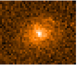
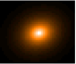
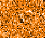
Figure 1: Thumbnail triplet of one of our galaxies. Original galaxy (left), model fit (middle) and residual image (right).

Galfit calculates the total magnitude, scale length, major axis position angle and axis ratio for each galaxy and generates a triplet of thumbnails - of the original object, the model fit and a residual image (see Fig. 1). After the profile fitting, we calculated the central surface brightness, $\rm{\mu_{B,0}}$, in units of $\rm{mag\,arcsec^{-2}}$  using equation 1 (derived from Peng et al. 2002), where $m_{B}$ is the apparent, isophotal magnitude in the B-band, $\alpha$ is the disc scale length in pixel, q is the axis ratio and A is the area of one pixel.

$$\mu_{B,0}=m_{B}+2.5log_{{}_{10}}(2\pi\alpha^{2}qA)$$ (1)

The inclination angle, i, was obtained via equation 2 and the inclination corrected central surface brightness, $\rm{\mu_{B,corr}}$, was calculated using equation 3 (O’Neil et al. 1997).

$$i=cos^{-1}(q)$$ (2)

$$\mu_{B,corr}=\mu_{B,0}-2.5\cdot log_{{}_{10}}(cos\,i)$$ (3)

The diameters of our objects were estimated using an analytical approach as shown in equation 4, where ${\mu_{B,lim}}$ is the limiting B-band surface brightness derived by SExtractor, and ${D_{lim}}$ is the diameter in arcsec at ${\mu_{B,lim}}$. The use of a diameter at the faintest detectable surface brightness for a whole survey is only advisable if $\mu_{B,lim}$ does not differ (very) much between the specific exposures. Otherwise, it would lead to very different selection criteria throughout the survey. Our $\mu_{B,lim}$ depends on the weather conditions and the air mass. The mean value and the standard deviation are $\mu_{B,lim}=25.2\pm 0.31\,$$\rm{mag\,arcsec^{-2}}$. Thus, our ${D_{lim}}$ is pretty comparable to the $D_{25}$, the blue isophotal surface brightness at a level of 25 $\rm{mag\,arcsec^{-2}}$  which is used in many other surveys. Note that our diameters are not estimated by eye but are based on our automated search and fitting algorithms.

$$D_{lim}=\frac{2\,\alpha}{1.086}\cdot(\mu_{B,lim}-\mu_{B,0})$$ (4)

3.3 Removal of the higher redshifted galaxies

We want to limit our search to the local ($z\leq 0.1$) universe in order to reduce the influence of the Tolman $(1+z)^{-4}$ dimming (Phillipps et al. 1990) which shifts the central surface brightness of high redshifted galaxies to the surface brightness region occupied by local LSBs. Without redshifts for all galaxies, one needs secondary methods to reject high-z objects. As higher redshifted galaxies usually have smaller apparent angular scales than nearby galaxies, we used a maximum diameter rejection. To define a limiting diameter which rejects most of the high-z HSBs, one needs to know the size distribution of the HSB galaxy population. For this calibration, we used the $\rm{D_{25}}$ of the Nearby Galaxies Catalog (hereafter NBGC) of Tully (1988), for which we assume that its size distribution is representative (at least at the upper end). The NBGC contains 2 367 galaxies up to a heliocentric velocity of $cz<3\,000\,km/s$ (i.e., 40 Mpc using $H_{0}=75\,km\,s^{-1}\,Mpc^{-1}$). 622 galaxies with $cz<1\,000\,km/s$ were excluded to avoid uncertainties due to deviances from the Hubble flow.

Table 2: Contamination (in %) with higher redshifted HSBs for different limiting diameter at several survey limits.

$z_{lim}$	$D_{lim}$
	10″	14″	18″	22″
0.05	89	75	58	42
0.06	82	63	44	27
0.07	75	52	31	16
0.08	66	40	21	10
0.09	58	31	13	6
0.1	50	22	9	4

We converted the absolute size distribution in kpc to an apparent one (in arcsec), by artificially shifting all galaxies to a specific redshift $z_{lim}$. The fraction of galaxies with an apparent diameter exceeding the limiting diameter $D_{lim}$ then gives the possible contamination of galaxies with $z>z_{lim}$. Table 2 shows this contamination for various values of $z_{lim}$ and $D_{lim}$. It is obvious that a too small $D_{lim}$ increases the contamination with high-z HSBs, whereas a too large $D_{lim}$ would severely reject LSBs as their $D_{25}$ is in general approximately two scale lengths smaller than that from HSBs - assuming the same disc scale length (McGaugh & Bothun 1994) and distance distribution for HSBs and LSBs. Using $D_{lim}=18\hbox{${}^{\prime\prime}$}$ seems the best compromise between the two extremes. At an arbitrary survey limit of $z=0.1$, this $D_{lim}$ results in a contamination with high-z HSBs of about 10 %. Nevertheless, the use of a diameter limit acts as a makeshift solution. To really avoid the rejection of LSBs, one needs redshifts for the complete sample.
After the removal of the objects with a diameter smaller than 18^′′, we verified all our remaining objects by a visual inspection. All unsatisfactorily fitted objects and CCD artifacts were rejected. The cleaned catalogue consists of 306 galaxies, of which 174 were also fitted in the R-Band, and of which 148 were previously uncatalogued. An excerpt of the catalogue is given in table 3. The full catalogue is available in electronic form at the CDS via anonymous ftp to cdsarc.u-strasbg.fr.

Table 3: An excerpt of the object catalogue. The full catalogue is electronically available in the online material.

ID	Other ID	${\alpha_{J2000}}$	${\delta_{J2000}}$	$m_{B}$	$\mu_{B,0}$	$\mu_{B,corr}$	$i_{B}$	$\alpha$	b/a	$D_{lim}$	$m_{R}$	$\mu_{R,0}$	$\mu_{R,corr}$	$i_{R}$
(1)	(2)	(3)	(4)	(5)	(6)	(7)	(8)	(9)	(10)	(11)	(12)	(13)	(14)	(15)
TBHD_J220915+1421.6	[ZBS97] A09	22:09:15	+14:21:38	14.0	21.38	22.42	68	19.61	0.38	136.6	13.5	20.55	21.67	69
TBHD_J222047+1414.0	[ZBS97] A13	22:20:47	+14:14:05	15.4	22.27	22.69	47	11.60	0.68	75.0	-	-	-	-
TBHD_J230556+1421.4	UGC 12354	23:05:56	+14:21:27	14.3	20.84	21.84	66	12.74	0.40	100.0	14.2	20.25	21.21	66
TBHD_J225833+1410.4	–	22:58:33	+14:10:24	19.2	22.62	24.16	76	3.96	0.24	19.2	17.9	20.88	22.41	76
TBHD_J214854+1421.0	–	21:48:54	+14:21:20	17.1	23.43	23.62	33	8.18	0.84	22.1	-	-	-	-
TBHD_J213119+1407.7	–	21:31:19	+14:07:43	18.7	23.04	24.05	67	4.61	0.39	22.8	-	-	-	-

Note: (1) IAU conformable identifier; (2) prior identification according to the NED (If blank, the galaxy was previously uncatalogued); (3) right ascension (J2000) in hours, minutes, seconds; (4) declination (J2000) in degree, minutes, seconds; (5) apparent, isophotal magnitude in the B-band; (6) B-band central surface brightness in $\rm{mag\,arcsec^{-2}}$; (7) inclination corrected central B-band surface brightness in $\rm{mag\,arcsec^{-2}}$; (8) inclination angle from B-band data in degree; (9) B-band scale length in arcsec; (10) axis ratio derived from the B-band data; (11) object diameter in arcsec in the B-band data at the limiting surface brightness; (12) apparent, isophotal magnitude in the R-band; (13) R-band central surface brightness in $\rm{mag\,arcsec^{-2}}$; (14) inclination corrected central R-band surface brightness in $\rm{mag\,arcsec^{-2}}$; (15) inclination angle from R-band data in degree. For the objects of which we have no R-band data , Cols. 12-15 are left blank.

4 The detection efficiency tested using artificial objects

We tested our detection efficiency and the effect of our selection criteria like CLASS_STAR $\leq$ 0.1, FLAGS $<$ 3, $D_{lim}\geq\,18\hbox{${}^{\prime\prime}$}$, and masking of blooming regions with large samples of artificial galaxies. We created these objects using the gallist task in IRAF and added about 85 000 galaxies of varying parameters in our B-band images using the IRAF task mkobject. The galaxies cover a large parameter space in total magnitude ($12\leq m_{B}\leq 22\,mag$) and central, for inclination uncorrected, surface brightness ($18.5\leq\mu_{B,0}\leq 26\,$$\rm{mag\,arcsec^{-2}}$). We ensured that each bin (the bin size is 0.25 mag and $\rm{mag\,arcsec^{-2}}$, respectively) in both parameters contains at least 10-20 objects, and most bins (especially in regions where the detection efficiency drops) contain more than 50 galaxies (the mean value is 90). The input parameters from gallist are magnitude, eradius, position angle and axis ratio. The eradius is related to the scale length $\rm{\alpha}$ by equation 5.

$$eradius=2\alpha\,log_{10}(2)$$ (5)

The object detection was done by SExtractor using the same parameters as on the original science frames. The original objects were then excluded from the catalogues so that the catalogues contain only the new, artificial galaxies.
After the removal of flagged objects (either with the blooming flag or with FLAGS $\geq$ 3), the remaining objects were fed into Galfit (again with the same parameters as in the survey) and the size of each object was calculated. Due to the huge numbers of galaxies, we refrained from checking each object visually and simply rejected all objects which could not be fitted by Galfit without interaction. For the remaining galaxies, we adopted the same diameter criterion as for our original data and rejected all galaxies smaller than 18^′′  in diameter.

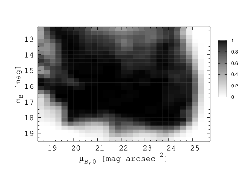
Figure 2: Surface plot of the detection efficiency in respect of magnitude and surface brightness. The dip in the efficiency for bright objects is mainly due to the expansion of these objects into areas affected with blooming which led to their rejection.

4.1 The detection efficiency for our data

The surface plot in Fig. 2 shows the fraction of the recovered objects in respect of the input objects in the same magnitude/surface brightness bin. The bin size is 0.25 mag and $\rm{mag\,arcsec^{-2}}$  respectively. The detection efficiency exceeds the 90 % level for a large part of the parameter space ($\rm{15.5\la m_{B}\la 18}$ mag & $\rm{20.5\la\mu_{B,0}\la 24}$ $\rm{mag\,arcsec^{-2}}$). Nevertheless, our sample of real galaxies contains only few objects with $\rm{\mu_{B,0}\la 23\,mag\,arcsec^{-2}}$, as these objects need quite large scale length to reach a $\rm{D_{lim}>18\hbox{${}^{\prime\prime}$}}$. Objects with $\rm{\mu_{B,0}\la 19.5\,mag\,arcsec^{-2}}$ look rather star-like and were partly rejected due to ${\rm CLASS\_STAR\geq 0.1}$. Also rejected were the bright objects with $\rm{20.5\leq\mu_{B,0}\leq 23.5\,}$$\rm{mag\,arcsec^{-2}}$  which, due to their large sizes, have a higher probability of being located in an area affected by blooming.
The drop-off towards faint surface brightnesses is quite sharp and rather independent from the total magnitude. In contrast, the decline in magnitude direction is more dependent on the surface brightness. The point at which the decline occurs moves slightly towards fainter magnitudes if one goes to fainter surface brightnesses, as the scale length for these artificial galaxies is larger and they can achieve a diameter larger than 18^′′  before disappearing into the noise.

4.2 The detection efficiency of the real galaxies

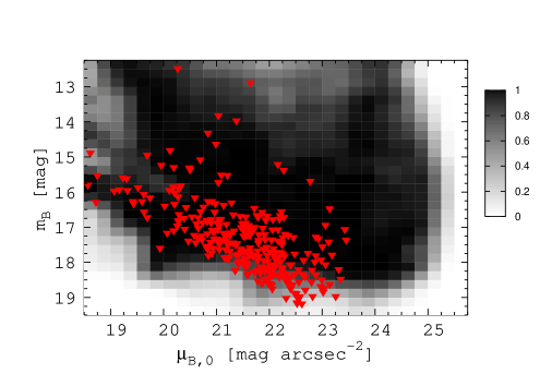
Figure 3: The same surface plot as in Fig. 2, but we additionally inserted the detected objects into this plot (red triangles). As one can see, the real galaxies do not cover the whole area which is accessible with our search methods, and most objects lay in regions with high detection efficiency.

Figure 3 shows the same as Fig. 2, with the addition of real objects from our sample (red triangles). As both data sets underwent the same analysis and selection, no systematic difference should arise between them. The real galaxies are mostly located in a well defined region of the diagram, even though the parameter space covered by the artificial galaxies is quite large. This is due to the fact that the parameter range of our artificial galaxies is purely theoretical, and, e.g., galaxies with a scale length of 50″  should be rather rare. Nevertheless, most of the found objects are located in regions with a high detection efficiency, where our survey is expected to be quite complete. For faint objects with $\rm{m_{B}>18.5\,mag}$, the detection efficiency drops below 50 % and thus our galaxy counts for these objects give only lower limits, which could be more than a factor of 2 too low. Analogous to the trends in Cross & Driver (2002) and Driver et al. (2005), we can see a general trend towards fainter central surface brightnesses if one goes to fainter total magnitudes.

5 Results

5.1 The number density

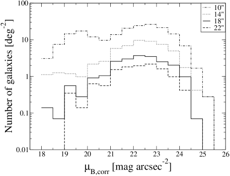
Figure 4: The number of galaxies per deg² per inclination corrected central surface brightness bin (bin size 0.5 $\rm{mag\,arcsec^{-2}}$) for samples with different limiting diameters is shown on a logarithmic scale. The limiting diameter has a strong influence on the number density.

Figure 4 shows the distribution of the inclination corrected central surface brightness ($\mu_{B,corr}$) for our final sample ($D_{lim}>18\hbox{${}^{\prime\prime}$}$) and for other limiting diameter. A smooth transition can be seen between galaxies of high and low surface brightness, at $\rm{\mu_{B,corr}=22.5\,}$$\rm{mag\,arcsec^{-2}}$. For smaller $D_{lim}$, both the number density and the contamination with high redshifted galaxies are higher. Setting an arbitrary survey limit at $z=0.1$ and using the assumptions based on the NBGC as discussed in Section 3.3, a $D_{lim}$ of 10^′′  leads to a 50 % contamination of galaxies with $z\la 0.1$, whereas at $D_{lim}=18\hbox{${}^{\prime\prime}$}$ this contamination is reduced to only 9 % (see Table 2).
The objects in the brightest bins ($\rm{\mu_{B,corr}<20\,mag\,arcsec^{-2}}$) are mainly spiral galaxies with strong bulges, which are responsible for their high central surface brightnesses, since we did not make any decomposition but fitted a single profile to our galaxies.
We classified 130 galaxies (42 %) as LSBs. Even if we restrict the survey to $z<0.1$, cosmological dimming has to be taken into account, as at $z=0.1$ a galaxy is dimmed about 0.4 $\rm{mag\,arcsec^{-2}}$. To avoid an overestimation of LSBs, we used the most extreme case that all galaxies are located at $z=0.1$, which shifts our LSB selection criterion from 22.5 $\rm{mag\,arcsec^{-2}}$  to 22.9 $\rm{mag\,arcsec^{-2}}$. If we adopt this criterion, 96 (30 %) of our galaxies are LSBs, which indicates that these objects contribute substantially to the local galaxy number density, since this number is clearly a lower limit.
Our results of 30-40 % are in agreement with other surveys. Minchin et al. (2004) estimated the contribution (by numbers) of low surface brightness galaxies to gas-rich ($M_{HI}>10^{8}\,M_{\odot}$) galaxies to be 50-60 %, and 50 % of the galaxies in the sample of Spitzak & Schneider (1998) have a central disc surface brightness fainter than 22.5 $\rm{mag\,arcsec^{-2}}$  in the B-band and are therefore LSBs. In the sample of Driver et al. (2005), 26 % of the galaxies have an effective surface brightness fainter than 23.6 $\rm{mag\,arcsec^{-2}}$. According to Cross et al. (2001), this corresponds to a central surface brightness of 22.5 $\rm{mag\,arcsec^{-2}}$.

5.2 Comparison with other optical surveys

In the following, we compare the surface brightness distribution of our survey with that from two other optical surveys. The first one is the Texas-Survey by O’Neil et al. (1997, OBC97 hereafter) and the second one is a very deep search for LSBs in the HDF–S (Haberzettl et al. in press., HBDP hereafter).

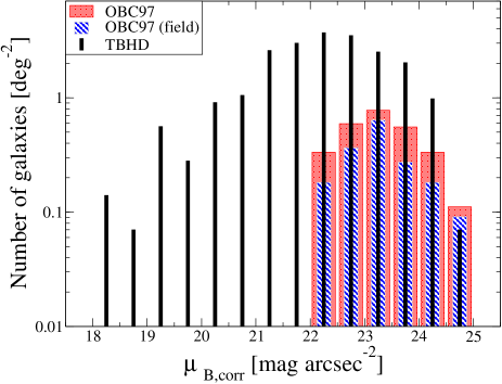
Figure 5: The SB distribution for our survey (TBHD) and for OBC97 and the field sample of OBC97. To make a comparison of the two surveys easier, the same diameter limit was applied to all samples (see text).

5.2.1 Texas-Survey (OBC97)

The Texas-Survey was targeted on cluster and field environments and covered an area of 27 deg². The original catalogue contained 127 galaxies which were visually selected. The selection criteria of OBC97 were $\rm{\mu_{B,0}\geq\,22\,mag\,arcsec^{-2}}$ and $R_{27}\ga 13\aas@@fstack{\prime\prime}2$. The size estimation was also done visually, and the limiting surface brightness of the survey is $\rm{\mu_{lim}\approx\,27\,mag\,arcsec^{-2}}$. It is not straightforward to compare two surveys with such differences in the object detection, size estimation, and adopted diameter limits. To make the comparison easier, we compared samples with almost identical diameter limits, and instead of using $R_{27}\ga 13\aas@@fstack{\prime\prime}2$ we used $D_{25}>18\hbox{${}^{\prime\prime}$}$, which matches our diameter criterion. Moreover, we made an additional analysis using only the field objects of OBC97, as galaxy clusters typically show a different galaxy population than field galaxies (Binggeli et al. 1987).
The SB distribution of our survey (referred to as TBHD) and of OBC97 and the field sample of OBC97 is shown in Fig. 5. The decline of the OBC97 sample in the $\rm{22\leq\mu_{B,corr}\leq 22.5\,mag\,arcsec^{-2}}$ bin is a result of their upper SB selection limit. Between $\rm{22.5\leq\mu_{B,corr}\leq 24.5\,mag\,arcsec^{-2}}$, our number density is higher than that of OBC97 (in average 6.5 times as high as the field sample and 3.9 times as high as the field+cluster sample). The differences in the number density and the survey areas are high enough to exclude cosmic variance (our survey area: 14.3 deg², OBC97: 27 deg², of which $\approx\,$11 deg² is field). It may be possible that the differences originate from the diverse methods for object detection and size estimation (which is important if using a diameter limit). If this were true, it would show that automated methods for object detection and size estimation increase the galaxy number density significantly - in any case, it emphasises that galaxy catalogues created by automated methods are at least as complete as visually selected ones.
The relatively low (compared to OBC97) number density in the faintest populated bin may be a result from our automated star-galaxy separation which becomes difficult and partially uncertain for low S/N objects.

5.2.2 HDF–S (HBDP)

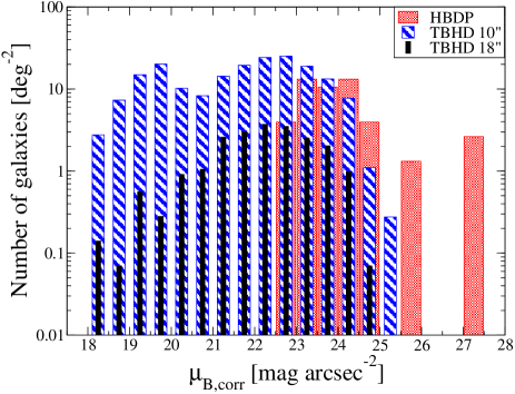
Figure 6: As Figure 5; the SB distribution of HBDP and for two diameter limits of our survey (TBHD).

Figure 6 shows the comparison between our survey and the sample from HBDP. The survey which HBDP used has a limiting surface brightness of $\rm{\mu_{B_{w}}\approx 29\,mag\,arcsec^{-2}}$ in the $B_{w}$-band, which is slightly broader than Johnson-B. HBDP estimate the $<\mu_{B_{w}}-\mu_{B}>$ correction term for their SB as $0.41\pm 0.28$ $\rm{mag\,arcsec^{-2}}$ and adopted this offset to their objects without data in Johnson-B. For Fig. 6 we used the inclination corrected central surface brightnesses in Johnson-B. The object detection of HBDP was done by SExtractor and they included only galaxies in their catalogue with $\mu_{B_{w}}>22\,mag\,arcsec^{-2}$ and a visually estimated diameter at the limiting isophote of more than 10$\aas@@fstack{\prime\prime}$8. Additionally to the SExtractor search, HBDP used a median filter method adopted from Armandroff et al. (1998). HBDP removed all objects found by SExtractor from the original data and filtered the source-free image with a median filter with a kernel size of 25 pixel (10$\aas@@fstack{\prime\prime}$8). With this method, they detected the three extreme LSB objects which populate the bins with $\rm{\mu_{B,corr}>25.5\,mag\,arcsec^{-2}}$.
As a comparison of a $D_{29}>10\aas@@fstack{\prime\prime}8$ sample with a $D_{25}>18\hbox{${}^{\prime\prime}$}$ sample is not straightforward, we added a third sample with $D_{25}>10\hbox{${}^{\prime\prime}$}$ to Fig. 6, although even the latter limit is clearly different from $D_{29}>10\hbox{${}^{\prime\prime}$}$. Although HBDP measure their diameters at a four magnitudes fainter SB level, the number density of their sample for surface brightnesses between $\rm{23\leq\mu_{B,corr}\leq 24.5\,mag\,arcsec^{-2}}$ is only as high as that of our $D_{25}>10\hbox{${}^{\prime\prime}$}$ sample. If HBDP had also used $D_{25}>10\hbox{${}^{\prime\prime}$}$ for their selection, their number density would have dropped by a factor of more than 2.5 and be significantly below ours.
Cosmic variance and low number statistics may play a role here as the area of HBDP and their number of galaxies are quite small (37 galaxies in 0.76 deg²). Another possible reason may again be the different methods for the size estimation. It is possible that the eye underestimates galaxy sizes, which, when using a diameter limit would lead to a lower number density.
This hypothesis is supported by first tests we made using a SExtractor-based search and a galaxy fitting using Galfit on the HDF–S image of HBDP. Adopting their selection criteria ($\rm{\mu_{B_{w}}>22\,mag\,arcsec^{-2},D_{lim}>10\aas@@fstack{\prime\prime}8}$) and estimating the size analytically instead of visually increased the number of galaxies matching these criteria significantly (up to a factor of $\approx$ 5).

Table 4: Optical and HI parameter for the galaxies found in both our survey and in the AHISS.

ID	${\alpha_{J2000}}$	${\delta_{J2000}}$	$m_{B}$	$\mu_{B,0}$	$\mu_{B,corr}$	$i_{B}$	$D_{lim}$	$M_{B}^{b}$	log $M_{HI}$	$M_{HI}/L_{B}^{b,i}$
(1)	(2)	(3)	(4)	(5)	(6)	(7)	(8)	(9)∗	(10)∗	(11)∗
ZBS97  A03	21:49:27	+14:14:00	15.7	22.77	23.24	50	50.61	-15.8	9.1	3.84
ZBS97  A04-1	21:59:05	+14:14:19	17.4	23.01	23.28	39	27.61	-13.6	8.0	1.99
$\rm{[ZBS97\,A04}$-$\rm{2]}$	21:58:35	+14:06:53	14.9	22.03	22.25	35	75.07	-16.3	9.2	2.81
ZBS97  A09	22:09:15	+14:21:38	14.0	21.38	22.42	68	136.56	-16.7	8.8	0.64
ZBS97  A10	22:58:10	+14:18:31	12.9	21.65	21.70	18	153.47	-18.2	8.9	0.27
ZBS97  A11	23:01:18	+14:20:22	13.8	21.04	22.59	76	173.77	-17.5	9.5	1.54
$\rm{[ZBS97\,A12]}$	23:26:09	+14:15:46	19.6	23.23	23.94	58	8.71	-12.7	7.9	4.21
ZBS97  A13	22:20:47	+14:14:05	15.4	22.27	22.69	47	75.01	-17.5	9.3	1.31
ZBS97  A14	23:36:37	+14:09:25	15.2	22.16	22.90	60	81.10	-17.8	9.7	1.94
ZBS97  A15	00:11:08	+14:14:22	16.8	22.19	22.99	61	35.98	-12.2	7.3	1.57
ZBS97  A17	00:20:09	+14:17:28	16.4	21.14	21.84	58	34.20	-16.7	9.2	2.02
$\rm{[ZBS97\,A18]}$a	00:24:30	+14:16:15	16.6	21.71	23.11	74	51.40	-16.9	8.5	0.26
ZBS97  A19	00:28:03	+14:18:07	17.2	21.91	22.08	31	23.36	-15.4	8.9	3.48
$\rm{[ZBS97\,A21]}$	00:44:24	+14:17:55	17.5	20.95	21.26	41	13.54	-15.1	8.3	0.83

Note: (1) identifier according to ZBS97; (2) right ascension (J2000) in hours, minutes, seconds; (3) declination (J2000) in degree, minutes, seconds; (4) apparent, isophotal magnitude in the B-band; (5) B-band central surface brightness in $\rm{mag\,arcsec^{-2}}$; (6) inclination corrected central B-band surface brightness in $\rm{mag\,arcsec^{-2}}$; (7) the inclination angle obtained from the B-band data in degree; (8) object diameter in arcsec in the B-band data at the limiting surface brightness; (9) Absolute B-band magnitude corrected for Galactic extinction, not corrected for inclination effects; (10) Logarithm of HI mass in solar masses; (11) Ratio of HI mass to B luminosity in solar units. The luminosity is corrected for inclination effects using the method of Tully et al. (1998).
^∗ Columns 9-11 and their description are taken from Zwaan (2000).

5.3 Comparison with the AHISS

Zwaan et al. (1997, ZBS97 hereafter) used the AHISS to search for extragalactic sources and found 66 galaxies up to a velocity of ${\rm cz=7400\,km\,s^{-1}}$ in an area of 65 deg², of which 51 were detected by the main beam of the Arecibo telescope, which covered an area of 15 deg². The telescope sidelobes are considerably less sensitive than the main beam, and their sensitivity is uncertain due to temperature dependencies and asymmetries (Schneider et al. 1998). Thus, we will henceforth restrict our comparison to the main beam of the Arecibo telescope, unless otherwise stated. The AHISS is until now the most sensitive blind HI survey in terms of HI mass and flux limits. The average noise level of the AHISS is 0.75 mJy for a velocity resolution of 16 km s^-1 and the HI mass limit at the full survey depth is $\rm{1.5\,\times\,10^{8}\,h^{-2}\,M_{\odot}}$ (ZBS97) - assuming a profile width of $\rm{85\,km/s}$ and a sigma level of 5.
For the direct cross-check of the detections in the blind AHISS with those in our survey, we included also the sidelobe detections. The AHISS contains 15 objects in the area which is covered by our survey. All 15 sources were found in our images by our automated routines, but the five whose names appear in square brackets in Table 4 were rejected during the data processing. The optical and HI properties of 14 of these galaxies are given in Table 4. Of the five rejected galaxies, three are affected by blooming (A04-2, A18, A20) - the latter so badly that it was omitted from Table 4, a fourth (A21) has a $D_{lim}$ of only 13$\aas@@fstack{\prime\prime}$5, and a fifth (A12) which is quite faint and small is located in an area with low S/N and was given a CLASS_STAR parameter of 0.31 by SExtractor.
A comparison of the main beam sample of ZBS97 with our sample allows more general comments. The galaxy number density in the main beam of the AHISS is 3.4 per deg² (51 in 15 deg²), whereas ours is 21.4 per deg² (306 in 14.3 deg²). Thus, our number density (for HSBs + LSBs) is a factor of 6.3 higher than that from the AHISS. If we make this comparison for the LSB samples only, the difference in number density decreases. Taking the surface brightness values of the AHISS sample from Zwaan (2000), and using ${\rm\mu_{B,corr}>22.9\,mag\,arcsec^{-2}}$ to define LSBs in our catalogue (i.e., adopting a cosmological dimming of 0.4 $\rm{mag\,arcsec^{-2}}$  for our estimated survey limit at $z=0.1$), the difference decreases to a factor of four (number density TBHD 6.7, AHISS 1.67 galaxies per deg²). If we neglect all cosmological corrections and use ${\rm\mu_{B,corr}>22.5\,mag\,arcsec^{-2}}$, the number densities differ by a factor of 5.5. If dimming could be applied correctly (i.e., when the redshifts for all objects are known), it is likely that the factor will lie between 4 and 5.5.
It is not unexpected that the number density of our optical survey is significantly larger than that of the AHISS, as the AHISS has a limited velocity range. To estimate to what extent the velocity range contributes to this differences, one would need redshifts for all (or at least for most) of the optically selected galaxies.
The difference in the number densities is smaller for the LSB subsample (4-5.5) than for the full sample (6.3). This trend may have two reasons. Firstly, HI surveys may have a smaller bias against the detection of LSBs as optical surveys (regardless of the fact that all sources detected by AHISS have optical counterparts). Secondly, our selection criteria - especially the diameter limit of $D_{lim}\approx D_{25}>18\hbox{${}^{\prime\prime}$}$ - may cause the rejection of LSBs. However, using a smaller diameter limit will artificially increase the number of LSBs due to cosmologically dimmed HSB galaxies. Thus, without spectroscopic follow-up observations, diameter-limited catalogues created from optical surveys will either be strongly biased against LSBs, or contaminated with high redshifted HSBs.

6 Conclusions

We performed optical follow-up observations of a part of the AHISS, and detected optical counterparts of all HI detections. We estimated the detection efficiency of our survey using large samples of artificial galaxies. The comparison of our survey with two other optical surveys indicates that an automated search algorithm and an analytical size estimation may increase the number of galaxies per deg² compared to catalogues based on visual estimates. We show that diameter-limited catalogues created by automated routines are at least as complete as visually created ones.
Although our number density is higher than that of the AHISS (mainly due to the limited velocity range of AHISS), the fraction of LSBs in the AHISS is higher than in our survey (30-42 % in TBHD vs. 49 % in AHISS). We suggest that this is caused by our relatively large diameter limit, which reduces the contamination of the sample with cosmologically dimmed higher redshifted galaxies, but also rejects local LSBs. In order to reduce this bias against the selection of LSBs in optical surveys one needs redshifts for the whole sample. For a given observing time, optical surveys are despite all drawbacks best suited to detect a large number of galaxies. The information which optical surveys provide on detected galaxies is, however, fundamentally different from that of HI surveys. The radial velocity information inherent to HI surveys allows a direct estimation of the volume density and the rejection of high-z HSBs. However, they will miss the gas-poor LSBs and can only probe a limited velocity range. With current telescopes, only very massive galaxies ($M_{HI}>10^{10}\,M_{\odot}$) can be detected beyond 10 000 km s^-2. For example, the 6$\sigma$ HI mass limit of the ALFALFA survey will be $\sim 9.5\,\times\,10^{9}\,M_{\odot}$ at $cz=10\,000\,km/s$ Giovanelli et al. (2005). Thus, HI and optical surveys are complementary, as are the differences between the samples of LSB galaxies they detect. Therefore, we especially need extremely deep surveys of both kinds to extend our - still limited - knowledge about LSBs. That we have not yet reached the end can e.g., be seen from the very deep HBDP optical survey.