Binary Stars in the Orion Nebula Cluster

We report on a high-spatial-resolution survey for binary stars in the periphery of the Orion Nebula Cluster, at 5–15 arcmin (0.65 – 2 pc) from the cluster center. We observed 228 stars with adaptive optics systems, in order to find companions at separations of $0\aas@@fstack{\prime\prime}13$ – $1\aas@@fstack{\prime\prime}12$ (60 – 500 AU), and detected 13 new binaries. Combined with the results of Petr (1998), we have a sample of 275 objects, about half of which have masses from the literature and high probabilities to be cluster members. We used an improved method to derive the completeness limits of the observations, which takes into account the elongated point spread function of stars at relatively large distances from the adaptive optics guide star. The multiplicity of stars with masses $>2\,M_{\sun}$ is found to be significantly larger than that of low-mass stars. The companion star frequency of low-mass stars is comparable to that of main-sequence M-dwarfs, less than half that of solar-type main-sequence stars, and 3.5 to 5 times lower than in the Taurus-Auriga and Scorpius-Centaurus star-forming regions. We find the binary frequency of low-mass stars in the periphery of the cluster to be the same or only slightly higher than for stars in the cluster core ($<$3 arcmin from $\theta^{1}$C Ori). This is in contrast to the prediction of the theory that the low binary frequency in the cluster is caused by the disruption of binaries due to dynamical interactions. There are two ways out of this dilemma: Either the initial binary frequency in the Orion Nebula Cluster was lower than in Taurus-Auriga, or the Orion Nebula Cluster was originally much denser and dynamically more active.

1 Introduction

Over the past decade it has become clear that stellar multiplicity can be very high among young low-mass stars, with companion star frequencies close to 100 % for young stars in well-known nearby star-forming T associations (Leinert et al. Leinert93 (1993), Ghez et al. Ghez93 (1993), Ghez et al. Ghez97 (1997), Duchêne Duchene99a (1999)). Thus, our current understanding is that star formation resulting in binary or multiple systems is very common, if not the rule. However, the multiplicity of low-mass main-sequence field stars is significantly lower, only $\sim 55\,\%$ for solar-type stars (Duquennoy & Mayor DM91 (1991)), and $\sim 35$ to $42\,\%$ for M-dwarfs (Reid & Gizis RG97 (1997), Fischer & Marcy FM92 (1992)).

On the other hand, high binary frequencies are not observed among low-mass stars in stellar clusters. Binary surveys in the center of the young Trapezium Cluster (e.g. Prosser et al. Prosser94 (1994), Padgett et al. Padgett97 (1997), Petr et al. Petr98 (1998), Petr PetrPhD (1998), Simon et al. Simon99 (1999), Scally et al. Scally99 (1999), McCaughrean MJM2001 (2001)), which is the core of the Orion Nebula Cluster (ONC); and in the young clusters IC 348 and NGC 2024 (Duchêne et al. Duchene99b (1999), Beck et al. BeckSC03 (2003), Liu et al. Liu2003 (2003), Luhmann et al. Luhman2005 (2005)), as well as those in older ZAMS clusters (Bouvier et al. Bouvier97 (1997), Patience et al. Patience98 (1998)) show binary frequencies that are comparable to that of main-sequence fields stars, i.e. lower by factors of 2 – 3 than those found in loose T associations. The reason for this discrepancy is still unclear. Theoretical explanations include:

• Disruption of cluster binaries through stellar encounters.

  Kroupa (Kroupa95 (1995)) and Kroupa et al. (Kroupa99 (1999)) suggested that dynamical disruption of wide binaries (separations ${}>100\rm\,AU$) through close stellar encounters decreases the binary fraction in clusters. If the primordial binary output from the star-formation process is the same in dense clusters and in loose T associations, then the number of “surviving” binaries depends on the number of interactions of a binary system with other cluster members that occurred since the formation of the cluster. This number is derived from the age of the cluster divided by the typical time between stellar interactions. The typical time between interactions is inversely proportional to the stellar volume density of the cluster (Scally et al. Scally99 (1999)), thus binaries at the cluster center get destroyed more quickly than those at larger radii. Observing various subregions of a single star-forming cluster representing different stellar number densities will therefore reveal different binary fractions if this mechanism is dominant in the evolution of binary systems.

• Environmental influence on the initial binary fraction.

  Durisen & Sterzik (DurSterz94 (1994)) and Sterzik et al. (Sterzik2003 (2003)) suggested an influence of the molecular cores’ temperature on the efficiency of the fragmentation mechanism that leads to the formation of binaries. Lower binary fractions are predicted in warmer cores. Assuming the ONC stars formed from warmer cores than the members of the Taurus-Auriga association, less initial binaries are produced in this scenario. Observations of different subregions of the ONC should therefore reveal the same (low) binary frequency (if the molecular cores in these regions had the same temperature – a reasonable, though unverifiable assumption).

These theoretical concepts make different predictions that can be tested observationally. Indeed, measuring the binary fraction as a function of distance to the cluster center will provide important observational support for one or the other proposed theoretical explanation.

Table 1: Fields observed for this work. Name is the designation in Jones & Walker (JW88 (1988)) or Parenago (Parenago (1954)) of the central star that was used to guide the adaptive optics system, $r$ is the distance to $\theta^{1}$C Ori. In the last columns, we list the number of stars actually observed in this field and the date(s) of observation.

Name	$\alpha_{2000}$	$\delta_{2000}$	$r$ [′]	Targets	Obs. Date
JW0005	5:34:29.243	-5:24:00.37	11.8	6	09.12.2001
JW0014	5:34:30.371	-5:27:30.46	12.2	2	11.12.2001
JW0027	5:34:34.012	-5:28:27.72	11.8	4	11.12.2001
JW0045	5:34:39.774	-5:24:28.27	9.2	4	10.12.2001
JW0046	5:34:39.917	-5:26:44.70	9.7	5	10.12.2001
JW0050	5:34:40.831	-5:22:45.07	8.9	1	11.12.2001
JW0060	5:34:42.187	-5:12:21.55	14.0	2	10.12.2001
JW0064	5:34:43.496	-5:18:30.01	9.6	3	17.02.2002
JW0075	5:34:45.188	-5:25:06.33	8.0	7	09.12.2001
JW0108	5:34:49.867	-5:18:46.79	8.1	3	10.12.2001
JW0116	5:34:50.691	-5:24:03.25	6.5	5	11.12.2001
JW0129	5:34:52.347	-5:33:10.38	11.5	4	10.12.2001
JW0153	5:34:55.390	-5:30:23.42	8.8	2	17.02.2002
JW0157	5:34:55.936	-5:23:14.58	5.1	4	17.02.2002
JW0163	5:34:56.560	-5:11:34.84	12.8	3	11.12.2001
JW0165	5:34:56.601	-5:31:37.48	9.6	2	11.12.2001
JW0221	5:35:02.202	-5:15:49.28	8.4	4	11.12.2001
JW0232	5:35:03.090	-5:30:02.27	7.5	5	09.12.2001
JW0260	5:35:04.999	-5:14:51.45	9.0	3	11.12.2001
JW0364	5:35:11.455	-5:16:58.33	6.5	13	09.12.2001
JW0421	5:35:13.706	-5:30:57.76	7.6	5	11.12.2001
					17.02.2002
JW0585	5:35:18.275	-5:16:37.83	6.8	17	09.12.2001
JW0666	5:35:20.936	-5:09:15.92	14.2	8	09.12.2001
JW0670	5:35:21.043	-5:12:12.52	11.2	2	17.02.2002
JW0747	5:35:23.929	-5:30:46.82	7.6	5	10.12.2001
JW0779	5:35:25.417	-5:09:48.98	13.8	11	09.12.2001
JW0790	5:35:25.953	-5:08:39.42	14.9	5	10.12.2001
JW0794	5:35:26.121	-5:15:11.27	8.5	6	09.12.2001
JW0803	5:35:26.565	-5:11:06.84	12.5	4	10.12.2001
JW0804	5:35:26.666	-5:13:13.97	10.5	1	17.02.2002
JW0818	5:35:27.716	-5:35:19.01	12.3	2	11.12.2001
JW0866	5:35:31.077	-5:15:32.23	8.7	4	09.12.2001
JW0867	5:35:31.116	-5:18:55.12	5.8	3	09.12.2001
JW0873	5:35:31.521	-5:33:07.91	10.5	6	11.12.2001
JW0876	5:35:31.627	-5:09:26.88	14.4	3	11.12.2001
JW0887	5:35:32.487	-5:31:10.05	8.8	1	17.02.2002
JW0915	5:35:35.509	-5:12:19.38	12.0	2	11.12.2001
JW0928	5:35:37.385	-5:26:38.20	6.2	4	10.12.2001
JW0950	5:35:40.519	-5:27:00.48	7.0	4	11.12.2001
JW0959	5:35:42.019	-5:28:10.95	8.0	5	10.12.2001
JW0963	5:35:42.528	-5:20:11.73	7.3	5	09.12.2001
JW0967	5:35:42.803	-5:13:43.69	11.7	1	17.02.2002
JW0971	5:35:43.476	-5:36:26.22	14.7	4	10.12.2001
JW0975	5:35:44.558	-5:32:11.40	11.3	3	11.12.2001
JW0992	5:35:46.845	-5:17:54.69	9.4	6	09.12.2001
JW0997	5:35:47.326	-5:16:56.01	10.1	4	11.12.2001
JW1015	5:35:50.509	-5:28:32.56	10.0	2	10.12.2001
JW1041	5:35:57.831	-5:12:52.17	14.8	1	17.02.2002
Par1605	5:34:47.201	-5:34:16.76	13.1	3	10.12.2001
Par1744	5:35:04.822	-5:12:16.61	11.5	4	11.12.2001
Par2074	5:35:31.223	-5:16:01.54	8.2	13	09.12.2001
					17.02.2002
Par2284	5:35:57.539	-5:22:28.21	10.3	2	17.02.2002

Figure 1: Fields observed in this work (large boxes) and Petr (PetrPhD (1998), small boxes in the central region). Dots mark the positions of all stars in the list of Jones & Walker (JW88 (1988)), these are not the stars observed by us. The stars used to guide the adaptive optics are marked by star symbols and their number in Jones & Walker or Parenago (Parenago (1954)). The large boxes show the areas where we selected our target stars. These fields were not fully covered by our observations, we only observed stars visible in the 2MASS quicklook images (see Sect. 2).

The ONC is the best target for this study. Its stellar population is very well studied, more than 2000 members are known from extensive near-infrared and optical imaging (Hillenbrand H97 (1997), Hillenbrand & Carpenter 2000). To date, binary surveys of the cluster have focused on the central 0.25 pc core, where the stellar density reaches as high as $2$ – $5\times 10^{4}\rm\,pc^{-3}$ (McCaughrean & Stauffer MJMStau94 (1994), Hillenbrand & Hartmann Hillenbr98 (1998)). The typical time between interactions for a binary with a separation of 250 AU ($\sim 0\aas@@fstack{\prime\prime}5$ at the distance of the ONC) in the core is $\sim 1\rm\,Myr$, the age of the cluster. Therefore, most 250 AU binaries are likely to have experienced at least one close encounter. However, for the observed stellar density distribution of the cluster, which can be described by an isothermal sphere with $n\propto r^{-2}$ outside 0.06 pc (Bate et al. Bate98 (1998)), the volume density at $\sim$ 1 pc distance from the center ($\sim 8\arcmin$ at the distance of the ONC) is roughly $200\rm\,pc^{-3}$ and the interaction timescale for our 250 AU binary would be $>250$ Myr, hundreds of times the age of the cluster. We also know that dynamical mass segregation in the cluster has not yet occurred (Bonnell & Davies BonnellDavies98 (1998)) and that the ejection of single stars from the inner parts of the cluster (where many binary disruptions have already occurred) has not been efficient to populate the outer regions if the whole cluster is roughly virialized (Kroupa et al. Kroupa99 (1999)). For these reasons, the binary fraction in the outer parts of the ONC is unlikely to have been modified by the dynamical evolution of the cluster, and should be the intrinsic value resulting from the fragmentation process, while the binary frequency of stars in the cluster core has already been lowered by dynamical interactions.

We have measured the frequency of close binaries among stars in a number of fields in the outer part of the ONC using adaptive optics imaging in the K-band. The results we obtain in this survey for the outskirts of the Orion Nebula Cluster will be compared with a similar study of the ONC core, carried out by Petr et al. (Petr98 (1998)) and Petr (PetrPhD (1998)). Since the same instrument and observing strategy was used, we incorporate their results, and constrain the radial distribution of the binary frequency from the ONC core to the cluster’s periphery.

2 Observations

Since our study concentrates on the detection of close binary or multiple stars with sub-arcsecond separations, it is necessary to use an imaging technique that provides the required performance in terms of high spatial resolution and sensitivity. Therefore, we carried out adaptive optics near-infrared imaging at ESO’s 3.6 m telescope and the Keck II telescope using their respective adaptive optics instruments.

The choice of our target fields in the Orion Nebula cluster was mainly guided by two criteria. First, the necessity of having a nearby (within $\sim 30\arcsec$) optically bright reference star that controls the wavefront correction in order to obtain (nearly) diffraction-limited images. Second, the fields should be located at radii larger than 5arcmin from the cluster center.

Based on these criteria, we searched the catalogues of Jones & Walker (JW88 (1988), JW hereafter) and Parenago (Parenago (1954)) for stars with $\rm I<12.5^{m}$ and located at radii of 5–15 arcmin (0.65 – 2 pc) from the cluster center. The resulting list contains 57 objects, 52 of them were observed in the course of this project (see Tab. 1 and Fig. 1). The remaining fields had to be omitted because of time constraints.

Since the field of view’s of the used instruments are at most $12\aas@@fstack{\prime\prime}8\times 12\aas@@fstack{\prime\prime}8$, it would have been very inefficient to completely survey the fields around each guide star. Instead, we used quicklook-images from the 2MASS database to find stars within $30^{\prime\prime}$ from the guide stars, and pointed only at these sources. Therefore, we did not observe all stars within $30\arcsec$ from a guide star, but only those visible in 2MASS quicklook-images. The 2MASS survey is complete to at least $\rm K_{s}=14^{\rm mag}$ (except in crowded regions), so we can be sure all stars down to this magnitude are visible in the quicklook-images and have been observed by us. Our estimated masses (Sect. 4.2) indicate that this probably already includes a few brown dwarfs, so the number of interesting targets (low-mass stars) missed by this procedure is negligible.

Figure 2 shows as an example the 2MASS quicklook-image of the region around JW0971, and our AO-corrected images.

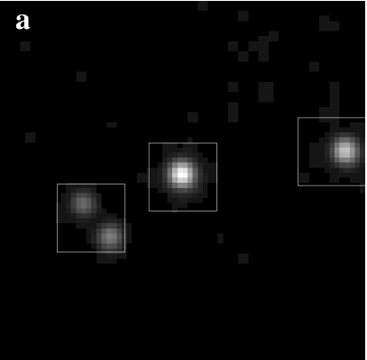
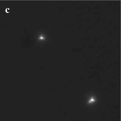
Figure 2: The field around JW0971 as an example of our observations. North is up and East is to the left in all images. The field-of-view in image a is about $70\times 70\arcsec$, while the field-of-view in images b, c, and d is about $12\times 12\arcsec$. a: The 2MASS-quicklook image centered on JW0971. The positions of the images obtained with the AO system ADONIS are outlined. b: The AO-corrected image centered on the guide star, JW0971. c: The AO-corrected image of the two stars south-east of JW0971. The star to the southwest is JW0974 and has a companion at $0.32\arcsec$ separation (cf. Tab. 2). d: The AO-corrected image centered on the star west of JW0971.

2.1 ESO 3.6m/ADONIS observations

The major part of the observations was carried out during three nights in December 2001 at the ESO 3.6 m telescope on La Silla. We used the adaptive optics system ADONIS with the SHARP II camera to obtain nearly-diffraction limited images in the K_s-band (2.154$\rm\mu m$). The pixel scale was 50 mas/pixel, which provides full Nyquist sampling at 2.2$\rm\mu m$. Since SHARP II is equipped with a 256$\times$256 pixels NICMOS 3 array detector, the field-of-view is $12\aas@@fstack{\prime\prime}8\times 12\aas@@fstack{\prime\prime}8$. During the first observing night, we typically recorded for each target star 20 frames with 3 sec individual exposure time, while during the second and third night 20 frames of 5 sec each were taken per object. After all targets near one guide star were observed (which took on average 4, at most 9 pointings), we observed an empty field at about one arcminute distance from the guide star to determine the sky background. Measuring the sky background every 20 minutes is enough for the purpose of this project, i.e. astrometry.

2.2 KeckII/NIRC2 observations

In February 2002, eleven fields were observed in one half night at the Keck II telescope. We used the adaptive optics system and the NIRC 2 camera with the K_p filter (2.124$\rm\mu m$). NIRC 2 offers the choice of three different pixels scales: 10, 20, or 40 mas/pixel. The 40 mas/pixel scale does not allow Nyquist sampling in the K-band, and the 20 mas/pixel optics has significant field curvature, therefore we decided to use the 10 mas/pixel camera in order to achieve the full resolution over the whole field-of-view. The detector has a 1024$\times$1024 Aladdin-3 array, so the field-of-view is about 10″$\times$10″. The integration time was 60 sec per target (20 co-adds of 3 sec each). The one exception is Parenago 2074, which was saturated in 3 sec. Here we took more frames with 0.25 sec exposure time, resulting in about 20 sec total integration time. Exposures of the sky background were done in the same way as during the observations with ADONIS.

Table 2: New ONC Binaries found in this work. Names with “JW” are from Jones & Walker JW88 (1988), those with “AD95” from Ali & Depoy AD95 (1995), and Par2074 is from Parenago (Parenago (1954)). The distance to $\theta^{1}$C is listed as $r$ like in Tab. 1. The last three columns list identification, mass from H97 and from IR photometry, and membership probability given in H97.

Name	$\alpha_{2000}$	$\delta_{2000}$	$r$ [′]	Separation [′′]	$\Delta K$ [mag]	H97 id	H97 mass	IR mass	Mem. [%]
JW0235	5:35:03.586	-5:29:27.06	6.87	$0.48\pm 0.01$	$0.47\pm 0.15$	235		0.5
JW0260	5:35:04.999	-5:14:51.45	9.00	$0.33\pm 0.01$	$0.17\pm 0.05$	260	4.13	3.5	97
AD95 2380	5:35:12.328	-5:16:34.04	6.89	$0.59\pm 0.02$	$2.99\pm 0.15$			3.0
JW0406	5:35:13.299	-5:17:09.98	6.27	$0.94\pm 0.01$	$1.19\pm 0.06$	406	0.21	1.5	99
JW0566	5:35:17.756	-5:16:14.68	7.15	$0.85\pm 0.02$	$1.73\pm 0.06$	566			0
AD95 1468	5:35:17.352	-5:16:13.62	7.16	$1.08\pm 0.01$	$0.10\pm 0.05$
JW0765	5:35:24.892	-5:09:27.87	14.08	$0.35\pm 0.02$	$0.06\pm 0.10$	765	0.19	0.5	97
JW0767	5:35:25.087	-5:15:35.73	8.08	$1.10\pm 0.01$	$1.99\pm 0.10$	767	0.26	1.0	99
JW0804	5:35:26.666	-5:13:13.97	10.47	$0.40\pm 0.01$	$4.1\phantom{0}\pm 0.2\phantom{0}$	804	1.65	1.2	0
JW0876	5:35:31.627	-5:09:26.88	14.44	$0.49\pm 0.01$	$0.50\pm 0.05$	876	0.84	3.5	13
JW0959	5:35:42.019	-5:28:10.95	7.99	$0.34\pm 0.01$	$0.07\pm 0.03$	959	2.41	2.7	97
JW0974	5:35:44.417	-5:36:38.02	14.98	$0.32\pm 0.02$	$1.41\pm 0.05$	974	0.14	0.3	99
Par2074	5:35:31.223	-5:16:01.54	8.23	$0.47\pm 0.01$	$3.23\pm 0.10$	2074	16.3	$>$4	99

Figure 3: Images of the 13 binaries found in this work, shown with a logarithmic scale. North is up and east is left, except for the last image. Because Parenago 2074 is the brightest star we observed with the Keck telescope, it suffers from unusually strong diffraction spikes, and it was unclear from a single image whether the candidate companion we had found was a physical object or an instrumental artefact. We therefore rotated the field-of-view by 125^∘ and repeated the observation. The companion rotated by the same angle, which proves its physical nature.

3 Data Reduction

Images were sky-subtracted with a median sky image and flat fielded by an appropriate flat defined by dome-flat illumination. Bad pixels were replaced by the median of the closest good neighbors. Finally images were visually inspected for any artifacts or residuals.

The daophot package within IRAF was used to identify stars and measure their positions and magnitudes. First, we used the daofind task to identify stars. All images were inspected visually to confirm the detections, the parameters of daofind (in particular, the threshold) were adjusted to make sure no stars were missed by the automatic procedure. Then we used the phot task to carry out aperture photometry of the sources found. The aperture radius was 1″ in order to make sure no flux was lost in the wings of the PSF.

We count pairs of stars separated by $1\aas@@fstack{\prime\prime}12$ (500 AU) or less as binary candidates (not all of them are gravitationally bound binaries, see Sect. 4.4). Daofind is unable to reliably detect binary sources with such small separations, therefore all detected stars had to be inspected visually to identify binaries. An aperture with 1″ radius measures flux from both components in these cases, therefore the phot task was run again on the binaries, with apertures adjusted for each individual binary to measure the individual fluxes without contamination of the secondary by the primary and vice versa. The results of these measurements were used to compute the exact separations, position angles, total fluxes, and flux ratios of the binary stars.

4 Results

4.1 Stellar detections and Binaries

In total, we observed 228 stars in 52 fields (see Tab. 1 and Fig. 1). Stars located within $1\arcsec$ from one of the edges of the images are not counted, to ensure that our binary census is as unbiased as possible.

We are sensitive to companions at separations in the range $0\aas@@fstack{\prime\prime}13$ – $1\aas@@fstack{\prime\prime}12$ or 60 – 500 AU at the distance of the ONC (450 pc). The lower limit is the diffraction limit of the 3.6 m telescope in K, the outer limit was chosen to limit the number of chance alignments of unrelated stars (see section 4.4). These limits are the same as those used by Petr (PetrPhD (1998)) for their binary survey in the center of the ONC.

We find 13 binary candidates in the separation range $0\aas@@fstack{\prime\prime}13$ – $1\aas@@fstack{\prime\prime}12$. No higher-order multiples were found, which is not surprising given the limited separation range. Table 2 lists the binaries, their separations, magnitude differences, their ID number in Hillenbrand (H97 (1997)), mass estimates and probability to be cluster members. Figure 3 shows images of the binary stars.

Some of the binaries have a rather low membership probability. On the one hand, it would not be surprising to find binary foreground stars. On the other hand, there is some evidence that membership probabilities based on proper motions may be underestimated. Hillenbrand (H97 (1997)) report that several of the sources identified as being externally ionized by the massive Trapezium stars (and, therefore, physically close to these stars) are designated as proper motion non-members. Furthermore, the proper motions of undetected binaries can have systematic errors due to orbital motion or photometric variability (Wielen Wielen97 (1997)), leading to misclassification as non-members. In the analysis in Sect. 5, we will consider two samples: one containing only stars with membership probabilities higher than 50 %, and one with all stars for which mass estimates could be obtained, including those with zero membership probability.

Figure 4: Color-Magnitude diagram for ONC stars with IR-photometry from 2MASS or Muench et al. (Muench2002 (2002)). The symbols denote proper motion members, non-members, and stars without membership information. Median errors are indicated in the lower left. Also shown is the theoretical 1 Myr isochrone of the models of Baraffe et al. (Baraffe98 (1998)) and Siess et al. (Siess2000 (2000)). The transition from one set of models to the other between 1.4$\,M_{\sun}$ and 1.5$\,M_{\sun}$ is indicated by a gap in the isochrone line between $\rm J=10.1^{m}$ and $\rm 10.4^{m}$. The dots on the isochrone mark the 1, 2, 3 …7$\,M_{\sun}$ models. The straight lines show the extinction vectors through the 0.1 and 2$\,M_{\sun}$ models. The isochrone turns downward again for masses${}>4\,M_{\sun}$, making it impossible to distinguish a highly-extincted star with, e.g., 4.5$\,M_{\sun}$ from a less-extincted star of $\sim 3\,M_{\sun}$. The extinction vector through the 2$\,M_{\sun}$ model has been extended backwards to demonstrate that this ambiguity does not exist for masses${}<2\,M_{\sun}$. We adopt $2\,M_{\sun}$ as limit to classify our stars as low-mass or intermediate- to high-mass.

4.2 Selection of the Low- and Intermediate- to High-mass Samples

The multiplicity of high- and low-mass stars in the ONC is significantly different (Sect. 5.1, Preibisch et al. Preibisch99 (1999), Preibisch et al. Preibisch2001 (2001), Schertl et al. Schertl03 (2003) and references therein). Therefore, we have to select suitable subsamples of our target list in order to obtain meaningful results. Probably the best mass estimates for stars in the ONC were given by Hillenbrand (H97 (1997), H97 hereafter), who used spectroscopic and photometric data to create an HR diagram. Comparison with theoretical pre-main-sequence evolutionary tracks of D’Antona & Mazzitelli (DanMaz94 (1994)) yielded the mass and age of each star. From their work, we can get masses for 126 stars in our sample, and 40 stars in the sample of Petr (PetrPhD (1998)). The accuracy of masses predicted by evolutionary tracks is limited, as most models are only marginally consistent with masses determined from measured orbital dynamics (Hillenbrand & White HillWhite2004 (2004)). However, in this work the mass estimates are only used to distinguish between intermediate- to high-mass stars, low-mass stars, and potential sub-stellar objects, so the results are not affected by systematic discrepancies.

To obtain mass estimates for a larger fraction of our sample, we use 2MASS photometry in the J- and H-band to construct a color-magnitude diagram (CMD, Fig. 4). We decided to use J and H because the photometry in these bands is less affected by infrared excess emission of circumstellar material than K-band photometry. To estimate masses, we de-redden the stars along the standard extinction vector for Orion (Johnson Johnson67 (1967)) and search the intersection of the vector with the 1 Myr isochrone of the theoretical pre-main-sequence tracks of Baraffe et al. (Baraffe98 (1998)) for masses below 1.4$\,M_{\sun}$ and Siess et al. (Siess2000 (2000)) for masses above 1.4$\,M_{\sun}$. The agreement between these two sets of tracks is reasonably good, and the transition point has been chosen to minimise the difference.

In cases where a star falls to the left (blueward) of the isochrone, we adopt the mass of the model that has the same J-magnitude, i.e. we do not follow the direction of the extinction vector, but shift the star horizontally onto the isochrone. This procedure is reasonable, since the measurement error of $J-H$ is much larger than that of $J$ (see the error bars in the lower left of Fig. 4). In this way, we can obtain mass estimates for 173 stars. Combined with the results from H97, we have mass estimates for 187 stars.

For the selection of the sub-samples, we used the following limits: Stars with masses of at least 2 $M_{\sun}$ are the intermediate- to high-mass sample (28 stars, 4 binaries), those with masses between 0.1 and 2 $M_{\sun}$ form the low-mass sample (146 stars, 7 binaries), and we designate objects with mass estimates below 0.1 $M_{\sun}$ as sub-stellar candidates (14 objects, no binaries). Changing the upper limit of the low-mass sample to, e.g., 1.3 $M_{\sun}$ does not change our conclusions, it only reduces their statistical significance.

A similar procedure was carried out for the target list of Petr (PetrPhD (1998)), using infrared photometry from Muench et al. (Muench2002 (2002)), which yielded 124 mass estimates: 22 intermediate- to high-mass stars (6 binaries), 83 low-mass stars (82 systems, 6 binaries), and 19 sub-stellar candidates (no binaries).

For 152 stars, we have masses from both H97 and IR-photometry, Fig. 5 shows a comparison of mass estimates obtained in both ways. On average, the method using J and H photometry overestimates the masses compared to H97 by a factor of 1.3. This could be caused by a number of reasons, for example infrared excess due to circumstellar disks. While the contribution of disks is smaller for shorter wavelengths (which is the reason why we choose to estimate masses from J- and H-band fluxes), it still is not negligible. We also derived masses from J and K or H and K photometry, but we found them to be less consistent with H97, which is the expected result if infrared excess is present. Another possible reason for the overestimated masses could be the different PMS tracks used in H97 and this work. H97 used the tracks by D’Antona & Mazzitelli (DanMaz94 (1994)), which are known to underestimate masses (Hillenbrand & White HillWhite2004 (2004)). We prefer the tracks by Baraffe et al. (Baraffe98 (1998)) and Siess et al. (Siess2000 (2000)) because they give magnitudes in infrared bands, so no additional transformation is needed. Hillenbrand & White (HillWhite2004 (2004)) show that the masses in the range 0.5 to 1.2$\,M_{\sun}$ predicted by the Baraffe et al. models are more consistent with dynamical masses than those predicted by other models. For higher masses, Hillenbrand & White find good agreement between predicted and dynamical masses for all models, including those of Siess et al.

These mass estimates are good enough for our purposes, since they are only used to classify the stars as intermediate- to high-mass ($M>2\,M_{\sun}$), low-mass ($0.1\,M_{\sun}<M<2\,M_{\sun}$), or sub-stellar candidates ($M<0.1\,M_{\sun}$). The number of systems that might be misclassified because of inaccurate mass estimates is small and does not affect our conclusions.

Figure 5: Comparison of masses from H97 and estimated from 2MASS or Muench et al. (Muench2002 (2002)) J- and H-photometry. The line marks the points where both mass estimates are equal.

4.3 Sensitivity Limits and Completeness

The sensitivity of AO observations to close companions depends on many factors, e.g. the telescope and instrument used, the atmospheric conditions, the brightness of the guide star, and the distance from the guide star to the target. Since the images of target stars separated by more than $\approx 30^{\prime\prime}$ from the guide star are elongated due to anisoplanatism (cf. Fig. 6), the sensitivity for close companions depends also on the position angle. All these factors vary considerably in our survey; it is therefore impossible to give a single sensitivity limit. Instead, we use a statistical approach.

In Sect. 4.3.1, we describe how we measure the completeness of the observation of one target star. The result is a limiting magnitude difference as function of separation and position angle. We convert this into a map giving the probability to detect a companion as function of separation and magnitude difference.

In Sect. 4.3.2, we explain how the completeness maps of several stars are combined into one map for the sample, and how the corrections are computed that allow us to compare samples with different completeness levels.

Figure 6: Our AO-corrected image of the star $42\aas@@fstack{\prime\prime}5$ south-east of JW0950, which was used as AO guide star. At such large distances from the guide star, anisoplanatism leads to rather poor correction, which causes elongated star images with rather large FWHM. The arrow indicates the direction to the guide star.

Figure 7: The completeness map of the observation of the star JW0252, presented as surface- (top) and contour-plot (bottom). The thick line on the surface indicates a magnitude difference of $3^{\rm mag}$. The contour lines mark, from top to bottom, 100 %, 75 %, 50 %, 25 %, and 1 % completeness, the crosses show the limiting magnitudes that were found by visual inspection of images with artificial stars. Similar maps were created for all targets in our sample, the completeness of the observation of JW0252 is on an average level for a low-mass star.

4.3.1 Completeness of a Single Observation

We start with a single target star and measure the sensitivity for companions at various positions in the image. In order to obtain estimates for the sensitivity of all targets, an automated procedure was used, which is based on the statistics of background fluctuations.

For this method, we compute the standard deviation of the pixel values in a $3\times 8$ pixel box. The short axis is oriented in radial direction from the star, since the sensitivity varies over much shorter scales in radial than in azimuthal direction. Five sigma is adopted as the maximum peak height of an undetected companion. This peak height is compared to the height of the central peak (i.e. that of the primary star) to compute the magnitude difference. The procedure was repeated at 180 different position angles and 100 separations between 0$\aas@@fstack{\prime\prime}$02 and 2″. This gives the limiting magnitude difference as a function of separation and position angle.

We are not interested in the completeness limit at a particular position angle. Instead, we would like to know the probability to detect a companion at a given separation and magnitude difference, for example $0.7\arcsec$ and $\Delta K=1.5^{\rm mag}$, but at any position angle. We can safely assume that the distribution of companions in position angle is uniform. Then, the detection probability is equivalent to the fraction of position angles where we can detect a companion at $0.7\arcsec$ and $\Delta K=1.5^{\rm mag}$, i.e. the fraction of position angles where the completeness limit at $0.7\arcsec$ is fainter than $\Delta K=1.5^{\rm mag}$.

We repeat this counting of position angles for many different separations and magnitude differences, which results in a map of the probability to detect a companion as function of separation and magnitude difference. Figure 7 shows the results for the star JW0252 as an example.

Figure 8: The completeness of the observations of low-mass (left) and intermediate- to high-mass stars (right) in the good sample, as function of separation and magnitude difference, presented as a surface-plot (top) and a contour-plot (bottom). On the surfaces, the thick line indicates a magnitude difference of $3^{\rm mag}$. It is interesting to note that the observations of intermediate- to high-mass stars are generally more sensitive to faint companions, but the observations of low-mass stars are slightly more complete near the diffraction limit.

To check whether these standard deviation calculations give good approximation for the detection limits, tests with artificial stars have been carried out. We added artificial stars to our images (using the target star PSF as template), and inspected the resulting images in the same way as the original data. The brightness of the artificial stars was reduced to find the minimum magnitude difference for a detectable companion. Figure 7 shows the limits obtained in this way, they are comparable to the results of the approach based on standard deviation calculations. We therefore conclude that, although tests with artificial stars might be a better approach for determining the detection limits, the results based on standard deviations agree quite well. Computing standard deviations at about 2 million positions is a matter of minutes, while visually inspecting even a small number of images with artificial stars at different positions is too time-consuming to be repeated for more than 200 stars. Given the variations in the quality of the AO corrections among our targets (mainly due to different magnitudes and separations from the guide star), it is important to assess the completeness of all observations and not just a few of them.

The final completeness maps are functions of two variables, separation and magnitude difference. Other binary surveys commonly specify the completeness by giving the limiting magnitude difference as function of separation. This approach is not very useful for our survey since the sensitivity varies considerably from primary to primary, therefore we do not have a sharp limit in magnitude. The transition zone between 100 % and 0 % completeness is typically $1^{\rm mag}$ wide (Fig. 7) for a single observation, and even wider for the combined completeness of several stars (e.g. Fig. 8).

We eliminated the dependence of the completeness on position angle, but we pay a price: We no longer have a sharp completeness limit, but a soft decline from 100 % to 0 % probability to detect a companion.

4.3.2 Completeness of several Observations

To combine the maps for the whole sample or selected subsamples into an estimate for the completeness of the (sub)sample as function of separation and magnitude difference, we simply average the completeness. To obtain the completeness of a subsample within a given range of separation and $\Delta K$, we integrate the combined map within the limits and divide the result by the area in separation-$\Delta K$ space. This gives the completeness as a percentage between 0 % and 100 %.

In principle, we can extrapolate to 100 % completeness by dividing the number of companions actually found by the completeness reached. However, this method will only give accurate results if both the distribution of separations and the distribution of magnitude differences are flat. We have no way to verify these assumptions, in particular if we extrapolate to parts of the parameter space where we are not able to detect companions.

In Sect. 5.2, we compare our results to surveys of the star-forming regions Taurus-Auriga and Scorpius-Centaurus. These star-forming regions are closer to the sun than the ONC, therefore binaries with the same physical separation (in AU) have larger projected separations (in arc-seconds) and are easier to detect. When we compare their results to our survey, the other survey is always more sensitive for close and faint companions. Instead of correcting for incompleteness by adding companions we did not detect to the ONC survey, we remove companions from the other surveys that would not have been detected if they were in the ONC. A prerequisite for this method is, of course, that the authors give a complete list of companions with separations and magnitudes or magnitude differences.

For comparisons of subsamples within the ONC we use a differential method. We construct a “maximum completeness map”, which is at each point in the separation-$\Delta K$ plane the maximum completeness of the samples we wish to compare. Then we extrapolate the number of companions from the completeness of one sample to the maximum completeness of both samples. This difference is usually non-zero for both samples, since the completeness of both samples is smaller than the maximum completeness. However, since the maximum completeness map is only the envelope of the completeness maps of both subsamples, the correction factors remain reasonably small, and the corrected results do not contain large numbers of binaries that were in fact never detected. Fig. 8 shows the completeness maps of low- and intermediate- to high-mass stars as an example.

4.4 Chance Alignments

We observed our binary candidates only on one occasion; there is no way to tell from these data if two stars form indeed a gravitationally bound system or if they are simply two unrelated stars that happen to be close to each other projected onto the plane of the sky. Since the majority of the stars seen in the direction of the ONC are indeed cluster members, both stars in these pairs are usually in the cluster, chance alignments with background stars are relatively rare. For this reason, we decided not to use the brightness of the companions to classify the binary candidates as physical pair or chance alignment.

We can estimate how many of our binary candidates are chance alignments, with the help of the surface density of stars in our fields. In the simplest case, the number of chance alignments we have to expect is the total area where we look for companions times the surface density of stars:

$$n_{\rm ch.a.}=N\cdot\pi r_{\rm out}^{2}\cdot\Sigma,$$

where $n_{\rm ch.a.}$ is the number of chance alignments, $N$ is the number of primaries, $r_{\rm out}$ is the maximum radius where we count a star as companion candidate, and $\Sigma$ is the surface number density of stars on the sky.

However, we have to take into account the sensitivity limits and (in)completeness derived in Sect. 4.3. Since the completeness of our observations is a function of radius and magnitude difference, we have to integrate over both variables:

$$n_{\rm ch.a.}=\sum_{i=1}^{N}\int_{0}^{r_{\rm out}}\pi r\int_{m_{i}}^{m_{i}+\Delta m}p_{i}(r,m)\cdot\Sigma(m)\,{\rm d}m\,{\rm d}r,$$

with $\Sigma(m)$ being the surface density of stars with magnitudes in the range $m$ to $m+{\rm d}m$, and $p_{i}(r,m)$ the probability to detect a star of magnitude $m$ at distance $r$ from target $i$. Note that the integrals have to be computed for each target star individually and the results added up, we cannot obtain the total by multiplying with the number of targets $N$.

Figure 9: Number of stars as function of observed magnitude in the K-band. For the periphery, these are all stars within a radius of $30\arcsec$ from one of the 52 guide stars. The observations of the core cover an area of about 2.2 square arcminutes.

Table 3: Comparison of low- and intermediate- to high-mass binaries, corrections, and binary frequency.

Subsample	Primary	Systems		separations${}\leq 0.7\arcsec$				separations${}\leq 1.12\arcsec$
	Mass		Binaries	Chance al.	Corr.	B.F. [%]	Binaries	Chance al.	Corr.	B.F. [%]
Good Sample	$0.1\ldots 2M_{\sun}$	105	3	0.3	$\times$1.32	$3.4\pm 2.1$	5	0.9	$\times$1.31	$5.1\pm 2.7$
	$\geq 2M_{\sun}$	29	4	0.1	$\times$1.01	$13.5\pm 6.5$	4	0.4	$\times$1.00	$12.3\pm 6.4$
Large Sample	$0.1\ldots 2M_{\sun}$	228	9	1.2	$\times$1.19	$4.1\pm 1.6$	12	3.4	$\times$1.24	$4.7\pm 1.9$
	$\geq 2M_{\sun}$	48	8	0.3	$\times$1.01	$16.2\pm 5.4$	9	1.0	$\times$1.00	$16.7\pm 5.7$

To estimate the surface density as function of magnitude, we use the targets detected in our own observations. Because of the way the sample was selected (cf. Sect. 2), these are all the sources in the 2MASS point-source catalog. Our high-spatial-resolution observations allow us to add a number of stars that were either too faint for 2MASS, or in a region too crowded. We also removed a few spurious sources. An additional advantage of using our own observations to determine the stellar surface density is that we do not have to apply corrections for incomplete detections of faint sources.

One might argue that using the science targets for this purpose introduces a bias because they are not randomly distributed in our images, they are there because we chose to observe them. However, we did not decide to observe any particular target, we observed all stars within 30″from a guide star (in the computation of the surface density, we take into account that we effectively cover the full field, not just the area of our AO-corrected images).

Figure 9 shows the number of stars in our sample as a function of observed magnitude. Because of the large difference in stellar surface density between core and periphery of the cluster, we treat the two regions separately. We approximate these distributions by Gauß functions with the parameters given in the figure, the surface density is the number of stars per magnitude interval divided by the area covered by the observations.

We then multiply the completeness maps derived for each star in the last section by the number of stars per square arcsecond and magnitude bin (in steps of 0.1^mag). The sum of the results is the expected number of chance alignments with one target star, and the sum of these expected numbers for a list of stars gives the number of chance alignments we have to expect in total with this list of stars.

4.4.1 Periphery

Within circles of radius $1\aas@@fstack{\prime\prime}12$ around all 28 targets with masses higher than 2$\,M_{\sun}$, we expect only $0.08\pm 0.01$ chance alignments. Within the same separation from our 147 low-mass targets, we expect $0.26\pm 0.02$ chance alignments. We expect $0.006\pm 0.001$ chance alignments with one of our 14 sub-stellar candidates, which is in line with the fact that we find no companion to these objects.

Inserting these numbers into the formula of the Binomial distribution gives a probability of 92 % that we observe no chance alignment with a intermediate- or high-mass star, and a probability of 77 % for no chance alignment with a low-mass star. We can therefore assume that all of our 4 intermediate- to high-mass and all of the 7 low-mass binaries are indeed gravitationally-bound binaries. This corresponds to a binary frequency of $(14\pm 7)\%$ for the intermediate- to high-mass and $(4.8\pm 1.8)\%$ for the low-mass systems. Since there are no higher-order multiples, this is identical to the multiplicity frequency (number of multiples divided by total number of systems) and the companion star frequency (number of companions divided by the total number of systems, CSF hereafter).

4.4.2 Cluster Core

In the cluster core, we carry out a similar analysis, but we have to take into account the variations of the stellar surface density. The surface density varies significantly from one target star to the next, we therefore cannot use the same $\Sigma$ for all targets. In principle, we have to derive $\Sigma(m)$ for each target individually. However, the stellar surface density is not high enough to measure it as function of the stellar magnitude for each target field. A region that contains enough stars to yield reasonable statistics would be too large to measure local density variations. Therefore, we assume the shape of the function to be constant throughout the core region and determine it from all stars within the region (this is shown in the lower panel of Fig. 9). The result is scaled for each target to match the total number of stars found around it, which we obtained by counting the stars within 15″ around each target.

Within radii of $1\aas@@fstack{\prime\prime}12$ from the 22 intermediate- and high-mass stars in the core, we expect $1.0\pm 0.3$ chance alignments. For the 81 low-mass systems, the expected number is $3.1\pm 1.0$, and for the 19 sub-stellar candidates, it is $0.19\pm 0.05$. The resulting corrected binary frequencies are $(23\pm 10)\%$ for the intermediate- and high-mass stars, and $(3.6\pm 3.2)\%$ for the low-mass stars.

5 Discussion

5.1 Dependence of Binary Frequency on Primary Mass

First, we discuss the binary frequency of all stars as function of primary mass, independent of their position in the cluster. We study two different subsamples based on the quality of the mass determinations:

• The “good sample” consists of stars with masses given by H97 and a membership probability in the cluster of at least 50 %. This subsample contains 134 stars.

• The “large sample” contains all stars with known masses, either from H97 or from IR-photometry. These masses are less reliable, and we also include stars that are probably not cluster members, but the statistical uncertainties are reduced by the larger sample size of 275 systems.

Figure 8 shows the completeness-maps of low- and intermediate- to high-mass stars in the good sample. Table 3 lists, for both samples and divided into low- and intermediate- to high-mass stars, the number of binaries we find, the number of chance alignments expected, the correction factor to bring low- and intermediate- to high-mass stars to the same level of completeness, and the resulting binary frequency.

The corrections for chance alignments are rather large if we count binary candidates up to $1\aas@@fstack{\prime\prime}12$ separation – one of the 5 low-mass binaries in the good sample, and 3 to 4 of the 12 low-mass binaries in the large sample are probably chance alignments. We therefore decided to also study the statistics of closer binaries, which are less affected by chance projections. The upper separation limit was chosen to be $0\aas@@fstack{\prime\prime}7$, which reduces the number of chance alignments with low-mass stars in the large sample to about one.

We find the binary frequency of intermediate- to high-mass stars to be always higher than that of low-mass stars, by a factor between 2.4 and 4.0. The difference is statistically significant on the 1 to 2$\sigma$ level, where the “good sample” and the larger separation limit have the lowest significance. The good sample contains the smaller number of systems, i.e. it has larger statistical uncertainties.

The result that intermediate- and high-mass stars show a higher multiplicity than low-mass stars was already found by previous studies (e.g. Petr et al. Petr98 (1998), Preibisch et al. Preibisch99 (1999)). However, to our knowledge this is the first study that shows a significant difference without applying large corrections for undetected companions. For example, Preibisch et al. (Preibisch99 (1999)) find 8 visual companions to 13 O- and B-stars. Their result that the mean number of companions per primary star is at least 1.5 is based on a correction factor of ${}\ga 2.5$ for undetected companions. Our corrections for incompleteness raise the number of low-mass companions (cf. Tab. 3), i.e. they reduce the difference in the CSF between the two subsamples.

As a final remark in this section, we note that we find no binaries among the sub-stellar candidates ($M<0.1\,M_{\sun}$) in our sample. However, the completeness of these observations is limited in two ways: We certainly did not find all sub-stellar objects in our fields, and our sensitivity for companions is lower than for companions to brighter objects.

5.2 Comparison with other Regions

5.2.1 Main-sequence Stars

In this section, we compare our findings to those of surveys of other regions. The binary survey most commonly used for comparison is the work of Duquennoy & Mayor (DM91 (1991), hereafter DM91), who studied a sample of 164 solar-type main-sequence stars in the solar neighborhood. They used spectroscopic observations, complemented by direct imaging; therefore they give the distribution of periods of the binaries. Before we can compare this to our results, we have to convert it into a distribution of projected separations. We follow the method described in Köhler (Koehler2001 (2001)). In short, we simulate 10 million artificial binaries with orbital elements distributed according to DM91. Then we compute the fraction of those binaries that could have been detected by our observations, i.e. those having projected separations between $0\aas@@fstack{\prime\prime}13$ and $1\aas@@fstack{\prime\prime}12$ at the distance of the ONC (450 pc). The result is that 21 binaries out of DM91’s sample of 164 systems fall into this separation range, which corresponds to a companion star frequency of $(12.8\pm 2.6)$ % (where the error is computed according to binomial statistics).

DM91 report that their results are complete down to a mass ratio of 1:10. The models of Baraffe et al. (Baraffe98 (1998)) show that for low-mass stars on the 1 Myr isochrone, this corresponds to a magnitude difference of $3^{\rm mag}$ in the K-band. Due to the different method used (adaptive optics imaging vs. spectroscopy), our survey is less complete than that of DM91. With our data, we can find only about 70 % of the binaries in the separation range $0\aas@@fstack{\prime\prime}13\ldots 1\aas@@fstack{\prime\prime}12$ and with magnitude differences up to $3^{\rm mag}$ (Fig. 8). This means we would have found a CSF of $(9.0\pm 1.8)$ % for the DM91-sample. In the ONC, the CSF of low-mass stars in the good and the large sample are $(3.9\pm 2.1)$ % and $(3.8\pm 1.5)$ %, respectively (after subtracting chance alignments, but without corrections for incompleteness, see Tab. 3). This means the CSF in the ONC is a factor of $2.3\pm 1.0$ to $2.4\pm 0.9$ lower than in the DM91 sample.

There are a number of M-dwarf surveys in the literature (Fischer & Marcy FM92 (1992), Leinert et al. Leinert97 (1997), Reid & Gizis RG97 (1997)), none of them comprises a sample comparable in size to DM91. Reid & Gizis (RG97 (1997), RG97) studied the largest sample so far, which contains 81 late K- or M-dwarfs. Their list of binaries contains 4 companions in the separation range 60 – 500 AU. They publish the separations and magnitudes of the binaries, which enables us to determine with the help of our completeness maps how many companions would have been detected if they were in Orion. The result is about 2 companions, corresponding to a CSF of $(2.6\pm 1.8)$ %, which is comparable to our result for stars in the ONC. The lower CSF of M-dwarfs compared to solar-type stars reflects the deficit of M-dwarf binaries with larger separations (Marchal et al. Marchal03 (2003)).

It would be useful to compare our results for intermediate- to high-mass stars in the ONC to the multiplicity of main-sequence stars with similar masses. However, we are not aware of a survey of main-sequence B or A stars of similar quality and completeness as DM91 for G stars. A spectroscopic survey of B stars (Abt, Gomez, & Levy Abt90 (1990)) finds a binary frequency that is significantly higher than among solar-type stars. Mason et al. (Mason98 (1998)) find a binary frequency of 59 – 75 % for O-stars in clusters, and 35 – 58 % for O-stars in the field. They count binaries of all periods and separations, using speckle observations combined with spectroscopic and visual binaries from the literature. This means we cannot directly compare their numbers to our results for a limited separation range. Mason et al. apply no corrections for incompleteness, therefore their numbers are rather lower limits. Nevertheless, we can say that their results are in qualitative agreement with our finding of a high binary frequency among stars with masses${}\ga 2\,M_{\sun}$ in clusters.

5.2.2 Taurus-Auriga

The star-forming region Taurus-Auriga is the best-studied T Association. It is also the region where the overabundance of young binary stars was discovered for the first time (Ghez et al. Ghez93 (1993), Leinert et al. Leinert93 (1993)). Here, we use the binary surveys by Leinert et al. (Leinert93 (1993)) and Köhler & Leinert (Koehler98 (1998)), which together contain the largest published sample of young stars in Taurus-Auriga.

The separation range 60 – 500 AU of our ONC-survey corresponds to $0\aas@@fstack{\prime\prime}42$ – $3\aas@@fstack{\prime\prime}6$ at the distance of Taurus-Auriga (140 pc). Within this range, the surveys by Leinert et al. and Köhler & Leinert are complete to a magnitude difference of about $6^{\rm mag}$ (cf. Fig. 2 in Köhler & Leinert Koehler98 (1998)). With our data, we can find about 44 % of the binaries with magnitude differences up to $6^{\rm mag}$. Instead of multiplying the number of companions in Taurus-Auriga by this percentage, we go back to the raw data of the surveys in Taurus-Auriga and count the number of companions we could have detected if they were in Orion, based on the completeness estimated for our observations. The result, after correction for chance alignments and the bias induced by the X-ray selection (Köhler & Leinert Koehler98 (1998)), is 24 or 25 companions for the completeness of our good and large sample, respectively. With a sample size of 174, this corresponds to a CSF of $(14\pm 3)$ %. In Orion, however, we find only a CSF of $(3.9\pm 2.1)$ % and $(3.8\pm 1.5)$ %. Thus, the CSF of low-mass stars in Taurus-Auriga is higher by a factor of $3.5\pm 1.6$ to $3.8\pm 1.4$ compared to the ONC.

It is a well-known fact that the multiplicity in Taurus-Auriga is about twice as high as among solar-type main-sequence stars. With a CSF in the ONC lower than among solar-type main-sequence stars by a factor of about 2.4, we would expect the CSF in Taurus-Auriga to be about 5 times higher than in the ONC. The reason why we find a smaller factor is the flux ratio distribution of the binaries in Taurus-Auriga (top panel of Fig. 8 in Köhler & Leinert Koehler98 (1998)). Many of the companions would be too faint to be detected in our survey in the ONC, therefore the overabundance of binaries in Taurus-Auriga is less pronounced if we limit ourselves to the sensitivity of the ONC-survey.

5.2.3 Scorpius-Centaurus

The Scorpius OB2 association is the closest and best-studied OB association, in particular with respect to binaries.

Shatsky & Tokovinin (Shatsky2002 (2002)) studied the multiplicity of 115 B-type stars in the Scorpius OB2 association, using coronographic and non-coronographic imaging with the ADONIS system. The separation range of our survey corresponds to 0$\aas@@fstack{\prime\prime}$42 – 3$\aas@@fstack{\prime\prime}$6 at the mean distance of Scorpius OB2 (140 pc). Their list of physical companions contains 12 objects in this separation range. However, we would have detected only about 4 of them if they were in the ONC, so the detectable CSF is $(3.4\pm 1.8)$ %. We find $(12\pm 6)$ % to $(17\pm 6)$ % binaries, which is higher with a statistical significance of 1.3 to 2.3 $\sigma$.

Kouwenhoven et al. (Kouwenhoven2005 (2005)) surveyed A star members of Scorpius OB2 with ADONIS. They adopt a distance of 130 pc, therefore the separation range of our survey corresponds to 0$\aas@@fstack{\prime\prime}$45 – 3$\aas@@fstack{\prime\prime}$88. Within these separations, they find 41 companions in 199 systems, of which 23 would have been detected by our observations. This corresponds to a companion star frequency of $(11.5\pm 2.3)$ %. Our result of $(12\pm 6)$ % to $(17\pm 6)$ % is in agreement within the error bars.

Köhler et al. (Koehler2000 (2000)) carried out a multiplicity survey of T Tauri stars in the Scorpius-Centaurus OB association. Their targets are located in the Upper Scorpius part of the association, which is at 145 pc distance, therefore separations of 60 – 500 AU correspond to 0$\aas@@fstack{\prime\prime}$40 – 3$\aas@@fstack{\prime\prime}$48. They find 27 companions within this range in 104 systems, of which about 20 would have been detected by us. After correction for chance alignments, this yields a CSF of $(18\pm 4)$ %. Comparing with our result in the ONC of $(3.9\pm 2.1)$ % to $(3.8\pm 1.5)$ % leads to the conclusion that the CSF of low-mass stars in Scorpius-Centaurus is higher than in the ONC by a factor of about $5\pm 2$.

There are a few studies of the multiplicity of very low-mass objects in Upper Scorpius (Bouy et al. Bouy2006 (2006), Kraus et al. Kraus2005 (2005)), but the limited completeness and sensitivity of our observations of sub-stellar candidates does not allow a statistically meaningful comparison.

5.2.4 Summary of the Comparison with other Regions

Table 4 gives an overview and summary of the results of this section.

Table 4: The CSF in several regions, reduced to the completeness of our observations in the ONC (see text).

Low-mass stars
Region	Reference	CSF [%]
ONC (good sample)	this work	$3.9\pm 2.1$
ONC (large sample)	this work	$3.8\pm 1.5$
Taurus-Auriga	Köhler & Leinert (Koehler98 (1998))	$14\pm 3$
Scorpius-Centaurus	Köhler et al. (Koehler2000 (2000))	$18\pm 4$
Main-sequence stars
solar-type	Duquennoy & Mayor (DM91 (1991))	$9.0\pm 1.8$
M-dwarfs	Reid & Gizis (RG97 (1997))	$2.6\pm 1.8$
Intermediate- to High-mass stars
Region	Reference	CSF [%]
ONC (good sample)	this work	$12\pm 6$
ONC (large sample)	this work	$17\pm 6$
Scorpius OB2
B-type stars	Shatsky & Tokovinin (Shatsky2002 (2002))	$3.5\pm 1.7$
A-type stars	Kouwenhoven et al. (Kouwenhoven2005 (2005))	$11.5\pm 2.4$

The data on low-mass stars show the result of the early surveys (Leinert et al. Leinert93 (1993), Ghez et al. Ghez93 (1993)), namely the overabundance of binaries in Taurus-Auriga and Scorpius-Centaurus compared to main-sequence stars. Our results for binaries in the ONC confirm that their frequency in the ONC is lower than among solar-type main-sequence stars (e.g. Prosser et al. Prosser94 (1994), Padgett et al. Padgett97 (1997), Petr et al. Petr98 (1998), Petr PetrPhD (1998), Simon et al. Simon99 (1999)). We find this difference to be even more pronounced than in earlier studies. However, we do not find a significant difference if we compare the binary frequency of low-mass stars in the ONC and M-dwarfs in the solar neighborhood (Reid & Gizis RG97 (1997)). This is not surprising, since the median mass of our low-mass sample is $0.3\,M_{\sun}$, most of the stars are M-dwarfs (cf. Fig. 4). This suggests that the difference in multiplicity between Taurus and the ONC is not just a regional, but also a selection effect: The surveys in Taurus-Auriga (Leinert et al. Leinert93 (1993), Ghez et al. Ghez93 (1993)) and Scorpius-Centaurus (Köhler et al. Koehler2000 (2000)) used Speckle interferometry, which is limited to stars brighter than $\rm K\sim 10^{m}$. However, selection effects cannot explain the difference between Taurus-Auriga and solar-type main-sequence stars.

The data about intermediate- to high-mass stars present a somewhat inconsistent picture: The results for the ONC is in good agreement with those for A-type stars in the Scorpius OB2 association, which is in line with the presumption that most of the intermediate- to high-mass stars in our sample are of spectral type A or later. The binary frequency of B-type stars appears to be lower, but this might be a selection effect. These numbers were obtained by taking into account the probability that the companions could have been detected in our survey of the ONC. This is rather low for companions much fainter than the primary star, which means it is harder to detect a companion to a B-star than detecting an equally bright companion next to an A-star. Shatsky & Tokovinin (Shatsky2002 (2002)) used a coronograph, which allowed them to find fainter (and therefore more) companions than we could. Their total numbers (uncorrected for the sensitivity of our survey) agree quite well with those for A-type stars (Kouwenhoven et al. Kouwenhoven2005 (2005)).

Table 5: The numbers of binaries and systems, the corrections for chance alignments and incompleteness, and corrected binary frequency in the core and the periphery of the ONC.

binaries with separations${}\leq 1.12\arcsec$
Sample	Region	$0.1M_{\sun}\leq M<2M_{\sun}$					$M\geq 2M_{\sun}$
		Bin.	Ch. al.	Systems	Corr.	B.F. [%]	Bin.	Ch. al.	Systems	Corr.	B.F. [%]
Good Sample	Core	1	0.73	17	$\times$1.02	$1.6\pm 6.0$	1	0.39	10	$\times$1.14	$6.9\pm 10.9$
	Periphery	4	0.16	88	$\times$1.33	$5.8\pm 3.0$	3	0.05	19	$\times$1.02	$15.8\pm 8.5$
Large Sample	Core	5	3.14	82	$\times$1.02	$2.3\pm 3.0$	5	0.93	21	$\times$1.09	$21.1\pm 10.2$
	Periphery	7	0.26	146	$\times$1.24	$5.7\pm 2.2$	4	0.08	27	$\times$1.04	$15.1\pm 7.1$
binaries with separations${}\leq 0.7\arcsec$
Sample	Region	$0.1M_{\sun}\leq M<2M_{\sun}$					$M\geq 2M_{\sun}$
		Bin.	Ch. al.	Systems	Corr.	B.F. [%]	Bin.	Ch. al.	Systems	Corr.	B.F. [%]
Good Sample	Core	1	0.22	17	$\times$1.03	$4.7\pm 5.9$	1	0.10	10	$\times$1.22	$11.1\pm 11.6$
	Periphery	2	0.05	88	$\times$1.31	$2.9\pm 2.1$	3	0.02	19	$\times$1.03	$16.2\pm 8.6$
Large Sample	Core	4	1.07	82	$\times$1.02	$3.7\pm 2.5$	4	0.26	21	$\times$1.14	$20.3\pm 9.8$
	Periphery	5	0.09	146	$\times$1.30	$4.4\pm 2.0$	4	0.02	27	$\times$1.06	$15.6\pm 7.2$

Figure 10: Top: Companion star frequency vs. projected distance from cluster center for all stars with $M<2\,M_{\sun}$. The outlined histogram shows the uncorrected numbers, the hatched histogram and the error bars show the results after correction for chance alignments and relative incompleteness (see text). Bottom: Completeness of the observations of these stars. The contour lines mark 1 %, 50 %, and 100 % completeness. Note that the sample in the cluster core never reaches 100 % completeness at any separation, mainly because of targets close to the edge of the frame.

Figure 11: As Fig. 10, but for all stars with $M\geq 2\,M_{\sun}$.

5.3 Dependence of Binary Frequency on Distance from Cluster Center

In this section, we study how the binary frequency depends on the position of the star within the cluster. This involves a number of corrections to the raw numbers; the results are listed in Tab. 5, Fig. 10, and Fig. 11. As an example, we summarize how the numbers for low-mass stars of the “good sample” in the cluster core were derived.

All binaries and systems that match the criteria of the subsample (i.e. mass between 0.1 and 2$\,M_{\sun}$, mass from H97, membership probability $>50\,\%$, located less than $4\arcmin$ from $\theta^{1}\rm\,C$) are counted. Additionally, the probability for a chance alignment is summed up, and the completeness of the whole subsample is computed. This completeness as a function of separation and magnitude difference is compared to the completeness of the low-mass stars of the good sample in the cluster periphery, in order to derive the completeness correction factors. Finally, we subtract the number of chance alignments from the raw number of companions, and multiply the result by the completeness correction to obtain the binary frequency in table 5. Note that this is not the binary frequency for 100 % completeness, but only for the same completeness as the binary frequency of the corresponding subsample of stars in the periphery.

As in Sect. 5.1, the corrections for chance alignments are rather large, in particular in the cluster core. Again, we study the binary statistics for two upper separation limits, $0\aas@@fstack{\prime\prime}7$ and $1\aas@@fstack{\prime\prime}12$.

The binary frequency of low-mass stars in the periphery is in most cases somewhat higher than that of stars in the core (Tab. 5 and Fig. 10). The one exception are binaries with separations${}<0\aas@@fstack{\prime\prime}7$ in the good sample, which are more frequent in the core. However, the number of binaries in this subsample is too small to give any statistically meaningful result. The statistical significance of the other subsamples is also quite small, at most $0.9\,\sigma$, where the largest subsample shows the highest significance. It is worth noting that this trend is not present in the raw data, it appears only if the corrections for chance alignments and incompleteness are applied. We conclude that we find only a small and statistically not very significant difference between cluster core and periphery.

The results for stars with masses${}>2\,M_{\sun}$ are inconsistent (Tab. 5 and Fig. 11). Stars in the good sample have higher multiplicity in the periphery, while the large sample shows the opposite trend. However, all the differences are statistically insignificant, which leads to the conclusion that we find no dependency of the binary frequency of intermediate- and high-mass stars on the location in the cluster. Given the small numbers of binaries and systems in the subsamples, even this conclusion should be taken with a grain of salt.

5.4 ONC Periphery compared to Taurus-Auriga

The result of a direct comparison between low-mass stars in the periphery of the ONC and in Taurus-Auriga is much clearer: The CSF of the stars in the periphery of the ONC after subtraction of chance alignments is $(4.4\pm 2.2)$ % (good sample) to $(4.6\pm 1.8)$ % (large sample). In the separation range 60 – 500 AU, Leinert et al. (Leinert93 (1993)) and Köhler & Leinert (Koehler98 (1998)) find 39 companions in Taurus-Auriga, of which we would detect about 23 with the completeness of our observations. This corresponds to a CSF of $(13.4\pm 2.6)$ %, and is higher than the CSF in the ONC by a factor of $(3.1\pm 1.3)$ and $(2.9\pm 1.0)$.

5.5 Implications for Binary Formation Theory

Our results do not support the simple model by Kroupa et al. (Kroupa99 (1999)), which assumes that all stars in the ONC were born in binary or multiple systems that were later destroyed by dynamical interactions. In this case, the binary frequency in the outer parts of the cluster, where the dynamical timescales are too long for any significant impact on the number of binaries since the formation of the cluster, would be expected to be almost as high as in Taurus-Auriga. Our observations show that the binary frequency of stars in the periphery is not significantly higher than in the cluster core, and clearly lower than in Taurus. Dynamical interactions may explain the small difference we find between the binary frequencies in the core and the periphery. However, they are probably not the main cause for the difference between the ONC and Taurus.

One way the rather homogeneous binary frequency throughout the Orion Nebula Cluster can be explained by dynamical interactions is the hypothesis that the cluster was much denser in the past. This would reduce the dynamical timescales and thus would not only disrupt more binaries, but also lead to enough mixing to smear out differences in binary frequency in different parts of the cluster. However, while there are indications that the ONC is expanding, it is hard to imagine that it was so dense that the effect just described can explain the observations.

Another possible explanation would be the hierarchical formation model presented by Bonnell et al. (BoBaVi2003 (2003)). They used a numerical simulation to follow the fragmentation of a turbulent molecular cloud, and the subsequent formation and evolution of a stellar cluster. They show that the fragmentation of the molecular cloud leads to the formation of many small subclusters, which later merge to form the final cluster. The number-density of stars in these clusters is higher than in a monolithic formation scenario, which results in closer and more frequent dynamical interactions. The relatively low binary frequency in the periphery of the ONC could be explained if the binaries were already destroyed by dynamical interactions in their parental subcluster.

However, the simplest explanation with our current knowledge of the history of the ONC is still that not all stars there were born in binary systems. This means that the initial binary frequency in the ONC was lower than, e.g., in Taurus-Auriga. The reason for this is probably related to the environmental conditions in the star-forming regions’ parental molecular clouds, like temperature or the strength of the turbulence. The observed anti-correlation between stellar density and multiplicity does not imply that a high stellar density causes a low binary frequency, but rather suggests that the same conditions that lead to the formation of a dense cluster also result in the formation of fewer binary and multiple stars.

6 Summary and Conclusions

We carried out a survey for binaries in the periphery of the Orion Nebula Cluster, at 5 – 15 arcmin from the cluster center. We combine our data with the data of Petr (Petr98 (1998)) for stars in the cluster core and find:

• The binary frequency of stars with $M>2\,M_{\sun}$ is higher than that of stars with $0.1<M<2\,M_{\sun}$ by a factor of 2.4 to 4.

• The CSF of low-mass stars in the separation range 60 – 500 AU is comparable to M-dwarfs on the main sequence, but significantly lower than in other samples of low-mass stars: by a factor of 2 to 3 compared to solar-type main-sequence stars, by a factor of 3 to 4 compared to stars in the star-forming region Taurus-Auriga, and by a factor of about 5 compared to low-mass stars in Scorpius-Centaurus. The well-known overabundance of binaries in Taurus-Auriga is in this separation range largely caused by stars fainter than our detection limit, which have been excluded in the calculation of these factors. Therefore, the overabundance of binaries in Taurus-Auriga relative to main-sequence stars is not as pronounced in the factors relative to our results.

• The CSF of intermediate- to high-mass stars in the ONC is significantly higher than that of B-type stars in Scorpius OB2, and comparable to that of A-type stars in the same region.

By comparing our results for stars in the periphery of the cluster to those of Petr (Petr98 (1998)) for stars in the core we reach the following conclusions:

• The binary frequency of low-mass stars in the periphery of the cluster is slightly higher than in the core, albeit with a low statistical significance of less than $1\,\sigma$.

• The binary frequency of low-mass stars in the periphery of the ONC is lower than that of young stars in Taurus-Auriga, with a statistical significance on the $2\,\sigma$ level.

• The binary frequency of stars with masses $>2\,M_{\sun}$ in the periphery is lower than in the center, but the difference is not statistically significant due to the small number of objects.

These results do not support the hypothesis that the initial binary proportion in the ONC was as high as in Taurus-Auriga and was only later reduced to the value observed today. In that case, we would expect a much higher number of binaries in the periphery than observed. There are models that can explain the observations with a high initial binary frequency that was reduced by dynamical interactions, e.g. a cluster that was much denser in the past, or a hierarchical formation with many dense subclusters. However, the simplest explanation with our current knowledge is that the initial binary frequency in the ONC was lower than in Taurus-Auriga. This suggests that the binary formation rate is influenced by environmental conditions, e.g. the temperature of the parental molecular cloud.

Appendix A The Complete Target list

Table 6: Complete target list.

No.	Name	$\alpha_{2000}$	$\delta_{2000}$	H97 Mass	IR Mass	Guide star
1	H97  5	5:34:29.2	-5:23:57	1.73	$1.4$	JW0005
2	2MASS J0534292-052350	5:34:29.2	-5:23:51		$0.5$	JW0005
3	H97 3082	5:34:28.9	-5:23:48		$0.1$	JW0005
4	H97  9	5:34:29.5	-5:23:44	1.61	$1.0$	JW0005
5	H97  8	5:34:29.4	-5:23:38	0.10	$0.1$	JW0005
6	H97 3086	5:34:27.3	-5:24:23	2.67	$2.7$	JW0005
7	H97  14	5:34:30.2	-5:27:27	2.08	$1.7$	JW0014
8	H97 3115	5:34:31.9	-5:27:41	0.23	$0.3$	JW0014
9	H97  27	5:34:33.9	-5:28:25	1.41	$1.5$	JW0027
10		5:34:34.0	-5:28:26			JW0027
11	2MASS J0534336-052829	5:34:33.6	-5:28:30		$0.1$	JW0027
12	H97  18	5:34:31.6	-5:28:28	0.29	$0.3$	JW0027
13	H97  45	5:34:39.7	-5:24:26	0.94	$3.5$	JW0045
14	H97  40	5:34:38.2	-5:24:24	0.21	$0.2$	JW0045
15	2MASS J0534382-052402	5:34:38.2	-5:24:03		$0.1$	JW0045
16	H97  54	5:34:41.5	-5:23:57	0.14	$0.1$	JW0045
17	H97  46	5:34:39.8	-5:26:42	1.77	$1.4$	JW0046
18	H97  51	5:34:40.7	-5:26:39	0.36	$0.3$	JW0046
19	H97  55	5:34:41.6	-5:26:52	0.23	$0.2$	JW0046
20	H97 3113	5:34:39.5	-5:27:17		$0.6$	JW0046
21	H97  38	5:34:37.6	-5:26:23	0.14	$0.1$	JW0046
22	H97  50	5:34:40.8	-5:22:43	0.34	$3.0$	JW0050
23	H97  60	5:34:42.4	-5:12:19	2.22	$2.7$	JW0060
24	H97  59	5:34:42.3	-5:12:38	0.16	$0.1$	JW0060
25	H97  64	5:34:43.5	-5:18:28	1.86	$1.5$	JW0064
26		5:34:43.4	-5:18:28			JW0064
27		5:34:45.4	-5:18:54			JW0064
28	H97  75	5:34:45.1	-5:25:04	1.50	$2.0$	JW0075
29	H97  77	5:34:45.8	-5:24:56	0.38	$0.3$	JW0075
30	H97  81	5:34:46.3	-5:24:32	0.32	$0.6$	JW0075
31		5:34:46.2	-5:24:35			JW0075
32	H97  71	5:34:44.4	-5:24:39	0.16	$0.1$	JW0075
33	H97  62	5:34:42.8	-5:25:17	1.38	$0.6$	JW0075
34	H97  67	5:34:43.7	-5:25:27		$0.1$	JW0075
35	H97  108	5:34:49.9	-5:18:45	3.59	$3.5$	JW0108
36	H97  106	5:34:49.2	-5:18:56	0.21	$0.3$	JW0108
37	H97  98	5:34:48.7	-5:19:08	0.18	$0.2$	JW0108
38	H97  116	5:34:50.6	-5:24:01	0.69	$0.8$	JW0116
39		5:34:50.7	-5:24:03			JW0116
40	H97  114	5:34:50.4	-5:23:36	0.41		JW0116
41	H97  133	5:34:52.5	-5:24:03	0.29	$0.5$	JW0116
42	H97  125	5:34:51.9	-5:24:18	0.20	$0.2$	JW0116
43	H97  129	5:34:52.1	-5:33:09	2.45	$3.5$	JW0129
44		5:34:53.2	-5:33:09			JW0129
45	H97  115	5:34:50.3	-5:32:55	0.11	$0.1$	JW0129
46	2MASS J0534502-053328	5:34:50.1	-5:33:29		$0.1$	JW0129
47	H97  153	5:34:55.2	-5:30:22	3.08	$3.0$	JW0153
48		5:34:55.1	-5:30:08			JW0153
49	H97  157	5:34:55.9	-5:23:13	1.34	$3.5$	JW0157
50		5:34:54.5	-5:23:02			JW0157
51	H97  171	5:34:57.0	-5:23:00	0.17		JW0157
52	H97  175	5:34:57.7	-5:22:51	0.23		JW0157
53	H97  163	5:34:56.7	-5:11:33	0.68	$0.8$	JW0163
54	H97  160	5:34:56.5	-5:11:14	0.27	$0.2$	JW0163
55		5:34:56.5	-5:11:04			JW0163
56	H97  165	5:34:56.4	-5:31:36	2.30	$1.5$	JW0165
57	H97  159	5:34:55.9	-5:31:13	0.28	$0.4$	JW0165
58	H97  221	5:35:02.3	-5:15:48	1.52	$>4.0$	JW0221
59	H97 3013	5:35:02.0	-5:15:38	0.23	$0.2$	JW0221
60	2MASS J0535035-051600	5:35:03.5	-5:16:00		$0.1$	JW0221
61	H97 5042	5:35:03.3	-5:16:23		$0.4$	JW0221
62	H97  232	5:35:02.9	-5:30:01	1.45	$5.0$	JW0232
63	H97  218	5:35:01.8	-5:30:19	0.15	$0.1$	JW0232
64	H97  235	5:35:03.4	-5:29:26		$0.5$	JW0232
65	H97  252	5:35:04.4	-5:29:38	0.69		JW0232
66	H97  256	5:35:04.5	-5:29:36	0.21		JW0232
67	H97  260	5:35:05.1	-5:14:51	4.13	$3.5$	JW0260
68	H97  282	5:35:06.0	-5:14:25	0.12	$0.3$	JW0260
69	H97  240	5:35:04.2	-5:15:22	0.38	$0.2$	JW0260
70	H97  364	5:35:11.5	-5:16:58	3.04	$2.5$	JW0364
71	H97  386	5:35:12.6	-5:16:53	0.31	$2.0$	JW0364
72	2MASS J0535125-051633	5:35:12.4	-5:16:34		$3.0$	JW0364
73		5:35:12.3	-5:16:27			JW0364
74	H97  406	5:35:13.4	-5:17:10	0.21	$1.5$	JW0364
75	H97  408	5:35:13.4	-5:17:17	0.23	$0.2$	JW0364
76	2MASS J0535131-051730	5:35:13.1	-5:17:30		$0.3$	JW0364
77	H97  407	5:35:13.4	-5:17:31	0.57	$0.5$	JW0364
78	H97  358	5:35:11.2	-5:17:21	0.28		JW0364
79	H97  367	5:35:11.8	-5:17:26		$0.3$	JW0364
80		5:35:10.8	-5:17:33			JW0364
81	H97 5050	5:35:10.0	-5:17:07			JW0364
82	H97 3166	5:35:09.2	-5:16:57	0.29		JW0364
83	H97  421	5:35:13.5	-5:30:58	0.62	$5.0$	JW0421
84	H97  416	5:35:13.4	-5:30:48	0.21	$0.2$	JW0421
85	H97  371	5:35:11.6	-5:31:02			JW0421
86	H97  428	5:35:13.7	-5:30:24	0.25	$0.3$	JW0421
87	H97  381	5:35:12.1	-5:30:33	0.32	$0.9$	JW0421
88	H97  585	5:35:18.4	-5:16:38	0.35	$2.0$	JW0585
89	H97  593	5:35:18.5	-5:16:35	0.67		JW0585
90	H97  574	5:35:18.1	-5:16:34	0.15		JW0585
91	H97  612	5:35:19.2	-5:16:45	0.20	$0.2$	JW0585
92	2MASS J0535195-051703	5:35:19.5	-5:17:03		$3.0$	JW0585
93	H97  564	5:35:17.9	-5:16:45			JW0585
94	H97  525	5:35:16.8	-5:17:03	0.17		JW0585
95	H97  523	5:35:16.7	-5:16:54	0.15		JW0585
96	H97 5047	5:35:17.4	-5:16:57			JW0585
97		5:35:16.5	-5:16:22			JW0585
98		5:35:16.2	-5:16:18			JW0585
99	H97  566	5:35:17.8	-5:16:15			JW0585
100		5:35:17.4	-5:16:14			JW0585
101		5:35:17.6	-5:16:17			JW0585
102	H97  601	5:35:18.7	-5:16:15	1.17		JW0585
103	H97 5041	5:35:19.3	-5:16:09		$0.1$	JW0585
104	H97 5040	5:35:19.2	-5:16:10			JW0585
105	H97  666	5:35:21.2	-5:09:16	3.39	$3.5$	JW0666
106	2MASS J0535206-050902	5:35:20.5	-5:09:03		$0.2$	JW0666
107		5:35:21.3	-5:09:04			JW0666
108	H97  705	5:35:22.3	-5:09:11		$0.6$	JW0666
109	H97  671	5:35:21.3	-5:09:42	0.29	$0.1$	JW0666
110	H97  676	5:35:21.5	-5:09:38	0.69	$0.1$	JW0666
111		5:35:21.7	-5:09:45			JW0666
112	H97  677	5:35:21.5	-5:09:49	0.22	$0.2$	JW0666
113	H97  670	5:35:21.2	-5:12:13	3.52	$3.5$	JW0670
114		5:35:20.1	-5:12:11			JW0670
115	H97  747	5:35:23.7	-5:30:47	1.75	$1.4$	JW0747
116	H97  715	5:35:22.2	-5:31:17	0.11	$0.1$	JW0747
117	H97  788	5:35:25.5	-5:30:38	0.17	$0.3$	JW0747
118	H97  784	5:35:25.5	-5:30:21		$0.6$	JW0747
119	H97  787	5:35:25.3	-5:30:22	0.30		JW0747
120	H97  779	5:35:25.6	-5:09:50	0.95	$0.8$	JW0779
121	2MASS J0535256-050942	5:35:25.5	-5:09:42		$0.1$	JW0779
122	H97  765	5:35:25.1	-5:09:29	0.19	$0.5$	JW0779
123	2MASS J0535246-050926	5:35:24.5	-5:09:27		$0.0$	JW0779
124	2MASS J0535268-050924	5:35:26.7	-5:09:25		$0.5$	JW0779
125	2MASS J0535276-050937	5:35:27.5	-5:09:37		$>4.0$	JW0779
126	H97  808	5:35:27.4	-5:09:44		$1.6$	JW0779
127	2MASS J0535269-050954	5:35:26.9	-5:09:54		$0.1$	JW0779
128	2MASS J0535269-051017	5:35:26.9	-5:10:16		$>4.0$	JW0779
129	2MASS J0535275-051008	5:35:27.5	-5:10:08		$0.1$	JW0779
130	2MASS J0535251-051023	5:35:25.0	-5:10:23		$0.5$	JW0779
131	H97  790	5:35:26.2	-5:08:40	2.04	$1.5$	JW0790
132	H97  785	5:35:26.0	-5:08:38		$0.2$	JW0790
133	2MASS J0535274-050903	5:35:27.3	-5:09:03		$0.1$	JW0790
134	2MASS J0535250-050909	5:35:25.0	-5:09:10		$0.1$	JW0790
135	2MASS J0535240-050906	5:35:24.0	-5:09:07		$0.1$	JW0790
136	H97  794	5:35:26.2	-5:15:12	1.93	$1.4$	JW0794
137		5:35:26.4	-5:15:06			JW0794
138	H97  805	5:35:27.0	-5:15:45		$0.3$	JW0794
139		5:35:26.9	-5:15:37			JW0794
140	H97  767	5:35:25.2	-5:15:36	0.26	$1.0$	JW0794
141	2MASS J0535243-051457	5:35:24.3	-5:14:59		$0.1$	JW0794
142	H97  803	5:35:26.8	-5:11:08	3.71	$>4.0$	JW0803
143	H97  822	5:35:28.1	-5:11:37	0.27	$0.4$	JW0803
144	H97  752	5:35:24.5	-5:11:30	0.46	$1.0$	JW0803
145	H97  771	5:35:25.3	-5:10:49	1.15	$0.6$	JW0803
146	H97  804	5:35:26.8	-5:13:15	1.65	$1.1$	JW0804
147	H97  818	5:35:27.4	-5:35:20	0.32	$0.9$	JW0818
148	H97  835	5:35:28.8	-5:35:07	0.23	$0.2$	JW0818
149	H97  866	5:35:31.2	-5:15:33	1.95	$6.0$	JW0866
150	H97 3010	5:35:31.4	-5:15:24		$0.2$	JW0866
151	H97 3011	5:35:31.5	-5:15:24			JW0866
152	H97  885	5:35:32.3	-5:15:07		$0.2$	JW0866
153	H97  867	5:35:31.2	-5:18:56	0.30	$1.0$	JW0867
154		5:35:31.4	-5:19:42			JW0867
155		5:35:31.8	-5:19:38			JW0867
156	H97  873	5:35:31.3	-5:33:09	2.66	$3.0$	JW0873
157		5:35:31.2	-5:33:11			JW0873
158	H97  847	5:35:29.7	-5:32:54	1.09	$1.6$	JW0873
159	2MASS J0535325-053258	5:35:32.4	-5:32:58		$0.1$	JW0873
160	2MASS J0535285-053304	5:35:28.5	-5:33:06		$0.1$	JW0873
161		5:35:29.9	-5:32:46			JW0873
162	H97  876	5:35:31.8	-5:09:28	0.84	$3.5$	JW0876
163	2MASS J0535338-050905	5:35:33.9	-5:09:04		$0.1$	JW0876
164	H97  842	5:35:30.0	-5:09:11	0.12	$0.1$	JW0876
165	H97  887	5:35:32.3	-5:31:11	2.97	$3.0$	JW0887
166	H97  915	5:35:35.7	-5:12:21	2.32	$1.9$	JW0915
167		5:35:35.5	-5:12:16			JW0915
168	H97  928	5:35:37.3	-5:26:40		$1.1$	JW0928
169	2MASS J0535381-052627	5:35:38.0	-5:26:26		$0.1$	JW0928
170	H97  912	5:35:35.1	-5:26:54	0.23	$0.3$	JW0928
171	H97  930	5:35:37.5	-5:27:14	0.57	$0.2$	JW0928
172	H97  950	5:35:40.4	-5:27:02		$0.6$	JW0950
173		5:35:40.6	-5:27:07			JW0950
174	H97 5121	5:35:39.9	-5:27:10		$0.1$	JW0950
175	H97  962	5:35:42.4	-5:27:33	0.58	$0.7$	JW0950
176	H97  959	5:35:41.9	-5:28:13	2.41	$2.7$	JW0959
177		5:35:42.0	-5:28:11			JW0959
178	H97  954	5:35:41.2	-5:27:51	0.23	$0.3$	JW0959
179	H97  947	5:35:40.0	-5:28:00	0.29	$0.2$	JW0959
180	H97  944	5:35:39.5	-5:27:51	0.18	$0.2$	JW0959
181	H97  963	5:35:42.5	-5:20:14	0.84	$5.0$	JW0963
182	2MASS J0535420-052005	5:35:41.5	-5:20:06		$0.1$	JW0963
183	2MASS J0535427-051945	5:35:42.1	-5:19:46		$0.3$	JW0963
184	2MASS J0535435-052047	5:35:43.0	-5:20:47		$0.4$	JW0963
185	2MASS J0535436-052051	5:35:43.1	-5:20:51		$0.2$	JW0963
186	H97  967	5:35:42.9	-5:13:46	1.85	$1.5$	JW0967
187	H97  971	5:35:43.2	-5:36:28	0.35	$1.3$	JW0971
188	H97  974	5:35:44.1	-5:36:40	0.14	$0.3$	JW0971
189	H97  979	5:35:44.5	-5:36:34		$0.2$	JW0971
190	2MASS J0535410-053622	5:35:41.0	-5:36:25		$0.8$	JW0971
191	H97  975	5:35:44.3	-5:32:13	1.11	$0.8$	JW0975
192	H97  973	5:35:43.3	-5:32:09	0.12	$0.1$	JW0975
193	H97  972	5:35:43.2	-5:32:41	0.33	$0.4$	JW0975
194	H97  992	5:35:46.9	-5:17:57			JW0992
195	H97  989	5:35:46.2	-5:18:09	0.25	$0.7$	JW0992
196	H97  983	5:35:45.5	-5:18:14		$0.5$	JW0992
197	H97  987	5:35:45.9	-5:17:50	0.14	$0.6$	JW0992
198	H97  993	5:35:47.1	-5:17:44	0.14		JW0992
199	2MASS J0535485-051742	5:35:48.4	-5:17:43		$0.1$	JW0992
200	H97  997	5:35:47.4	-5:16:58	1.83	$1.4$	JW0997
201		5:35:47.3	-5:17:00			JW0997
202	H97  991	5:35:46.7	-5:16:48	1.24	$0.2$	JW0997
203		5:35:47.1	-5:16:44			JW0997
204	H97 1015	5:35:50.4	-5:28:35	2.52	$>4.0$	JW1015
205	H97 1020	5:35:51.9	-5:28:47	0.62	$0.5$	JW1015
206	H97 1041	5:35:58.0	-5:12:55	3.92	$3.5$	JW1041
207	H97 1605	5:34:46.9	-5:34:15	4.47	$>4.0$	Par1605
208	2MASS J0534468-053423	5:34:46.8	-5:34:24		$0.2$	Par1605
209	H97  73	5:34:44.7	-5:33:43	0.41	$0.4$	Par1605
210	H97 1744	5:35:05.0	-5:12:16	4.81	$3.5$	Par1744
211	2MASS J0535056-051150	5:35:04.4	-5:11:51		$0.8$	Par1744
212	2MASS J0535067-051145	5:35:05.5	-5:11:46		$0.3$	Par1744
213	H97  264	5:35:05.6	-5:11:50			Par1744
214	H97 2074	5:35:31.3	-5:16:03	16.3	$>4.0$	Par2074
215	H97  877	5:35:31.9	-5:16:00			Par2074
216	H97  882	5:35:32.1	-5:16:04			Par2074
217	H97 3018	5:35:33.1	-5:16:05		$1.5$	Par2074
218	H97  892	5:35:32.8	-5:16:05	0.65	$1.1$	Par2074
219	H97 3014	5:35:32.5	-5:15:51		$0.2$	Par2074
220	H97 3019	5:35:29.8	-5:16:07		$0.4$	Par2074
221	H97  870	5:35:31.5	-5:16:36		$0.4$	Par2074
222	H97  875	5:35:31.7	-5:16:39		$0.2$	Par2074
223	H97  879	5:35:32.0	-5:16:20		$0.3$	Par2074
224	H97 5043	5:35:32.3	-5:16:27		$0.1$	Par2074
225	H97  834	5:35:28.9	-5:16:19		$1.5$	Par2074
226	H97  837	5:35:29.5	-5:16:34	0.34	$0.6$	Par2074
227	H97 2284	5:35:57.5	-5:22:31	2.98	$2.7$	Par2284
228		5:35:57.3	-5:22:30			Par2284

Table 6: Complete target list, continued.