The relation between the optical spectral slope and the luminosity for 17 Palomar-Green QSOs

Abstract

Using 7.5-year spectroscopic monitoring data of a sample of 17 Palomar-Green QSOs (PG QSOs) (z=0.061-0.371), we obtain the optical spectral slope for each object at all epochs by a power-law fit to the spectra in continuum bands. All of these 17 PG QSOs exhibit obvious spectral slope variability. Most of the 17 objects show anti-correlation between the spectral slope and the rest-frame 5100$\AA$ continuum flux while five of them exist strong anti-correlation (correlation coefficient R larger than 0.5). For the ensemble of these 17 PG QSOs, a strong anti-correlation between the average spectral slope and the average rest-frame 5100$\AA$ luminosity is found while no correlation is found between the spectral slope and the Eddington ratio. A median anti-correlation between spectral slope changes and continuum flux variations is also found which indicates a hardening of the spectrum during bright phases. Accretion disk (jet) instability models with other mechanisms associated with changes in the accretion processes are promising.

1 Introduction

Variability phenomenon in active galactic nuclei (AGNs) provides a powerful constrain on their central engine. Various classes of AGNs show variability on timescales from hours to decades and from X-ray to radio. The X-ray variability in AGNs provides the strong constrain on the X-ray emission mechanics, the nucleus-size, the supermassive black hole, et al. (e.g. Mushotzky et al. 1993; Bian & Zhao 2003). The large-amplitude and short-timescale optical variability found in Blazars are likely due to the relativistic beam effects (e.g. Fan & Lin 2000; Vagnetti et al. 2003). For the small-amplitude and long-timescale optical variability in AGNs, its origin is still a question to debate and there are mainly four models: accretion disk instabilities (e.g. Rees 1984; kawaguchi et al. 1998), supernovae explosions (e.g. Cid Fernandes et al. 1996; Aretxaga et al. 1997), gravitational lensing (e.g. Hawkins 1996), and star collisions (e.g. Torricelli-Ciamponi et al. 2000). It is still difficult to disentangle various models.

For a long time the long-term multi-wavelength photometric monitoring plays an important role in obtaining the optical variability of QSOs (see Table 1 in Giveon et al. 1999). Many results on correlations between the variability and the luminosity, the redshift, the time lag, the rest-frame wavelength, spectral properties are obtained (e.g. Huang et al. 1990; Giallongo et al. 1991, Cimatti et al. 1993, Cristiani et al. 1996, Giveon et al. 1999, Trevese et al. 2002, Vanden Berk et al. 2004). Using the photometric data in various optical bands, the spectral variability can also be studied. Giveon et al.(1999) found that about half of the 42 Palomar-Green QSOs (PG QSOs) become bluer (harder) when they brighten (see also Trevese et al. 2001). Recently, using the photometric data from the Sloan Digital Sky Survey (SDSS), Vanden Berk et al.(2004) found quasars are systematically bluer when brighter at all redshifts for a sample of over 25000 QSOs (see also de Vries et al. 2003).

Although the photometric method have some advantages that the variability amplitude is accurate and that it takes less time comparing with spectroscopic method, it just monitors the flux variability in a few points in the wavelength which usually consists of many components including continuum and strong emission lines. So it is necessary to study the optical spectral variability using spectroscopic monitoring data. Recently, Wilhite et al.(2005) presented 315 significantly varied quasars sample from multi-epoch spectroscopic observations of SDSS. They found that the average difference spectrum (bright phase minus faint phase) is bluer than the average single-epoch quasar spectrum. However, the epochs are just a few ($\sim 2$) for these 315 SDSS QSOs.

The AGNs spectral variability has focused on about  30 individual objects for a long-term of decades, with the primary goals to obtain the structure of the broad line regions (BLRs) and the masses of their central supermassive black holes (Reverberation mapping methods, Peterson 1993). Kaspi et al. (2000) presented results from a spectrophotometrically monitoring program of a well-defined sample of 28 PG QSOs. 17 of these 28 PG QSOs were observed with good time sampling ($\geq 20$ observing epochs). Good time sampling and long-term monitoring make these 17 QSOs the best objects in the studying of the spectral slope variability. In section 2, the sample, observations and data reduction are briefly described. The spectroscopic data analysis is given in section 3. Our discussions and results are presented in the last section. All of the cosmological calculations in this paper assume $H_{0}=70{\rm~{}km~{}s^{-1}~{}Mpc^{-1},~{}q_{0}=0.5}$.

2 OBSERVATIONS AND DATA REDUCTION

The 7.5-year spectra of 17 PG QSOs are available on the web . The sample, observing technique, and reduction procedure are briefly described here. The optical spectrophotometric observations of 17 PG QSOs were done using 2.3 m telescope at Steward Observatory (SO) and 1 m telescope at Wise Observatory (WO). The observations were performed between 1991 and 1998. The typical spectrum wavelength coverage at both observatories is from 4000 to 8000$\AA$ with a spectral resolution of about 10$\AA$. The redshifts of all these 17 QSOs are less than 0.4 and $B<16$ mag. Total exposure times were usually 40 minutes at SO 2.3 m telescope and 2 hours at WO 1 m telescope. Spectrophotometry was obtained every 1-4 months for 7.5-year per object. Standard IRAF routines were used to perform spectroscopic data reduction. The consecutive quasar/star flux ratios were compared to test for systematic errors in the observations. Spectrophotometric calibration for each quasar was accomplished excellently and the accuracies of order 1-2% can be achieved. Spectra were calibrated to an absolute flux scale using observations of spectrophotometric standard stars on one or more epochs. These 17 PG QSOs are primarily used to obtain BLRs size and the masses of their central supermassive black holes (Kaspi et al. 2000). The observed spectra have been corrected for Galactic extinction using $A_{B}$ values from NED (See table 1 in Kaspi et al. 2000) , assuming an extinction curve with $R_{V}=3.1$. Most of these 17 QSOs are radio-quiet, and there are two radio-loud QSOs: PG 1226+023 (3C 273), PG 1704+608 with the radio loudness of 1621, 563, respectively (Nelson 2000). In Table 1, the object name, redshift, apparent B magnitude, number of spectrophotometric observing epochs are listed.

3 DATA ANALYSIS

Our goal is to investigate the long-term spectral variability of the PG sample. It is popularly accepted that we can use the power law formulae, $f_{\nu}\propto\nu^{-\alpha}$ ($f_{\lambda}\propto\lambda^{-2+\alpha}$), to approximately fit the optical continuum spectrum of AGNs (e.g. Wilhite et al.2005). Some authors also used two power laws to model the continuum emission(e.g. Forster et al. 2001; Shang et al. 2005). The spectral slope usually changes with luminosity, which can naturally explain the relation between the variability and the wavelength. From the spectra of these 17 PG QSOs during 7.5-year spectroscopic observations, we can obtain the spectral slope $\alpha$ ($f_{\nu}\propto\nu^{-\alpha}$) by fitting a power law to the continuum spectrum, using spectral regions unaffected by other emission components. The usually used ”continuum windows” (at the rest-frame) known to be relatively free from strong emission lines are 3010-3040, 3240-3270, 3790-3810, 4200-4230, 5080-5100, 5600-5630, 5970-6000, and 6005-6035Å(Forster et al. 2001, Vanden Berk et al. 2001). Here we directly used the continuum bands in the observer’s frame defined by Kaspi et al. (2000) (See table 2 in Kaspi et al. 2000). The Balmer lines and other strong broad emission lines are excluded in these continuum bands. Most of these 17 PG QSOs have 6 continuum bands. Two objects, PG 1613+658 and PG 1700+518, have three continuum bands. From the best fit, we derive the spectral slope $\alpha$, the continuum flux at rest-frame 5100$\AA$ and their errors for all observing epochs per object. The average spectral slope and average flux density at rest-wavelength 5100$\AA$ for each of these 17 PG QSOs are listed in Col. (5) and (6) in table 1. Here we mainly study the relation between $\alpha$ and continuum flux $\log f_{5100}$.

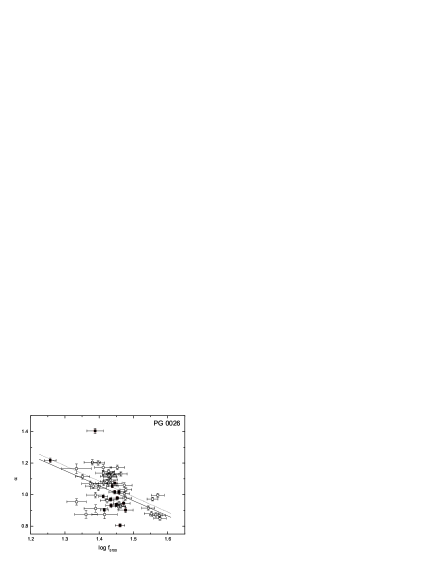
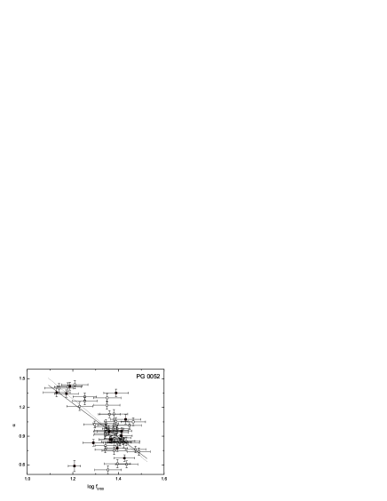
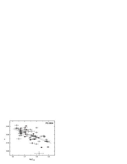
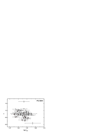
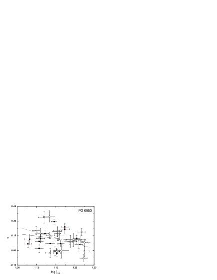
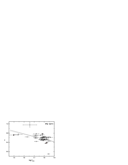
Figure 1: The spectral slope $\alpha$ versus the rest-frame 5100$\AA$ continuum flux $\log f_{5100}$ (in units of $10^{-16}ergs~{}s^{-1}cm^{-2}\AA^{-1}$) for each of these 17 PG QSOs. The spectral data from the Steward Observatory are solid rectangles, and the spectral data from the Wise Observatory are open rectangles, respectively. Solid lines are the best fit to all spectral data for each object while dotted lines are the best fit to the spectral data only from the Wise Observatory.

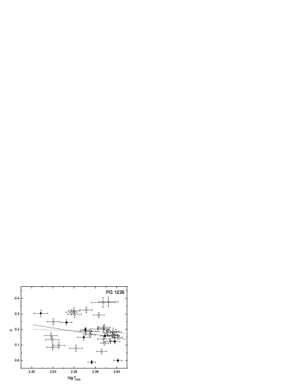
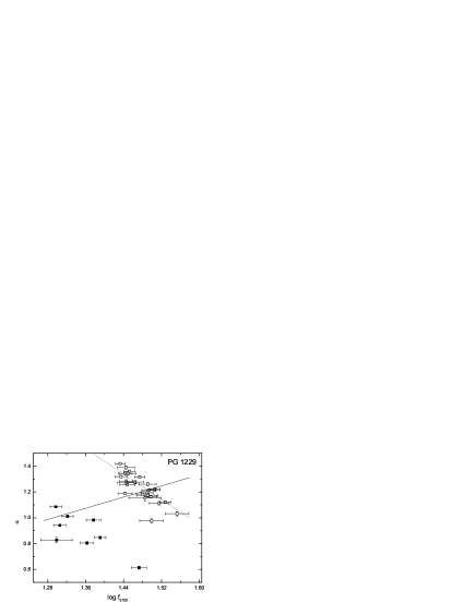
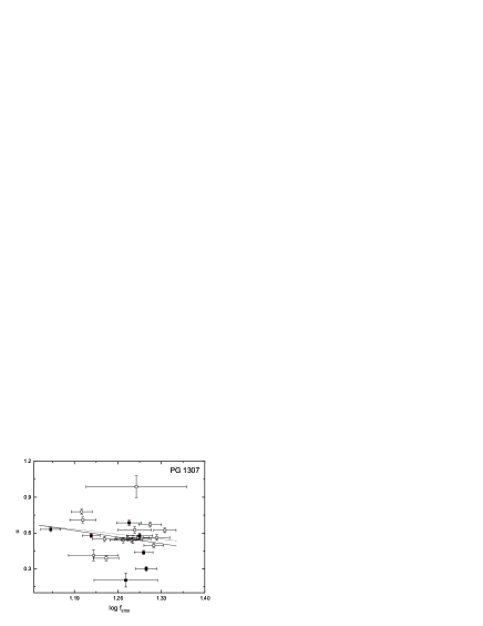
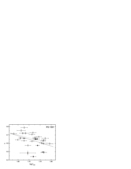
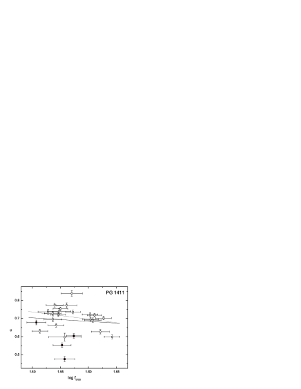
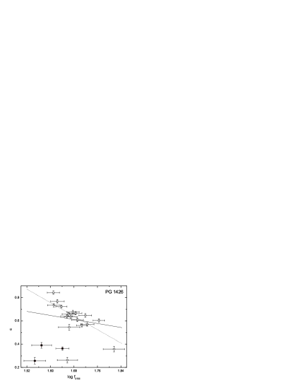
Figure 1: Continued.

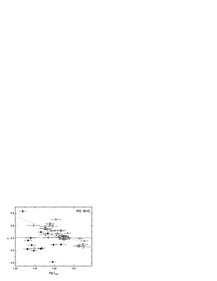
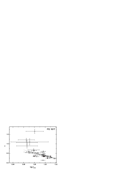
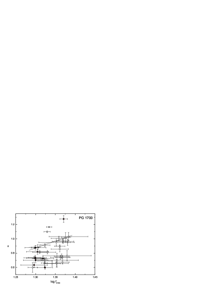
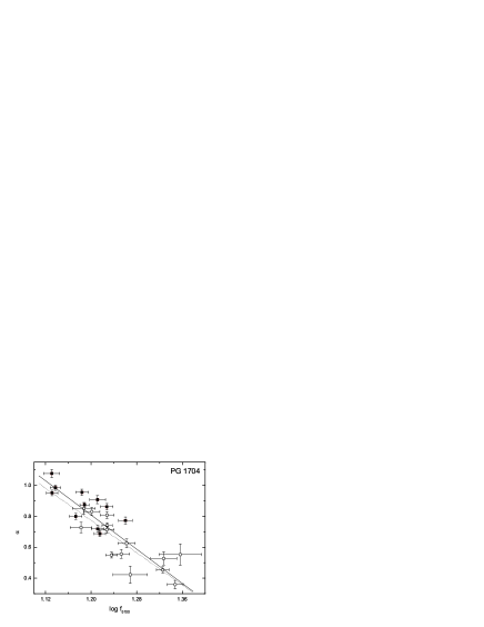
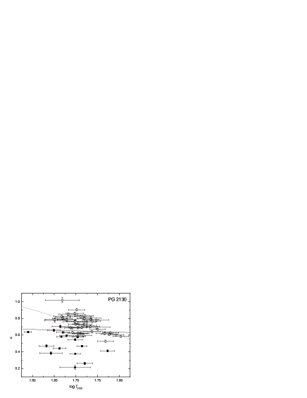
Figure 1: Continued.

In Fig. 1, we showed the spectral slope $\alpha$ as a function of the rest-frame 5100$\AA$ continuum flux $\log f_{5100}$ for each object. Considering the errors, it is obvious that all of these 17 PG QSOs exhibit spectral slope variability. We used the simple least-squares linear regression (Press et al. 1992) to study the correlation per object. For each object, we obtained the correlation coefficients (R) and the probabilities (P) for rejecting the null hypothesis of no correlation. The fitting results for all spectral data per object are listed in Col. (7) and (8) in table 1. These best fittings are also plotted in each panel (Fig. 1, solid lines). From Fig. 1 and table 1, we found that most of the objects showed negative correlation coefficients. Among the 15 QSOs which showed negative correlations, five objects PG 0026+129, PG 0052+251, PG 0804+761, PG 1617+175, and PG 1704+608 showed strong anti-correlations with $R>0.5$. Two objects, PG 1229+204 and PG 1700+518, existed moderate opposite trends. One radio-loud QSO, PG 1704+608, showed the strongest anti-correlation with $R=-0.88$. While the other radio-loud QSO, PG 1226+023 (3C 273), showed weaker anti-correlation with $R=-0.23$.

In order to give the ensemble relation for these 17 PG QSOs between the spectral slope and the luminosity, in the left panel in Fig. 2, we showed the average spectral slope $\alpha$ as a function of the average rest-frame 5100$\AA$ luminosity $\log L_{5100}$. We found that there existed a strong anti-correlation (R=-0.57, P=0.016). A simple least-squares linear regression gives the relation,

$$\alpha=(-0.38\pm 0.07)\log L_{5100}+(11.97\pm 2.08)$$ (1)

The best fitting is showed as solid line in Fig. 2. We also calculated the average Eddington ratio for each object, $L_{bol}/L_{Edd}$. The bolometric luminosity $L_{bol}$ is from luminosity in rest-frame 5100$\AA$: $L_{bol}=9\lambda L_{\lambda}(5100\AA)$, and $\rm L_{Edd}=1.26\times 10^{38}M_{BH}/\mbox{\,$\rm M_{\odot}$}~{}ergs~{}s^{-1}$, where the black hole mass is from Kaspi et al. (2000). In the right panel of Fig. 2, we plotted average $\alpha$ versus average Eddington ratio for each object. We found no correlation between them (R=0.064, P=0.081).

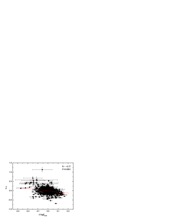
Figure 3: The spectral slope changes $\delta\alpha$ versus the rest-frame 5100$\AA$ continuum flux variations $\delta\log f_{5100}$. The solid line is our best fit.

Using the fitting slope of these 17 PG QSOs at all epochs, we correlated the spectral slope changes with the continuum flux variations. The changes of the spectral slope are calculated for each object between the slope of each observing date and the average spectral slope. In Fig. 3, the overall $\delta\alpha$ versus $\delta\log f_{5100}$ is plotted. We found an anti-correlation between the spectral slope changes and the continuum flux variations with $R=-0.27$ and $P<10^{-4}$. A simple least-squares linear regression gives,

$$\delta\alpha=(-0.61\pm 0.01)\times\delta\log f_{5100}-(5.91\pm 0.52)\times 10^{-3}$$ (2)

The best fitting is showed as the solid line in Fig. 3.

4 DISCUSSIONS AND RESULTS

These 17 PG QSOs data span 7.5 years with more than 20 epochs and are used in the reverberation mapping method to determine their central supermassive black hole masses (e.g. Peterson 1993; Kaspi et la. 2000). The time-span is enough to determine the variability of the optical spectral slope if any. For these high-luminosity PG QSOs, the contribution from the host galaxies is negligible. Here we used a power law function to fit data in the continuum bands suggested by kaspi et al. (2000). And then we obtained the spectral slope and the flux $f_{5100}$ in the rest-frame. Their errors are from our fitting. The results would possibly depend on the selection of the continuum bands. In order to be consistent with the continuum analysis of Kapsi et al. (2000), We adopted continuum bands suggested by kaspi et al. (2000) instead of usual continuum windows (Forster et al. 2001, Vanden Berk et al. 2001). In the future we will use the multi-component fitting method to avoid the selection effect of the continuum windows (Bian, Yuan & Zhao 2005).

4.1 Correlation for individual objects

Giallongo et al.(1991) investigated the long-term optical variability of quasars from photometric observations and found a positive correlation between variability and redshift. That QSOs at higher redshifts show larger variability since they are observed at a higher rest-frame frequency where the variability is stronger was indicated. This suggests a hardening in the bright phase of quasars. Statistical evidence for this trend were presented by follow-up studies (e.g. Cristiani et al. 1996, Di Clemente et al. 1996). Giveon et al.(1999) presented results from 7 yr photometric monitoring program of a well-defined, optically selected sample of 42 PG QSOs. The spectra of about half of the QSOs in their sample became harder when they brighten. The 42 objects in the optical sample included all 17 objects discussed in the present paper. Here on the basis of 7.5-year spectroscopic monitoring data of these 17 PG QSOs, we correlated the spectral slope with the rest-frame 5100$\AA$ continuum flux. The results showed that, among these 17 PG QSOs, five objects displayed strong anti-correlation with $R>0.5$ and there are nine objects with $R>0.3$ (See Fig. 1 and table 1). The anti-correlation implied that QSOs become bluer as they brighten. At the same time, other objects showed weaker correlation between $\alpha$ and $f_{5100}$ (See Fig. 1 and table 1). For PG 1700+518 and PG 1229+204, the correlation is possibly positive. The Fe II multiples are strong in PG 1700+518 (see Fig. 1 in Kaspi 2000). The strong Fe II emission may contaminate the selected continuum bands and the studying of the spectral slope variability for this object is probably influenced. The spectra of these 17 PG QSOs are from 2.3 m telescope at Steward Observatory and 1 m telescope at Wise Observatory. For each object, a large fraction of the spectral data are from the Wise Observatory. Considering only the spectra from the WO, a strong anti-correlation between the spectral slope and the continuum flux is found in PG 1229+204 ($R=-0.80$, $P<10^{-4}$) (see Fig. 1). The least-squares linear fitting using the spectral data only from the WO are also showed for all the other PG QSOs in our sample (Fig. 1, dotted lines). The result for this fitting are listed in Col. (9) and (10) in table 1. Using the spectra only from the WO, all but the object PG 1700+518 showed anti-correlation between the spectral slope and the continuum flux. Stronger anti-correlation are obtained for some of the objects (e.g. PG 1426+015, PG 1613+658, PG 2130+099).

4.2 Correlation for the ensemble of 17 objects

In order to clarify the slope variability, some authors discussed the relation between the spectral energy distribution (SED) changes and the continuum flux variations. Using the variation between two epochs in the photographic U, B_J, F, and N bands, Trevese et al.(2001) correlated the spectral slope changes $\Delta\alpha$ with brightness variations $\Delta\log f_{J}$ for a complete magnitude-limited sample of faint quasars in SA 57 and detected an average increase of the spectral slope (note that their $\alpha$ is defined by $f_{\nu}\propto\nu^{\alpha}$) for increasing continuum flux, indicating hardening of the spectrum in the bright phases. Trevese et al.(2002) performed an analysis of B and R observing data of 42 PG quasars from Giveon et al.(1999). They showed in their results that the average spectral slope of each QSO tended to be larger for brighter objects (the $\alpha$ is defined by $f_{\nu}\propto\nu^{\alpha}$). Using 7.5-year spectroscopic observing data, we discussed the relation between $\Delta\alpha$ and $\Delta\log f_{5100}$ for the ensemble of these 17 PG QSOs, a median anti-correlation ($R=-0.27$, $P<10^{-4}$) between them is found (see Fig. 3), indicating a hardening of the spectrum during bright phases which is consistent with the result of Trevese et al.(2001). We also found a strong anti-correlation between the average spectral slope and the average rest-frame 5100$\AA$ luminosity (See the left panel in Fig. 2) which is qualitatively consistent with the inter-QSO result of Trevese et al. (2002).

4.3 Model behind optical spectral variability

The physical mechanisms behind the optical variability of AGNs is largely unknown. Some models have been proposed to explain the AGNs optical variability properties. Current models can be classified mainly into three groups: accretion disk instabilities, discrete-event or Poissonian processes, and gravitational microlensing (e.g. Hawkins 1996, Aretxaga et al. 1997, kawaguchi et al. 1998, Kong et al. 2004). The optical spectral variability can provide clues to disentangle these models. Using the optical spectra of NGC 5548 between 1989 and 2001, Kong et al.(2004) found a strong correlation between $\alpha$ and the luminosity at rest-frame 5100$\AA$. They used the global variance of the accretion rates or/and the variance of the inner radius of the accretion disk to account for the strong relation. It can explain well the anti-correlation between the optical spectral index and the continuum luminosity observed in NGC 5548. Here in our PG QSOs sample, this disk instability model can also explain the anti-correlation which most of the objects showed between the spectral slope $\alpha$ and the rest-frame 5100$\AA$ continuum flux for individual QSOs. However, for the ensemble of our PG QSOs sample, the global variance of the accretion rates would not necessarily account for the global slope variance (See the right panel in Fig. 2). Vanden Beck et al. (2004) studied the ensemble photometric variability for about 25000 SDSS QSOs, that quasars are systematically bluer when brighter at all redshifts were found. Their result also seemed to disfavor gravitational microlensing and generic Poissonian processes as the primary source of quasar variability. QSOs are widely believed to be powered by the accretion disk onto a supermassive black hole (e.g. Rees 1984). It is natural to consider that the QSOs variability is due to some mechanisms associated with changes in the accretion processes. Kawaguchi et al. (1998) presented a very simple cellular-automaton model for disk instability. They gave the slope of structure function between 0.41 to 0.49, which is inconsistent with SDSS results (Vanden Beck et al. 2004). It is likely due to the complexity of possible accretion disk (or jet) instability models, which prevented more quantitative predictions.

5 Conclusion

Using 7.5-year spectroscopic monitoring data of a sample of 17 PG QSOs, we study the optical spectral slope variance. The main conclusions can be summarized as follows:

• Using the continuum bands suggested by Kaspi et al. (2000), we found that, in 7.5-years long-term observation, all 17 PG QSOs showed obvious optical spectral slope variability.

• Most of these 17 PG QSOs showed anti-correlation between the spectral slope $\alpha$ and the rest-frame 5100$\AA$ continuum flux $\log f_{5100}$ while five of them showed strong anti-correlation between $\alpha$ and $\log f_{5100}$ ($R>0.5$).

• For the ensemble of these 17 PG QSOs, a strong anti-correlation ($R=-0.57$) between the average spectral slope $\alpha$ and the average rest-frame 5100$\AA$ luminosity $\log L_{5100}$ is found while a median anti-correlation ($R=-0.27$) is found between spectral slope changes $\delta\alpha$ and continuum flux variations $\delta\log f_{5100}$ indicating a hardening of the spectrum during bright phases.

• The disk instability model can qualitatively explain the anti-correlation between the spectral slope $\alpha$ and the continuum flux $\log f_{5100}$ for individual QSOs. However, the global variance of the accretion rates would not necessarily account for the global slope variance for the ensemble of our PG QSOs sample. Accretion disk (jet) instability models with other mechanisms associated with changes in the accretion processes are promising.

Table 1: Sample properties. Col. 1:The name, Col. 2: redshift, Col. 3: apparent B magnitude, Col. 4: number of spectrophotometric observing epochs, Col. 5: the average optical spectral slope, Col. 6: average continuum flux density at rest wavelength 5100$\AA$ in units of $10^{-16}ergs~{}s^{-1}cm^{-2}\AA^{-1}$, Col. 7-8: correlation coefficient and probability for all spectra per object, Col. 9-10: correlation coefficient and probability for the spectra only from the Wise Observatory.

Object	z	$m_{B}$	N	$\alpha$	$f_{\lambda}$	R	P	$R_{Wise}$	$P_{Wise}$
(1)	(2)	(3)	(4)	(5)	(6)	(7)	(8)	(9)	(10)
PG 0026+129	0.142	15.3	56	$1.026\pm 0.116$	$27.4\pm 4.0$	-0.51	$<1\times 10^{-4}$	-0.62	$<1\times 10^{-4}$
PG 0052+251	0.155	14.7	56	$0.978\pm 0.229$	$22.4\pm 4.4$	-0.65	$<1\times 10^{-4}$	-0.70	$<1\times 10^{-4}$
PG 0804+761	0.100	14.5	70	$0.290\pm 0.097$	$55.7\pm 9.5$	-0.70	$<1\times 10^{-4}$	-0.69	$<1\times 10^{-4}$
PG 0844+349	0.064	15.1	49	$1.047\pm 0.157$	$37.8\pm 3.4$	-0.22	0.13	-0.38	0.024
PG 0953+414	0.239	15.4	36	$0.117\pm 0.101$	$15.7\pm 2.1$	-0.19	0.27	-0.42	0.046
PG 1211+143	0.085	14.4	38	$0.590\pm 0.177$	$58.1\pm 10.4$	-0.39	0.017	-0.35	0.050
PG 1226+023	0.158	12.8	39	$0.186\pm 0.091$	$218\pm 26$	-0.23	0.16	-0.083	0.66
PG 1229+204	0.064	15.5	33	$1.149\pm 0.189$	$27.9\pm 4.3$	0.38	0.028	-0.80	$<1\times 10^{-4}$
PG 1307+085	0.155	15.6	23	$0.564\pm 0.159$	$18.5\pm 2.0$	-0.34	0.12	-0.25	0.36
PG 1351+640	0.087	14.7	30	$0.637\pm 0.081$	$52.0\pm 5.0$	-0.49	$5.7\times 10^{-3}$	-0.52	0.010
PG 1411+442	0.089	15.0	24	$0.685\pm 0.080$	$36.8\pm 3.1$	-0.10	0.63	-0.29	0.22
PG 1426+015	0.086	15.7	20	$0.575\pm 0.166$	$46.3\pm 6.7$	-0.17	0.49	-0.65	$4.5\times 10^{-3}$
PG 1613+658	0.129	14.9	48	$0.423\pm 0.149$	$34.5\pm 4.4$	$-4.9\times 10^{-3}$	0.97	-0.74	$<1\times 10^{-4}$
PG 1617+175	0.114	15.5	35	$0.524\pm 0.316$	$13.8\pm 2.7$	-0.57	$3.4\times 10^{-4}$	-0.70	$<1\times 10^{-4}$
PG 1700+518	0.292	15.4	39	$0.828\pm 0.160$	$21.6\pm 1.5$	0.27	0.10	0.20	0.29
PG 1704+608	0.371	15.6	25	$0.733\pm 0.188$	$16.9\pm 2.4$	-0.88	$<1\times 10^{-4}$	-0.85	$1.1\times 10^{-4}$
PG 2130+099	0.061	14.7	64	$0.673\pm 0.150$	$50.6\pm 4.7$	-0.049	0.70	-0.57	$<1\times 10^{-4}$

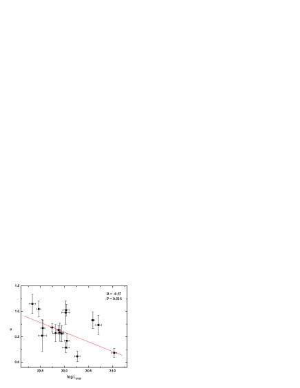
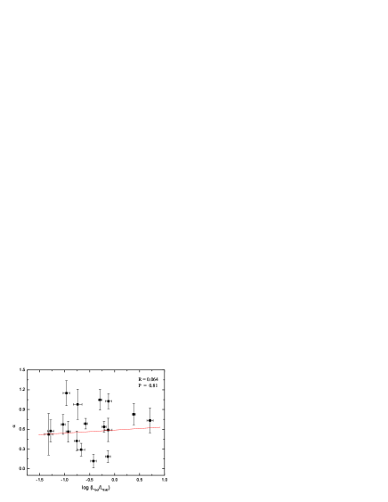
Figure 2: Left: the average spectral slope $\alpha$ versus the average rest-frame 5100$\AA$ luminosity $\log L_{5100}$ in units of $ergs~{}s^{-1}Hz^{-1}$ for 17 PG QSOs. Right: the average spectral slope $\alpha$ versus the average Eddington ratio for 17 PG QSOs. The solid lines are our best fits. The correlation coefficient R and the probability for rejecting the null hypothesis of no correlation are showed in the right figure corners.

References

- [] Aretxaga I., Cid Fernandes R., Terlevich R. J., 1997, MNRAS, 286, 271
- [] Bian W., Zhao Y., 2003, MNRAS, 343, 164
- [] Bian W., Yuan Q., Zhao Y., 2005, MNRAS, 364, 187
- [] Cid Fernandes R., Aretxaga I., Terlevich R., 1996, MNRAS, 282, 1191
- [] Cimatti A., Zamorani G., Marano, B., 1993, MNRAS, 263, 236
- [] Cristiani S., Trentini S., La Franca F. et al., 1996, A&A, 306, 395
- [] de Vries W. H., Becker R. H., White R. L., 2003, AJ, 126, 1217
- [] Di Clemente A., Giallongo E., Natali G. et al., 1996, ApJ, 463, 466
- [] Fan J. H., Lin R. G., 2000, ApJ, 537, 101
- [] Forster K., Green P.J., Aldcroft T.L. et al., 2001, ApJS, 134, 35
- [] Giallongo E., Trevese D., Vagnetti F., 1991, ApJ, 377, 345
- [] Giveon U., Maoz D., Kaspi S. et al., 1999, MNRAS, 306, 637
- [] Hawkins M. R. S., 1996, MNRAS, 278, 787
- [] Helfand D. J., Stone R. P. S., Willman B. et al., 2001, AJ, 121, 1872
- [] Huang K., Mitchell K. J., Usher P. D., 1990, ApJ, 362, 33
- [] Hook I. M., McMahon R. G., Boyle B. J. et al., 1994, MNRAS, 268, 305
- [] Kaspi S., Smith P. S., Maoz D. et al., 1996, ApJ, 471, L75
- [] Hawkins M. R. S. 1996, MNRAS, 278, 787
- [] Kawaguchi T., Mineshige S., Umemura M. et al., 1998, ApJ 504, 671
- [] Kaspi S., Smith P. S., Netzer H. et al., 2000, ApJ, 533, 631
- [] Kong M. Z., Wu X. B., Han J. L. et al., 2004, ChJaa, 4, 518
- [] Maoz D., Smith P. S., Jannuzi B. T. et al., 1994, ApJ, 421, 34
- [] Mushotzky R. F., Done C., Pounds K. A., 1993, ARA&A, 31, 717
- [] Nelson C. H., 2000, ApJ, 544, L91
- [] Peterson B. M., 1993, PASP, 150, 247
- [] Peterson B. M., 1993, PASP, 105, 247
- [] Rees M. J., 1984, ARA&A, 22, 471
- [] Press W. H., Teukolsky S. A., Vetterling W. T., Flannery B. P. 1992, Numerical Recipes, 2nd edition (Cambrigde: Cambridge Univ. Press)
- [] Shang Z. H. et al., 2005, 619, 41
- [] Trevese D., Kron R. G., Majewski S. R. et al., 1994, ApJ 433, 494
- [] Torricelli-Ciamponi G., Foellmi C., Courvoisier T. J.-L. et al., 2000, A&A, 358, 57
- [] Trevese D., Kron R. G., Bunone A., 2001, ApJ, 551, 103
- [] Trevese D., Vagnetti F., 2002, ApJ, 564, 624
- [] Vagnetti F., Trevese D., Nesci R., 2003, ApJ, 590, 123
- [] Vanden Berk D.E., Richards G.T., Bauer A. et al., 2001, AJ, 122, 549
- [] Vanden Berk D. E., Wilhite B. C., Kron R. G. et al., 2004, ApJ, 601, 692
- [] Wilhite B. C., Vanden Berk D. E., Kron R. G. et al., 2005, ApJ, 633, 638