Cosmic evolution of mass accretion rate and metalicity in
active galactic nuclei

Abstract

We present line and continuum measurements for 9818 SDSS type-I active galactic nuclei (AGNs) with $z\leq 0.75$. The data are used to study the four dimensional space of black hole mass, normalized accretion rate ($L/L_{Edd}$), metalicity and redshift. The main results are: 1. $L/L_{Edd}$ is smaller for larger mass black holes at all redshifts. 2. For a given black hole mass, $L/L_{Edd}$$\propto z^{\gamma}$ or $(1+z)^{\delta}$ where the slope $\gamma$ increases with black hole mass. The mean slope is similar to the star formation rate slope over the same redshift interval. 3. The FeII/H$\beta$ line ratio is significantly correlated with $L/L_{Edd}$. It also shows a weaker negative dependence on redshift. Combined with the known dependence of metalicity on accretion rate, we suggest that the FeII/H$\beta$ line ratio is a metalicity indicator. 4. Given the measured accretion rates, the growth times of most AGNs exceed the age of the universe. This suggests past episodes of faster growth for all those sources. Combined with the FeII/H$\beta$ result, we conclude that the broad emission lines metalicity goes through cycles and is not a monotonously decreasing function of redshift. 5. FWHM([O iii] $\lambda 5007$) is a poor proxy of $\sigma_{*}$ especially for high $L/L_{Edd}$. 6. We define a group of narrow line type-I AGNs (NLAGN1s) by their luminosity (or mass) dependent H$\beta$ line width. Such objects have $L/L_{Edd}$$\geq 0.25$ and they comprise 8% of the type-I population. Other interesting results include negative Baldwin relationships for EW(H$\beta$) and EW(FeII) and a relative increase of the red part of the H$\beta$ line with luminosity.

1. Introduction

Recent progress in reverberation mapping of type-I (broad emission lines) active galactic nuclei (AGNs) provide a reliable method for deriving the size of the broad line region (BLR) as a function of the optical continuum luminosity, the H$\beta$ line luminosity, the ultraviolet continuum luminosity and the X-ray (2–10 keV) luminosity (Kaspi et al. 2005, hereafter K05 and references therein). This has been used in numerous papers to obtain a “single epoch” estimate of the black hole (BH) mass by combining the derived BLR size with a measure of the gas velocity obtained from emission line widths, e.g. FWHM(H$\beta$) (e.g. Netzer 2003; Vestergaard 2004; Shemmer et al. 2004, hereafter S04; Baskin and Laor 2005). There are obvious limitations to such methods due to the scatter in the BLR size, the source luminosity and line width. These translate to a factor of 2–3 uncertainty on the derived masses when using the H$\beta$ line width as the velocity measure and the optical continuum luminosity ($\lambda L_{\lambda}$ at 5100Å, hereafter L₅₁₀₀) for estimating the BLR size. The uncertainty is larger, and perhaps systematic, when other emission lines are used. Additional uncertainties are associated with the currently limited luminosity range, $10^{42}\leq$L₅₁₀₀$\leq 10^{46}$ erg s^-1, thus mass determination for very luminous sources must be based on extrapolation. Notwithstanding the uncertainties, such methods can provide BH mass and accretion rate in large AGN samples that cannot be obtained in any other way.

This paper follows several earlier studies of type-I AGNs in the Sloan Digital Sky Survey (SDSS; see York et al. 2000) spectroscopic archive. The main aims are to obtain BH masses and accretion rates for a large number of such sources and to understand the time evolution and the metal content of the BLR gas. Earlier studies of this type include, among others, McLure and Jarvis (2002) and McLure and Dunlope (2004). Here we use the latest SDSS public data archive and a much larger number of sources compared with earlier studies. This enables us to obtain statistically significant correlations for various sub-samples of the data. We also introduce new, more robust methods for measuring the emission lines thus enabling more reliable study of metalicity and accretion rate.

This paper is organized as follows. In §2 we introduce our sample and explain the method of analysis and the various measurements performed on the SDSS spectra. In §3 we show the more important correlations pertaining to type-I sources and in §4 we give a discussion of the main results, including the derived redshift dependent accretion rate which we compare with the known star formation rate over the same redshift interval.

2. Basic measurements

2.1. Sample selection

The present sample contains all broad line AGNs in the SDSS sample from data release 4 (DR4, see Adelman-McCarthy et al. 2006 and references therein) with a redshift cut at $z=0.75$. This more than doubles the number of such sources in DR3 (Schneieder et al. 2005). The sources are defined as QSOs by the target selection algorithm but will be addressed here as type-I AGNs. The limit of 0.75 is dictated by the wavelength band of the SDSS spectroscopy and is designed to allow the measurement of the H$\beta$ and [O iii] $\lambda 5007$ lines and the 5100Å continuum in all sources. The inclusion of [O iii] $\lambda 5007$ is required for different line velocities and for omitting very few sources with such weak broad lines that they are confused with type-II AGNs. The requirement on H$\beta$ is motivated by the work of Kaspi et al. (2000) and K05 which present the only available reverberation mapping sample. This low redshift sample includes H$\beta$ and L₅₁₀₀ measurements for 35 sources and much fewer UV line and continuum measurements. The BLR size is obtained from the measured H$\beta$ lag (or a combination of $H\alpha$ and H$\beta$ lags) and the velocity from the observed FWHM(H$\beta$). Different lines have been used in several other papers (e.g. Vestergaard 2004; Vestergaard and Peterson 2006) yet their use is more problematic since it requires a secondary calibration against H$\beta$ and L₅₁₀₀. Of the two UV lines most commonly used, Mg ii $\lambda 2798$ is probably more reliable (e.g. McLure and Jarvis 2002; McLure and Dunlop 2004) and C iv $\lambda 1549$ suffers from various systematic effects (Baskin and Laor 2005 and references therein). We limit the present study to the use of H$\beta$ and defer the study of higher redshift AGNs, based on the Mg ii $\lambda 2798$ line, to a later publication.

The SDSS archive (Stoughton et al. 2002) was queried for QSOs with $z\leq 0.75$. This returned 14554 objects out of which 1212 were found to have problematic mask data (spectra with more than 30% flagged pixels; see Stoughton et al. table 11 for details). These objects are not included in the analysis. We decided to stick with the original magnitude limit of the sample at the time of target selection. This means that QSOs which are fainter than $i(mag)$=19.1 in the TARGET database, but were later added to the BEST database due to improved photometry, or objects that were added to the QSO database after their spectra were examined as different science targets (thus listed as ${\rm TARGET\_QSO\_FAINT}$ by the SDSS target selection algorithm; see §4.8.4 and table 27 in Stoughton et al.) were not included. This removes 1927 additional sources from the sample leaving 11415 sources with $i(mag)\leq 19.1$.

The spectra of all sources were corrected for Galactic extinction using the dust maps of Schlegel et al. (1998) and the Cardelli et al. (1989) model. Next, pixels with problematic MASK values (as defined above) are replaced by local interpolation and the spectra are de-redshifted and put on a uniform wavelength scale of 1Å per pixel.

2.2. Line and continuum measurements

Our work make use of the SDSS spectra as obtained from the archive without any attempt to subtract the galaxy contribution. This introduces some uncertainties at the low luminosity end of the sample and is addressed below in those cases where we consider it to be important for the derived correlations. The general issue of stellar contribution to AGN spectra of various luminosities is discussed in Bentz et al. (2006).

The emission lines measured in this work are [O iii] $\lambda 5007$, H$\beta$ and the FeII line complex between the wavelengths of 4000 and 5300Å. We first fit a linear continuum between two continuum bands: 4430–4440Å and 5080–5120Å. This continuum is subtracted from the spectrum and a five Gaussian model is fitted to the profiles of the two [O iii] lines and H$\beta$. The [O iii]$\lambda\lambda 4959,5007$Å lines are forced to have their theoretical intensity ratio (3.0), the same FWHM and their known wavelengths. The H$\beta$ line is fitted with two broad Gaussians and a single narrow Gaussian with FWHM and wavelength that agree with the [O iii] lines to within 200 km s^-1. At this stage, the narrow H$\beta$ component is not allowed to exceed 0.7 the intensity of [O iii] $\lambda 5007$. The broad H$\beta$ Gaussians are limited to FWHM of 1500–5000 km s^-1 and a shift of up to 500 km s^-1 relative to [O iii] $\lambda 5007$. These first limits are necessary in order to avoid the inclusion of some neighboring FeII lines, mostly on the blue side of the H$\beta$ profile, and to properly model the broad H$\beta$ components.

The next step involves fitting and deblending of FeII lines. The Boroson & Green (1992; hereafter BG92) Fe II emission template was convolved with a single Gaussian, which has the same FWHM as the broad H$\beta$ from the previous fit. The resulting FeII model is fitted to the spectra over the region 4400–4650Å. This region was chosen to minimize the effect of contamination with H$\beta$, HeII$\lambda 4686$ and [O iii] $\lambda 5007$. Next we measure the contribution of the FeII lines to the previously defined continuum bands, subtract this and refit the continuum. The entire procedure is repeated and the newly defined FeII template is subtracted from the continuum-subtracted spectrum. This leaves us with a FeII-free spectrum.

The final stage involves, again, a five Gaussian fit to the [O iii] and H$\beta$ lines. At this stage we relax the conditions and allow a broader range of Gaussians (as narrow as the [O iii] $\lambda 5007$ line and as broad as 20,000 km s^-1), and a larger shift between the narrow H$\beta$ and [O iii] $\lambda 5007$ (450 km s^-1). The 20,000 km s^-1 limit is required since almost all cases exceeding this limit are found to show poor quality fits (see below). We also allow shifts of up to $\pm 1000$ km s^-1 between each of the two broad H$\beta$ components and the wavelength of the narrow H$\beta$ line. All line and continuum measurements used later in the statistical analysis are based on the final stage of the fit and the second FeII fit. We found this multi-stage method to be more robust, and less prone to fitting inaccuracies compared with a single-stage fit of all line and components.

Regarding FWHM([O iii] $\lambda 5007$), we use an “intrinsic” line width which is obtained by properly subtracting a uniform instrumental line width of FWHM=140 km s^-1. We have decided not to include in the fit the blue wing commonly observed in the line profile. This removes a potential complication due to blending with the broad H$\beta$ profile and is also in line with earlier measures of the line in type-I and type-II sources. As explained in Greene & Ho (2005), a single component [O iii] $\lambda 5007$ line is a good indicator of $\sigma_{*}$. This point is further discussed in §3.5. We do not include in the analysis the He ii $\lambda 4686$ line which is clearly seen in many of the sources.

As for the broad H$\beta$ line, we measure its rest equivalent width (EW(H$\beta$)) and FWHM(H$\beta$) and also divide the combined line profile into two parts, at the rest wavelength of 4862Å (as determined by the wavelength of [O iii] $\lambda 5007$). The line flux is then measured in each part. We note that some earlier works followed BG92 and use EW(FeII) as a replacement for the iron line intensities. Here we define L(FeII) by integrating the line flux over the wavelength range of 4434–4684Å (e.g. S04). In what follows FeII/H$\beta$ stands for L(FeII)/L(H$\beta$).

The automated procedure to measure line and continuum fluxes suffers from various problems and limitations, some that are difficult to cure. To allow better control of the fit results, we make use of the $R^{2}$ and $\chi^{2}$ statistics (both per degree of freedom). These are combined in various ways to reject sources that do not fall within the predefined limits of $R^{2}>0.2$ and $\chi^{2}<5$. A common problem is encountered in weak flux sources with very large FWHM(H$\beta$). In many of these cases, mostly those at small redshift, the stellar contribution to L₅₁₀₀ is of the same order as the non-stellar continuum. The poor signal-to-noise (S/N) in some of those makes it difficult to properly fit the low contrast H$\beta$ profile. A similar problem occurs with very broad low contrast FeII blends which can result in erroneous, very large FeII/H$\beta$. Such objects are usually found and rejected by their small value of $R^{2}$. Given the strong dependence of luminosity on redshift, it is not surprising that such problems are less common at higher redshifts. Thus, the fit quality at high redshift is usually better even in sources that have low S/N due to being close to the flux limit of the sample. Our rather conservative approach results in the rejection of about 13% of all sources due to poor fits. Relaxing those criteria to include about half of the rejected sources in the analysis change very little the conclusions of the paper.

Radio information is readily available from the SDSS archive that provides FIRST (First Images of the Radio Sky at Twenty centimeters) data for all sources (e.g. Richards et al. 2002; McLure and Jarvis 2004). This enables us to divide the sample into radio loud (RL) and radio quiet (RQ) AGNs. The final sample that it analyzed here includes 9818 sources out of which 812 are RL-AGNs. Its luminosity distribution as a function of redshift is shown in Fig.1.

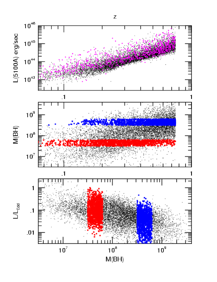
Figure 1.— Basic sample properties. Top panel: L₅₁₀₀ vs. redshift for RL (magenta points) and RQ (black points) type-I AGNs. Middle panel: M(BH) vs. redshift for type-I RQ-AGNs. Bottom panel: $L/L_{Edd}$ vs. M(BH) for type-I RQ-AGNs. Here and in all other diagrams, small black points mark the entire RQ sample while the colored dots represent sources in two mass groups: $10^{7.5-7.8}$ $M_{\odot}$ (red) and $10^{8.5-8.8}$ $M_{\odot}$ (blue).

2.3. Luminosity black hole mass and accretion rate

The combination of L₅₁₀₀ and FWHM(H$\beta$) was converted to BH mass using the most recent reverberation mapping results of K05. This gives

$$M(BH)=1.05\times 10^{8}\left[\frac{L_{5100}}{10^{46}\,{\rm erg\,sec^{-1}}}\right]^{0.65}\left[\frac{FWHM(H_{\beta})}{1000\,km/sec}\right]^{2}\,\,M_{\odot}\,.$$ (1)

The slope chosen here (0.65) is obtained from the R_BLR–L₅₁₀₀ relationship of K05. More recent papers (Vestergaard and Peterson 2006; Bentz et al. 2006) suggest a flatter slope (0.52) based on improved host galaxy subtraction in several of the low luminosity sources in the K05 sample, and the omission of several sources from the original list. We note that the inclusion of all the K05 sources in the Bentz et al. (2006) analysis, using the BCES method (see the Bentz et al. paper for explanation and their Table 1 for results) gives a slope of $0.57\pm 0.08$ which is entirely consistent with the K05 slope of $0.66\pm 0.07$. Moreover, there are other reasons for choosing a slope steeper than 0.52, e.g. using L(H$\beta$) as a proxy for the UV continuum luminosity (which is not affected by the host galaxy subtraction) gives such a slope. Finally, removing several of the faintest sources from the K05 sample also justifies this slope. For example, in 91% of the sources in our sample L₅₁₀₀$>10^{43.5}$ erg s^-1. Thus it is justified not to include the K05 sources with L₅₁₀₀$<10^{43.5}$ erg s^-1  when searching for the most suitable reverberation mapping relationship for the SDSS sample (this also avoids complications due to host galaxy contamination). This smaller sample produces a relationship very similar to the one given by eqn. 1.

The normalized accretion rate, $L/L_{Edd}$, is given by

$$L/L_{Edd}=\frac{f_{L}L_{5100}}{1.5\times 10^{38}[M(BH)/M_{\odot}]}\,\,,$$ (2)

where $f_{L}$ is the bolometric correction factor. Estimates of $f_{L}$ requires further assumptions about the spectral energy distribution (SED), in particular the luminosity of the unobserved, extreme UV continuum. This issue has been discussed in great detail in numerous publication. Estimates for $f_{L}$ in type-I AGN range between 5 and about 13 (e.g. Elvis et al. 1994; Kaspi et al. 2000; Netzer 2003; Marconi et al. 2004; S04). Excluding dust reprocessed radiation (that was included in the Elvis et al. 1994 SED), the range is about 5–10. There are clear indications from general considerations of the AGN luminosity function (Marconi et al. 2004), as well as from direct spectroscopy (e.g. Scott et al. 2004; Shang et al. 2005), that the shape of the SED is luminosity dependent and the ratio is larger in lower luminosity AGNs. Since the exact luminosity dependence is not known (see however Marconi et al. 2004, Fig. 3 for a specific suggestion) we adopt a constant ratio of $f_{L}=7$ which is roughly the mean between the value deduced for weak and strong UV bump sources. A more advance analysis can involve the actual Marconi et al. values. For the range of L₅₁₀₀ considered here (Fig. 1), this would cover the range $6.2<f_{L}<8.3$.

The rest of this paper includes various diagrams involving mass, luminosity and accretion rate of AGNs at different redshifts. Despite the specific expressions given in eqns. 1 and 2, none of those correlations is trivial since the dependence of luminosity on the BH mass is unknown a priori. Our work can be considered as a study of the four dimensional distribution of type-I AGNs along the coordinates of M(BH), $\dot{M}(BH)$, metalicity and redshift.

The SDSS is a flux limited sample and hence many of the derived correlations are affected by its redshift dependence incompleteness. In the following we take into account the flux limit of the sample which is transformed, as appropriate, to the various correlations under study. The limits on L₅₁₀₀, $L/L_{Edd}$ etc. are obtained from the (reddening corrected) $i(mag)$, the redshifts and a k-correction that assumes $L_{\nu}\propto\nu^{-0.5}$ across the wavelength range of interest (5100–8000Å).

Fig.1 shows BH mass as a function of redshift for all RQ-AGNs in our sample. It confirms the well known tendency for finding larger active black holes at higher redshifts, a result that was already presented by McLure & Dunlope (2004) over a wider redshift range. The lower boundary at each redshift is a clear manifestation of the strong correlation of M(BH) and L₅₁₀₀ in our flux limited sample. The diagram is very similar to the one presented in McLure & Dunlope (2004) where a smaller sample and somewhat different expressions for deriving M(BH) and $L/L_{Edd}$ have been used. Here, and in several other diagrams, we focus on two mass groups that are marked in two different colors: $10^{7.5-7.8}$ $M_{\odot}$ (red, 1207 sources) and $10^{8.5-8.8}$ $M_{\odot}$ (blue, 1422 sources).

McLure and Jarvis (2004) used a sample of about 6,000 SDSS QSOs to investigated the mass of the central BHs as a function of radio properties. They found that RL-QSOs host, on the average, more massive BH for a given optical continuum luminosity. The mean M(BH) difference between RL-AGNs and RQ-AGNs found by those authors is 0.16 dex. This was attributed to the larger mean FWHM(H$\beta$) in radio loud sources. We checked these findings by comparing the luminosity, BH mass and $L/L_{Edd}$ for the two populations in our $z\leq 0.75$ sample. Using the medians of all properties, we find a difference of 0.11 dex in L₅₁₀₀, a factor of 1.06 in FWHM(H$\beta$), and a difference of 0.15 dex in M(BH) (the differences in the mean are somewhat larger). The difference in M(BH) is, of course, the result of the differences in luminosity and line width between the two populations (see eq. 1).

Fig. 1 also shows $L/L_{Edd}$ vs. M(BH) for the RQ-AGN sample as well as for the two mass groups. The low accretion rate limit is determined, mostly, by the flux limit of the sample. Thus, we expect that more object with small $L/L_{Edd}$ are missing at higher redshifts. The highest accretion rate sources in each mass group are not affected by this limit. Based of these sources we confirms that the lowest mass BHs are the fastest accretors, a result that was already noted by McLure and Dunlop(2004).

3. Results

3.1. Accretion rate vs. redshift

The correlation of $L/L_{Edd}$ with redshift for the entire sample, as well as for the two mass groups, is shown Fig. 2. The diagram shows also two computed lower limits for each of the two groups corresponding to the flux limits of the two mass boundaries. The visual impression is somewhat misleading since much of the apparent correlation is due to the lower limit on $L/L_{Edd}$ resulting from the flux limits on the various mass groups. The presence of such flux limits considerably complicate the analysis and we have searched for rigorous ways to derived the intrinsic z-$L/L_{Edd}$ dependence. Below we detail the two methods that were used, the peak of the $L/L_{Edd}$ distribution and the Efron and Petrosian (1992) truncated permutation test.

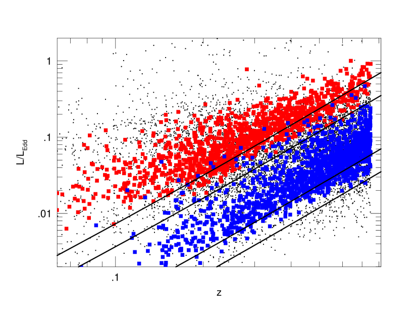
Figure 2.— $L/L_{Edd}$ vs. redshift for our SDSS sample of type-I RQ-AGNs. The solid lines represent the limiting accretion rates obtained from the flux limits for the two mass groups (see text). Symbols are the same as those of Fig.1.

3.1.1 The peak distribution method

We first study the distribution of $L/L_{Edd}$ in several redshifts bins that are just wide enough to include a reasonable number of sources. These histograms (see Fig. 3) are used to define the peak and the envelope of the $L/L_{Edd}$ vs. redshift relationship. The bins are defined such that $\Delta z/z=0.1$ and include from 50 to 230 sources, with an average number of about 120 sources per bin.

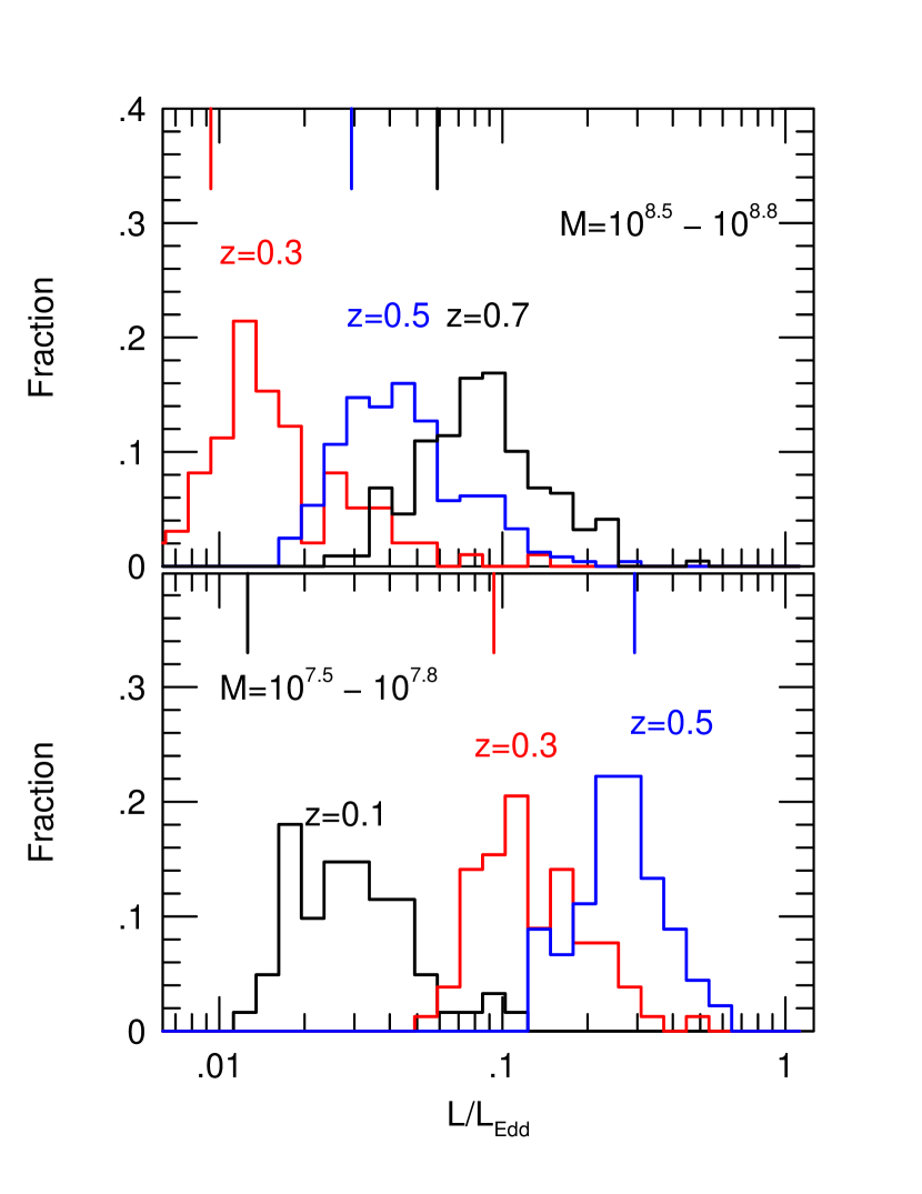
Figure 3.— $L/L_{Edd}$ histograms for various redshift bands, as marked, for the low (bottom) and high (top) mass groups. The redshift bins are defined in the text. The vertical lines at the top of each panel mark the conservative lower limit on $L/L_{Edd}$ obtained from the flux limit of the same color histogram (see text for more details).

Such a procedure is only meaningful if the peak of the distribution is clearly defined, i.e. if the value of $L/L_{Edd}$ corresponding to the maximum number of sources is larger than the accretion rate imposed by the flux limits of the sample. There are four such limits for each bin: two corresponding to the redshift boundaries and two to the mass boundaries. The largest of those four (i.e. the most conservative limits) are shown in Fig. 3 for each of the two mass groups and several redshift bins. As evident from the diagram, the peaks of the $L/L_{Edd}$ distribution in the lower mass group (bottom part of the diagram) are only meaningful for $z\leq 0.3$. Beyond this redshift the method is not applicable since the SDSS survey is not deep enough to properly sample many sources and the limiting $L/L_{Edd}$ is larger than the value at the peak. The larger mass group (top panel) is less problematic and the histograms show that the peaks are well defined for $0.3\leq z\leq 0.75$. The z=0.2 histogram (not shown here) can also be used to define the peak.

As an independent check on the slope of the correlation in those redshift intervals where the peak distribution can be identified, we also used the upper envelope of the distribution which we define by the fifth largest $L/L_{Edd}$ (the number of sources with larger $L/L_{Edd}$ is so small in some groups that we suspect incomplete sampling). Obviously, the upper envelop is not affected by the flux limit of the sample. However, the redshift bins must contain enough sources to justify this method. This may be a problem for very high luminosity sources at low redshift because of the limited area covered by the SDSS sample.

The results of the test are shown in Fig. 4. We also show the peaks of the distribution for a third mass group, with M$=10^{6.8-7.2}$ $M_{\odot}$, for those redshifts where the peak of the $L/L_{Edd}$  distribution is higher than the flux limit of this group. In this mass range, this is only true for $z<0.25$ since there are very few such low mass sources at higher redshifts because of the flux limit. The results can be presented as simple power-laws in redshift ranging from $L/L_{Edd}$$\propto z^{0.8}$ for for M(BH)=$10^{7}$ $M_{\odot}$ to about $L/L_{Edd}$$\propto z^{2.2}$ for M(BH)=$10^{8.6}$ $M_{\odot}$. Given the small number of points in the various redshift intervals, and the differences between the slopes obtained from the peaks and the envelopes of the various histograms, we estimate an uncertainty of about 0.3 on the slopes obtained with this method.

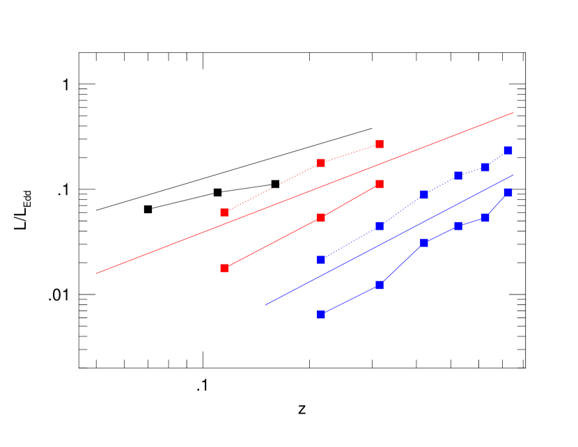
Figure 4.— $L/L_{Edd}$ vs. z for various mass groups. The color symbols correspond to the two mass groups where solid line represent peaks and dotted lines represent the upper envelopes of the distributions, as explained in the text. Black lines and symbols represent a third mass group with M=$10^{6.8-7.2}$ $M_{\odot}$. The straight solid lines are the results of the truncated permutation test for the same mass groups (eqn.4 and Table 1).

3.1.2 The truncated permutation test

The determination of bivariate distributions from truncated astronomical data is a well known problem. Such data sets are very common and the flux limited sample considered here is only one such example. The problem is to test such truncated bivariate data sets for statistical independence without a priori knowledge of the real underlying correlation. This issue is discussed in great detail by Efron & Petrosian (1992; see this paper for earlier attempts to address this issue) who suggest powerful nonparametric permutation tests that can be applied to data sets of this type. The paper describes tests for nontruncated as well as truncated data sets and apply them to two astronomical cases that are rather similar to the sample in question. In particular, they describe a rank-based statistics that is powerful, robust and easily administrated to data sets like ours.

The normalized rank statistic of Efron and Petrosian (1992), $T_{i}$, is used to define a test statistic

$$t_{w}(data)=\Sigma_{i}w_{i}T_{i}/(\Sigma_{i}w_{i}^{2})^{1/2}\,\,,$$ (3)

where w̌$=(w_{1},w_{2},....w_{n})$ is a vector of weights. $t_{w}(data)$ has mean 0 and variance 1 and is distributed normally thus allowing to obtain the best value and the confidence limits using the normal approximation (see Efron & Petrosian 1992 §3 for more details and definitions). The choice made here, and recommended also in Efron & Petrosian (1992), assumes equal weights for all points, i.e. w̌$=(1,1,....1)$. The application of the permutation test involves a guess of the real distribution which recovers the null hypothesis of independence between the two variables in questions (in our case $L/L_{Edd}$ and z).

We have used truncated permutation tests to check two families of ad hoc luminosity redshift dependences:

$$L/L_{Edd}\propto z^{\gamma(M)}\,\,,$$ (4)

and

$$L/L_{Edd}\propto(1+z)^{\delta(M)}\,\,.$$ (5)

This involved changing the guessed values of $\gamma$ and $\delta$, for various mass groups, and looking for their best values (i.e. those $\gamma$ and $\delta$ resulting in $t_{w}=0$) as well as the 90% confidence limits (those value giving $t_{w}=-1.645$ and $t_{w}=1.645$). The mass groups used were limited to be 0.2 dex wide except for the lowest mass group, around M(BH)=$10^{7}$ $M_{\odot}$, where the small number of objects dictates a wider range (0.4 dex). The results are listed in Table 1 where we also specify the redshift range for each group (the largest mass group contains no objects at small z and the lowest mass group contains very few sources at $z>0.25$ hence the need to define a redshift range).

The results of the test are shown in Fig. 4 for the case of eqn. 4. They are consistent with the results of the peak distribution method and lend support to the interpretation that the peak of the distribution has indeed been recovered for the mass groups and redshift intervals discussed above. These results are further discussed and compared with the cosmic star formation rate in §4.2

Table 1Fit coefficients for $L/L_{Edd}$ vs. $z$ (eqns. 4 & 5)

$\log M$ ($M_{\odot}$)	$\Delta z$	$\gamma$ (90% limits)	$\delta$ (90% limits)
7.0	0.05–0.3	1.02 (0.91–1.13)	8.6 (7.7–9.7)
7.5	0.05–0.75	1.25 (1.15–1.34)	7.6 (7.1–8.05)
8.0	0.1-0.75	1.61 (1.54-1.67)	6.8 (6.6–7.1)
8.5	0.20–0.75	1.79 (1.70–1.87)	6.1 (5.7–6.3)
9.0	0.25–0.75	2.30 (2.15–2.47)	7.6 (7.1–8.1))

3.2. FeII/H$\beta$ and iron abundance

Fig. 5 shows the dependence of FeII/H$\beta$ on $L/L_{Edd}$ for our sample of type-I SDSS AGNs. As clear from the diagram, and has been verified by standard regression analysis, FeII/H$\beta$ and $L/L_{Edd}$ are significantly correlated and larger $L/L_{Edd}$ are associated with stronger FeII and/or weaker H$\beta$ lines. This conclusion applies for all sources with $L/L_{Edd}$$\raisebox{-2.15277pt}{$\;\stackrel{{\scriptstyle>}}{{\sim}}\;$}0.03$ while at lower accretion rates the scatter is too large to see a definite trend. Such a correlation has been suspected in the past and has studied in several previous papers (see Netzer et al. 2004 and references therein). However, it was never tested in such a large sample and over the entire 0–0.75 redshift range.

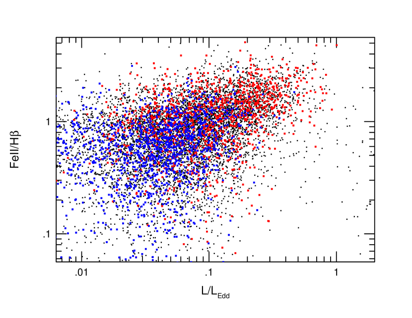
Figure 5.— FeII/H$\beta$ vs. $L/L_{Edd}$ for our SDSS sample of type-I RQ-AGNs. Symbols are the same as those of Fig.1.

We have also studied the dependence of FeII/H$\beta$ on redshift in the entire sample as well as in the various mass groups. Simple linear regression suggests that, for RQ-AGNs, FeII/H$\beta$$\propto z^{-0.22\pm 0.02}$. The slope is somewhat steeper for RL sources ($-0.38\pm 0.07)$ and for the mass group of $10^{7.7-7.8}$ $M_{\odot}$ objects ($-0.40\pm 0.05$). The large number of points in all those groups of sources results in formally significant correlations. However, detailed examination shows that the results depend strongly on the measured FeII/H$\beta$ at the low redshift low luminosity end of the distribution. As explained in §2.2, some of these cases, especially those with extremely broad lines, are difficult to measure and are therefore uncertain because of the large stellar contribution. There are indeed differences in the mean FeII/H$\beta$ between the $z<0.2$ and $z>0.5$ redshift bins but not a smooth continuous change as a function of redshift. In view of this, we consider the evidence for redshift dependence of FeII/H$\beta$ as marginal. This uncertainty does not affect the FeII/H$\beta$ vs. $L/L_{Edd}$ correlation discussed earlier.

The modeling of FeII line formation in AGN clouds is extremely complicated. It involves hundreds of energy levels and thousands of transitions. Earlier detailed studies by Netzer and Wills (1983) and Wills, Netzer & Wills (1985), that included most of the important atomic processes, reached the conclusion that the FeII line intensities are too uncertain to be used as iron abundance indicators. Major improvements in atomic data (Sigut & Pradhan 2003), combined with improved treatment of some of the line excitation processes (Baldwin et al. 2004), resulted in a better understanding of several strong FeII features but changed little with regard to the main conclusion: there are several mechanisms capable of enhancing FeII emission relative to the hydrogen Balmer lines and increased iron abundance is only one of them .

The correlation shown in Fig. 5 provides a new way to solve the iron abundance problem. As shown in S04, the N/C abundance (and metalicity in general) as measured from the N v $\lambda 1240$/C iv $\lambda 1549$ line ratio (Hamann et al. 2002 and references therein) is strongly correlated with $L/L_{Edd}$ over a large luminosity range. This result is in conflict with the earlier studies by Hamann and Ferland (1993; 1999) who suggested that the N/C ratio depends on source luminosity (see also Dietrich et al. 2002; Dietrich et al. 2003 for the possible dependence on M(BH)). The S04 finding is based mostly on the high metalicity of low luminosity narrow line Seyfert 1 galaxies (NLS1s) that do not fall on the original Hamann and Ferland (1993) correlation (Shemmer and Netzer 2002). The high metalicity of NLS1s gains further support by the detailed analysis of the absorption line spectrum of Mrk 1044 (Fields et al. 2005).

Given the dependence of metalicity on $L/L_{Edd}$, and the correlation of FeII/H$\beta$ with $L/L_{Edd}$ shown in Fig. 5, we suggest that FeII/H$\beta$ is an iron abundance indicator for all sources with $L/L_{Edd}$$\raisebox{-2.15277pt}{$\;\stackrel{{\scriptstyle>}}{{\sim}}\;$}0.03$. This conclusion does not rely on uncertain atomic models and complicated radiative transfer in photoionized BLR clouds. It is based on observed correlations in large AGN samples. There is no accurate way to calibrating the iron-to-hydrogen abundance because of the uncertain modeling. However, we can compare this relationship to the S04 correlation of N v $\lambda 1240$/C iv $\lambda 1549$ vs. $L/L_{Edd}$ (their Fig. 6). The comparison shows that the slopes of the two correlations are similar. For example, the use of the BCES method with the assumption of a uniform error of 0.1 dex in both axes gives FeII/H$\beta$$\propto$$L/L_{Edd}$^0.7. Assuming that Fe/H scales with O/H, and using the Hamann et al. (2002) calculation to calibrate N/C vs. metalicity, we find that solar Fe/H corresponds to FeII/H$\beta$$\simeq 0.6$.

3.3. The growth time of massive black holes

Next we assume that BH growth is dominated by gas accretion and BH mergers are of secondary importance. Given this assumption, we can calculate the growth time using the Salpeter (1964) original expression as

$$t_{\rm grow}=4\times 10^{8}\frac{\eta/(1-\eta)}{L/L_{Edd}}\log\frac{M}{M_{\rm seed}}\frac{1}{f_{\rm active}}\,\,{\rm yr}\,,$$ (6)

where $f_{\rm active}$ is the fraction of time the BH is active. For simplicity we assume a mass independent accretion efficiency of $\eta=0.2$, to reflect the assumption of a non-zero angular velocity BHs, and a relatively large seed BH mass of $M_{seed}=10^{4}$ $M_{\odot}$. Obviously there is a range in both properties (e.g. Heger and Woosley, 2002; Ohkubo et al. 2006) but the analysis is not very sensitive to either of those provided $M_{seed}$ is not much larger than assumed here.

Given the above growth time, and assuming, $f_{\rm active}=1$, we can calculate for each BH the time required to grow to its observed mass relative to the age of the universe at the observed redshift, $t_{grow}/t_{universe}$. This is shown in Fig. 6 for all sources as functions of both $L/L_{Edd}$ and redshift. Evidently, most (66%) BHs did not have enough time to grow to their measured mass given their observed accretion rate. The fraction of such sources found here is, of course, an upper limit, since all BHs missing from our sample, due to their very small $L/L_{Edd}$ and the SDSS flux limit, also belong in this group of objects. Given the assumption of growth by accretion, we find that in the majority of cases, there must have been one or more past episodes where the accretion rate was higher than the value measured here. As shown in §4 below, this conclusion is of major importance in understanding the time dependent metal enrichment in AGNs.

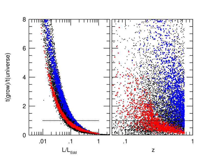
Figure 6.— BH growth-time, relative to the age of the universe, as a function of $L/L_{Edd}$ (left) and redshift (right). Objects above the horizontal line at t(grow)/t(universe)=1 must have had past episodes of faster accretion. Symbols are the same as those of Fig.1.

3.4. Redefining narrow line type-I AGNs (NLAGN1s)

The subgroup of NLS1s is usually assumed to contain AGNs with the largest accretion rates (e.g. Grupe et al. 2004 and references therein). Such sources were first discussed in Osterbrock and Pogge (1985) who introduced the defining criteria of FWHM(H$\beta$)$\leq 2000$ km s^-1. NLS1s are known to have other extreme properties such as extremely steep soft X-ray continuum and larger than average FeII/H$\beta$.

The recent study by S04 includes H and K-band spectroscopy of about 30 high redshift, very high luminosity AGNs. In most of these sources $L/L_{Edd}$$>0.4$ yet FWHM(H$\beta$) is much larger than 2000 km s^-1. These authors suggested that the defining criteria for NLS1s should be mass and luminosity dependent thus reflecting the fundamental physics affecting the line width. This approach is different from the one taken by McLure and Dunlop (2004) who assumed the boundary between the groups of narrow and broad line type-I AGNs is at 2000 km s^-1, independent of luminosity. Given this assumption, they did not find a larger fraction of NLS1s among the highest luminosity sources in their sample.

Our SDSS sample contains a large enough range in both M(BH) and $L/L_{Edd}$ to study the S04 suggestion in more detail. To illustrate this we plot in Fig. 7 accretion rates as a function of FWHM(H$\beta$) for all sources and shaw, on the same diagram, the two mass groups introduced earlier and 31 high redshift sources from S04. The median mass for the third group is about $3\times 10^{9}$ $M_{\odot}$ and the median L₅₁₀₀ about $10^{46.6}$ erg s^-1 (an orders of magnitude larger than the most luminous $z\leq 0.75$ SDSS sources). The diagram shows also a line at $L/L_{Edd}$=0.25 that intersects the various subgroups at different line widths. At small $z$, this line is consistent with the Osterbrock & Pogge (1985) definition of NLS1s in terms of continuum luminosity and BH mass. We suggest that this line is a more physical measure of a general group of “narrow line type-I AGN” (hereafter NLAGN1s). Using eqns. 1 and 2 with $f_{L}=7$, and normalizing the relationship to have a boundary at $L/L_{Edd}$=0.25, we get either a luminosity-based definition,

$$FWHM(H_{beta})\leq 1870\left[\frac{L_{5100}}{10^{44}\,{\rm erg\,s^{-1}}}\right]^{0.175}{\rm km\,s^{-1}}$$ (7)

or a definition based on black hole mass,

$$FWHM(H_{beta})\leq 1700\left[\frac{M}{10^{7}\,M_{\odot}}\right]^{0.175}{\rm km\,s^{-1}}\,.$$ (8)

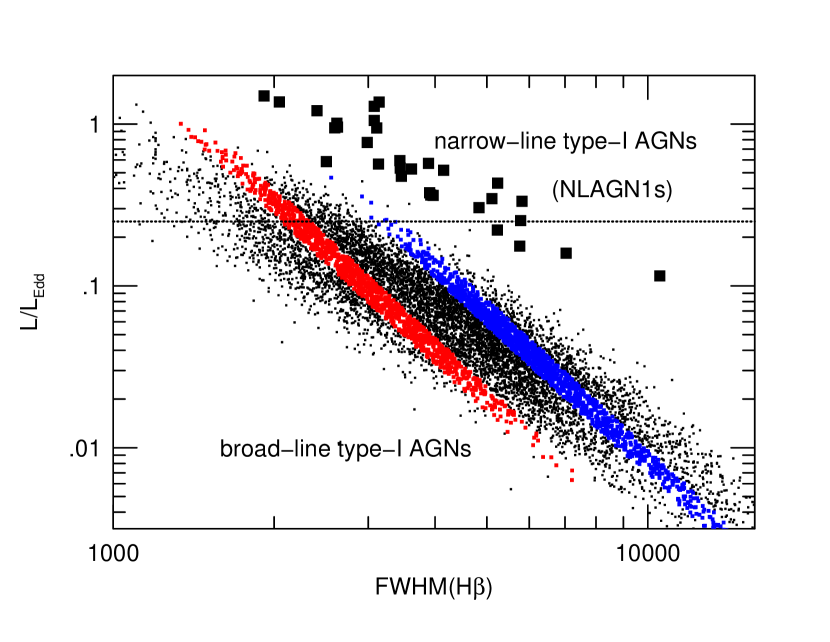
Figure 7.— A new definion of narrow line type-I RQ-AGN (NLAGN1s) based on accretion rate. The large symbols represent very luminous AGNs from S04 with a median BH mass of $10^{9.5}$ $M_{\odot}$. The dividing line is drawn at $L/L_{Edd}$=0.25. Symbols are the same as those of Fig.1.

3.5. FWHM([O iii] $\lambda 5007$) as a black hole mass indicator

The discovery of a tight correlation between black hole mass and the stellar bulge velocity dispersion ($\sigma_{*}$) resulted in several attempts to investigate secondary mass indicators related to emission line widths ($\sigma_{g}$). This is particularly important in those cases where the strong non-stellar continuum prevents the measurement of $\sigma_{*}$. For example, FWHM([O iii] $\lambda 5007$) has been suggested as a proxy for $\sigma_{*}$ in type-I AGNs (e.g. Nelson 2000; Shields et al. 2003; Grupe & Mathur 2004; Boroson 2003; Boroson 2005).

Boroson (2003) used a small subsample of 107 objects with $z<0.4$ from the early release SDSS data to study the FWHM([O iii] $\lambda 5007$) vs. $\sigma_{*}$ relationship. The FWHM([O iii] $\lambda 5007$) in this study was measured from the observed line profile with no profile fitting. He finds a real correlation between FWHM([O iii] $\lambda 5007$) and the BH mass with a flattening of the relationship at higher luminosity and a very large scatter (a factor of $\sim 5$). In a later publication, Boroson (2005) revisited the same problem using a larger sample (about 400 sources) covering the same redshift interval and focusing on the systemic velocity indicated by the [O iii] $\lambda 5007$ line center. He finds a systematic blueshift of the line peak with a magnitude which is correlated with the line width and with $L/L_{Edd}$. An extensive discussion of the merit of such techniques, including an analysis of a large sample (1749 object) of type-II AGNs, with a median redshift of 0.1, where both $\sigma_{*}$ and the width of several narrow emission lines have been measured, is given in Greene & Ho (2005). According to these authors, FWHM([O iii] $\lambda 5007$)/2.35 is a good proxy for $\sigma_{*}$ provided the strong line core, without the commonly observed extended blue wing, is used to define FWHM([O iii] $\lambda 5007$). Greene & Ho further suggested that deviations between $\sigma_{*}$ and FWHM([O iii] $\lambda 5007$)/2.35 are related to $L/L_{Edd}$. Large deviation probably reflect non-virial motions due to a strong radiation field. The [O iii] $\lambda 5007$ line luminosity has also been used as a primary bolometric luminosity indicator for type-II AGNs (e.g. Heckman et al. 2004) whose non-stellar continuum cannot be directly observed. As shown by Netzer et al. (2006), this is associated with a large scatter, and perhaps also a luminosity and/or redshift dependence.

Our SDSS sample is different from all earlier ones by being much larger and by covering a wider redshift range. It can thus be used to test the earlier findings regarding type-I AGNs at higher luminosities and redshifts and with a better statistics. Unlike Boroson (2003; 2005) and Greene & Ho (2005), we do not restrict ourselves to high S/N spectra and attempt to fit all sources with a detectable [O iii] $\lambda 5007$ line. As explained in §2.2, our FWHM([O iii] $\lambda 5007$) is based on a single Gaussian fit to the core of the line, similar to the method of Greene & Ho (2005). We have correlated these measurements with M(BH) and $L/L_{Edd}$ measured here and show the results in Fig 8 as M(BH) vs. FWHM([O iii] $\lambda 5007$) for the entire sample as well as for two redshift groups: z=0.1–0.2 and z=0.4–0.6. To guide the eye, we have calculated the best slope for each of the groups using the BCES method assuming a uniform error of 0.1 dex and plot them on the diagram together with a curve representing the Tremaine et al. (2002) parametrization of the M(BH)-$\sigma_{*}$ relationship.

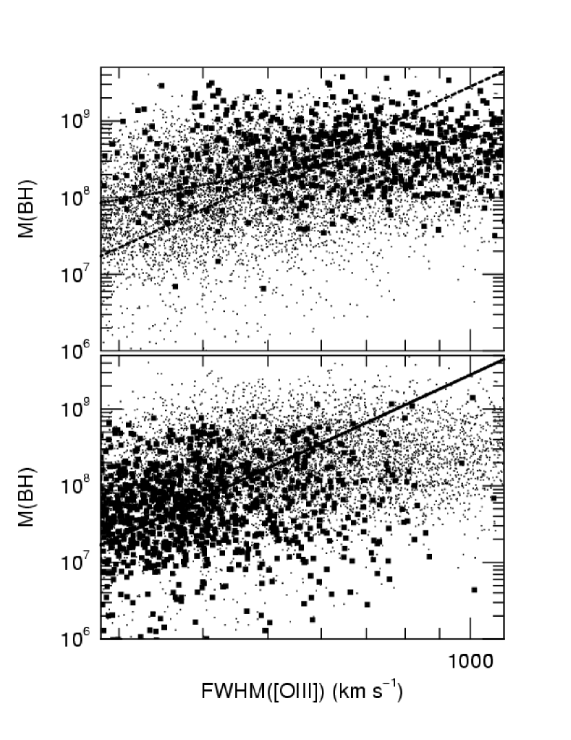
Figure 8.— The correlation of M(BH) vs. FWHM([O iii] $\lambda 5007$) for two redshift bins: z=0.1–0.2 (bottom) and z=0.4–0.6 (top). The entire RQ sample is plotted as small points in both panels and the objects belonging to the specific redshift group are plotted as large black symbols. The two lines in each panel are best fit curves for the redshift group in question (solid line) and the Tremaine et al. (2002) fit to the M(BH)-$\sigma_{*}$ relationship (dashed line). The two fits are basically identical for the z=0.1–0.2 group.

Fig. 8 clearly shows the non-linear dependence of log(M(BH)) on log(FWHM([O iii] $\lambda 5007$)). Expressing the correlation as M(BH)$\propto$FWHM([O iii] $\lambda 5007$)^α(z) we find a range of $\alpha(z)$ as listed in Table 2. As evident from the table, the slope is decreasing with redshift and the correlation becomes insignificant at $z>0.5$. As a curiosity, the agreement with the Tremaine et al. (2002) best slope ($\alpha=4.02$) is almost perfect over the redshift interval of 0.1–0.2 (see bottom panel of diagram). We suspect that the overall agreement between $\sigma_{*}$ and FWHM([O iii] $\lambda 5007$)/2.35 found by Grupe & Mathur (2004) and by Greene & HO (2005), is the result of those samples being dominated by low redshift sources.

Table 2Fit coefficients for M(BH) vs. FWHM([O iii] $\lambda 5007$) as defined in §3.5

$\Delta z$	$\alpha(z)$	$L/L_{Edd}$	$\beta(L/L_{Edd})$
0.05–0.15	$5.8\pm 1.5$	0.01–0.03	$3.4\pm 0.1$
0.10–0.20	$4.0\pm 0.6$	0.10–0.15	$2.7\pm 0.7$
0.37–0.43	$1.6\pm 0.2$	0.30–0.50	$2.1\pm 0.2$
0.66–0.75	$1.5\pm 0.9$	all	$2.9\pm 0.4$

High accretion rate can also influence the [O iii] $\lambda 5007$ line width by introducing a non-virial component to the line profile, perhaps due to acceleration by radiation pressure force. This has been studied by Netzer et al. (2004), Boroson (2005) and Greene & Ho (2005). Netzer et al. found that FWHM([O iii] $\lambda 5007$) correlates with L₅₁₀₀, M(BH) and $L/L_{Edd}$ but the dependence on $L/L_{Edd}$ is weaker than the dependences on the luminosity and the mass. To check this in the present case, we divided the SDSS sample into groups according to $L/L_{Edd}$ and assumed that M(BH)$\propto$FWHM([O iii] $\lambda 5007$)${}^{\beta(L/L_{Edd})}$. We find a clear decrease of $\beta$ with $L/L_{Edd}$. The computed values are given in Table 2. Thus, larger $L/L_{Edd}$ results in a flatter M(BH)-FWHM([O iii] $\lambda 5007$) relationship.

The redshift dependence of the M(BH)-FWHM([O iii] $\lambda 5007$) relationship can be explained in several ways. First, selection effects must be important as more and more low mass, low luminosity and small $L/L_{Edd}$  sources drop from the sample at higher redshifts. We suspect that the paucity of small mass black holes at high redshifts cannot explain the entire change as the overall range in M(BH) at $z>0.5$ is quite large (about 1.3 dex). The increasing number of high $L/L_{Edd}$ sources is probably more important as this tends to flatten the relationship. This is in line with the Greene & Ho (2005) suggestion and was tested quantitatively by using their recipe (their eqn. 1) to correct the observed FWHM([O iii] $\lambda 5007$) for $L/L_{Edd}$. The procedure results in a somewhat better agreement with the Tremaine et al. (2002) relationship over part (but not all) of the range in FWHM([O iii] $\lambda 5007$). This by itself does not explain the observed spread. We conclude that on top of a large intrinsic spread in all quantities related to the [O iii] $\lambda 5007$ line, there are also systematic effects that limit, severely, the usefulness of this approach. Thus, the methods used to obtain bolometric luminosity and BH mass from the luminosity and the width of the [O iii] $\lambda 5007$ line suffer from a large scatter and, perhaps, systematic uncertainties.

An interesting idea is a real redshift evolution of the M(BH)-$\sigma_{*}$ relationship. In this case, FWHM([O iii] $\lambda 5007$)/2.35 can be used as a surrogate for $\sigma_{*}$ at small z yet the non-parallel evolution of the bulge and the BH mass requires a modification at larger redshifts. Further discussion of this idea is beyond the scope of the paper.

3.6. Other correlations

The SDSS sample is an invaluable source for studying several other correlations of line and continuum properties in type-I AGNs. Such a study goes beyond the scope of the present work that focuses on mass, accretion rate and metalicity as a function of redshift. Since most those correlations can easily be computed, we list them below, with only a brief discussion and leave the more detailed investigation to a forthcoming publication.

Table 3 shows the results of our Spearman rank correlation analysis for several line and continuum properties. Significant correlations, with a chance probability smaller than $10^{-5}$, are marked by either a $+$ or a $-$, depending on the slope of the correlation. In particular, we find a negative Baldwin relationship (Baldwin 1977) for both H$\beta$ and the FeII lines. The former has already been found by Croom et al. (2004) in their study of the 2dF AGN sample. We also find a tendency for the fractional luminosity of the red part of the H$\beta$ line (measured relative to the position of [O iii] $\lambda 5007$) to increase with continuum luminosity. This is an opposite trend to the well known blue shift of the C iv $\lambda 1549$ line in high luminosity sources and does not seem to be associated with $L/L_{Edd}$. We note that the definition of the systemic velocity is a bit ambiguous since we rely on the measured wavelength of the [O iii] $\lambda 5007$ line. Yet, this lines was shown by Boroson (2005) to have a noticeable blueshift in large $L/L_{Edd}$ AGNs.

Table 3Correlations with a chance probability smaller than $10^{-5}$

Property A	Property B	RQ-AGNs	RL-AGNs	M(BH)=107.5-7.8 $M_{\odot}$
EW(H$\beta$)	L5100	+
EW(H$\beta$)	M(BH)	+	+
EW(H$\beta$)	$L/L_{Edd}$	$-$	$-$
EW(FeII)	L5100	+		+
EW(FeII)	M(BH)	$-$	$-$
EW(FeII)	$L/L_{Edd}$	+	+	+
FeII/H$\beta$	L5100	$-$		+
FeII/H$\beta$	M(BH)	$-$	$-$
FeII/H$\beta$	$L/L_{Edd}$	+	+	+
FeII/H$\beta$	EW(H$\beta$)	$-$	$-$	$-$
H$\beta$(red)/H$\beta$(total)	L5100	+	+	+
H$\beta$(red)/H$\beta$(total)	M(BH)	+	+
H$\beta$(red)/H$\beta$(total)	EW(H$\beta$)	+	+	+
H$\beta$(red)/H$\beta$(total)	FeII/H$\beta$	$-$	$-$	$-$

4. Discussion

The main new results presented here are the measurement of the accretion rate, in several mass groups, as a function of redshift and the correlation between black hole growth rate and BLR metalicity.

4.1. Black hole growth and BLR metalicity

The new results concerning the iron abundance and the growth time can be combined to infer the changes in the metal abundance of the BLR gas as a function of time. Since FeII/H$\beta$ is an iron abundance indicator which depends on $L/L_{Edd}$, and since most type-I AGNs had higher accretion rate episodes in their past, we cannot avoid the conclusion that those past episodes were characterized by enhanced metalicity relative to the one measured here. Computing BH growth times for the 31 high luminosity sources in S04, and noting the dependence of N/C on $L/L_{Edd}$ found by those authors, results in a similar conclusion, despite of the much larger redshifts of these sources. Thus, BLR metalicity can go through cycles and is not monotonously decreasing with decreasing redshift.

The emerging picture of a complex metalicity, accretion rate and cosmic time dependences is not easy to explain. One possibility is that episodes of fast accretion onto the central BH are associated with enhanced, large scale star formation episodes that lead to increased metalicity throughout the host galaxy or at least in its central kpc. If the enriched material finds its way to the center of the system, increasing both $L/L_{Edd}$ and the metal content of the BLR, it would explain all observed properties. Such a scenario must also involve ejection and/or accretion of the enriched gas toward the end of the active phase such that the metal content of the BLR at later times, when the fast accretion phase is over, is reduced relative to the peak activity phase. The formation of enriched BLR clouds from the wind of an enriched accretion disk is just one of several such possibilities.

The (somewhat uncertain) dependence of FeII/H$\beta$ on redshift suggests that the general, time averaged BLR iron abundance is slowly increasing with cosmic time while undergoing much larger fluctuations associated with the fast accretion rate episodes. Finally, if the time scale of channeling such enriched starburst gas into the center is short compared with one episode of BH growth, we would expect to see strong starburst activity associated with the BH activity in many AGNs.

4.2. Black hole growth and cosmic star formation

Our new results clearly show the changes in BH mass and accretion rate with redshift. For example, the histograms shown in Fig. 3 clearly illustrate that the smaller BHs are the fastest accretors at all redshifts studied here although large mass BHs at high z can accrete as fast as small mass BHs at low z.

Given the results shown in Fig. 4 and listed in Table 1, we can compare the BH accretion rates found here and the known star formation rate over the redshift interval of 0–0.75. For this we use eqns. 4 and 5 and various publications describing evolutionary models and star formation rate measurements (e.g. Chary & Elbaz 2001 and references therein). A simple fit to some of those results gives $\rho_{*}\propto z^{\gamma}$ or $\rho_{*}\propto(1+z)^{\delta}$ where $1.4<\gamma<2$ and $6<\delta<9$. The large range of slopes represents the uncertainties on the data as well as on the various evolutionary models (see Chary & Elbaz 2001 for more information). This is a universal rate averaged over all starburst galaxies of all morphologies and luminosities. The range of slopes is somewhat narrower than the one found here for BH growth rates (Table 1) and the middle of the range is in rough agreement with the growth rate of M=$10^{8}$ $M_{\odot}$ BHs. Thus, the average BH growth rate for $z\leq 0.75$ AGNs seems to agree with the star formation rate over the same redshift interval.

Marconi et al. (2004) used a detailed modeling of several observed AGN luminosity functions to argue that accretion onto BHs, integrated over the entire AGN population, proceeds at a rate similar to the star formation rate at small redshifts. Their model fitting to the data over the redshift range 0–0.6, assuming $L/L_{Edd}$=1, can be described by $L({\rm all~{}AGN)}\propto(1+z)^{4.2}$ (A. Marconi, private communication). Obviously, the Marconi et al. (2004) results cannot be directly compared with ours. Their total accretion rate (i.e. luminosity) was calculated for the entire AGN population and the redshift dependence was obtained under the assumption of a uniform $L/L_{Edd}$.

The new results shown here go one step further by neglecting the uniform $L/L_{Edd}$ assumption and by demonstrating that different mass groups are characterized by different growth rates. A more detailed comparison between the two studies requires an additional information about sources that are missing from the SDSS data but are found in X-ray selected samples. This is beyond the scope of the present work.

References

- Adelman-McCarthy et al. (2006) Adelman-McCarthy, J. K., et al. 2006, ApJS, 162, 38
- Baldwin (1977) Baldwin, J. A. 1977, ApJ, 214, 679
- Baldwin et al. (2004) Baldwin, J. A., Ferland, G. J., Korista, K. T., Hamann, F., & LaCluyzé, A. 2004, ApJ, 615, 610
- Baskin & Laor (2005) Baskin, A., & Laor, A. 2005, MNRAS, 356, 1029
- (5) Bentz, M.C., Peterson, B.M., Pogge, R., Vestergaard, M., & Onken, C., 2006 (asptro-ph/0602412)
- Boroson (2003) Boroson, T. A. 2003, ApJ, 585, 647
- Boroson (2005) Boroson, T. 2005, AJ, 130, 381
- (8) Boroson, T. A. & Green, R. F. 1992, ApJSupp, 80, 109 (BG92)
- Cardelli et al. (1989) Cardelli, J. A., Clayton, G. C., & Mathis, J. S. 1989, ApJ, 345, 245
- Chary & Elbaz (2001) Chary, R., & Elbaz, D. 2001, ApJ, 556, 562
- (11) Croom, S. M., Smith, R. J., Boyle, B. J., Shanks, T., Miller, L., Outram, P. J., & Loaring, N.S. 2004, MNRAS, 349, 1397
- Schneider et al. (2005) Schneider, D. P., et al. 2005, AJ, 130, 367
- (13) Dietrich, M., Hamann, F., Shields, J. C., Constantin, A., Heidt, J., Jäger, K., Vestergaard, M., & Wagner, S. J. 2003, ApJ, 589, 722
- (14) Efron, B., & petrosian, V., 1992, ApJ, 399, 345
- Elvis et al. (1994) Elvis, M., et al. 1994, ApJS, 95, 1
- Fields et al. (2005) Fields, D. L., Mathur, S., Pogge, R. W., Nicastro, F., Komossa, S., & Krongold, Y. 2005, ApJ, 634, 928
- Grupe et al. (2004) Grupe, D., Wills, B. J., Leighly, K. M., & Meusinger, H. 2004, AJ, 127, 156
- Grupe (2004) Grupe, D. 2004, AJ, 127, 1799
- Grupe & Mathur (2004) Grupe, D., & Mathur, S. 2004, ApJ, 606, L41
- Greene & Ho (2005) Greene, J. E., & Ho, L. C. 2005, ApJ, 627, 721
- (21) Hamann, F., Korista, K. T., Ferland, G. J., Warner, C., & Baldwin, J. 2002, ApJ, 564, 592
- (22) Hamann, F. & Ferland, G. 1993, ApJ, 418, 11
- Heckman et al. (2004) Heckman, T. M., Kauffmann, G., Brinchmann, J., Charlot, S., Tremonti, C., & White, S. D. M. 2004, ApJ, 613, 109
- Heger & Woosley (2002) Heger, A., & Woosley, S. E. 2002, ApJ, 567, 532
- Kaspi et al. (2000) Kaspi, S., Smith, P. S., Netzer, H., Maoz, D., Jannuzi, B. T., & Giveon, U. 2000, ApJ, 533, 631
- Kaspi et al. (2005) Kaspi, S., Maoz, D., Netzer, H., Peterson, B. M., Vestergaard, M., & Jannuzi, B. T. 2005, ApJ, 629, 61 (K05)
- McLure & Jarvis (2002) McLure, R. J., & Jarvis, M. J. 2002, MNRAS, 337, 109
- McLure & Jarvis (2004) McLure, R. J., & Jarvis, M. J. 2004, MNRAS, 353, L45
- McLure & Dunlop (2004) McLure, R. J., & Dunlop, J. S. 2004, MNRAS, 352, 1390
- Nelson (2000) Nelson, C. H. 2000, ApJ, 544, L91
- Netzer (2003) Netzer, H. 2003, ApJ, 583, L5
- Netzer & Wills (1983) Netzer, H., & Wills, B. J. 1983, ApJ, 275, 445
- Vestergaard (2004) Vestergaard, M. 2004, ApJ, 601, 676
- Netzer et al. (2004) Netzer, H., Shemmer, O., Maiolino, R., Oliva, E., Croom, S., Corbett, E., & di Fabrizio, L. 2004, ApJ, 614, 558
- (35) Netzer, H., Mainieri, V., Rosati, P., & Trakhtenbrot, B., 2006 (A&A in press, astro-ph/0603712)
- Ohkubo et al. (2006) Ohkubo, T., Umeda, H., Maeda, K., Nomoto, K., Suzuki, T., Tsuruta, S., & Rees, M. J. 2006, ApJ, 645, 1352
- Osterbrock & Pogge (1985) Osterbrock, D. E., & Pogge, R. W. 1985, ApJ, 297, 166
- Richards et al. (2002) Richards, G. T., Vanden Berk, D. E., Reichard, T. A., Hall, P. B., Schneider, D. P., SubbaRao, M., Thakar, A. R., & York, D. G. 2002, AJ, 124, 1
- Richards et al. (2002) Richards, G. T., et al. 2002, AJ, 123, 2945
- (40) Salpeter, E.E., 1964, ApJ, 140, 796
- Schlegel et al. (1998) Schlegel, D. J., Finkbeiner, D. P., & Davis, M. 1998, ApJ, 500, 525
- Scott et al. (2004) Scott, J. E., Kriss, G. A., Brotherton, M., Green, R. F., Hutchings, J., Shull, J. M., & Zheng, W. 2004, ApJ, 615, 135
- Shang et al. (2005) Shang, Z., et al. 2005, ApJ, 619, 41
- Shemmer & Netzer (2002) Shemmer, O., & Netzer, H. 2002, ApJ, 567, L19
- Shemmer et al. (2004) Shemmer, O., Netzer, H., Maiolino, R., Oliva, E., Croom, S., Corbett, E., & di Fabrizio, L. 2004, ApJ, 614, 547
- Shields et al. (2003) Shields, G. A., Gebhardt, K., Salviander, S., Wills, B. J., Xie, B., Brotherton, M. S., Yuan, J., & Dietrich, M. 2003, ApJ, 583, 124
- Sigut & Pradhan (2003) Sigut, T. A. A., & Pradhan, A. K. 2003, ApJS, 145, 15
- Stoughton et al. (2002) Stoughton, C., et al. 2002, AJ, 123, 485
- Tremaine et al. (2002) Tremaine, S., et al. 2002, ApJ, 574, 740
- Vestergaard (2004) Vestergaard, M. 2004, ApJ, 601, 676
- Vestergaard & Peterson (2006) Vestergaard, M., & Peterson, B. M. 2006, ApJ, 641, 689
- Wills et al. (1985) Wills, B. J., Netzer, H., & Wills, D. 1985, ApJ, 288, 94
- York et al. (2000) York, D. G., et al. 2000, AJ, 120, 1579
- Yu & Tremaine (2002) Yu, Q., & Tremaine, S. 2002, MNRAS, 335, 965