On the frequency of gravitational waves

Abstract

We show that there are physically relevant situations where gravitational waves do not inherit the frequency spectrum of their source but its wavenumber spectrum.

I Introduction

Let us consider a source of (weak) gravitational waves (GWs), an anisotropic stress $\Pi_{ij}({\mathbf{x}},t)$. The induced GWs can be calculated via the linearized Einstein equations. In the case of an isolated, non-relativistic, far away source, one can derive the quadrupole formula (see e.g. straumann ), $r=|{\mathbf{x}}|,c=1$

$$h_{ij}({\mathbf{x}},t)=\frac{2G}{r}\ddot{Q}_{ij}(t-r)~{},$$ (1)

where $Q_{ij}$ denotes the quadrupole of the source, and we are considering the perturbed metric $g_{\mu\nu}=\eta_{\mu\nu}+h_{\mu\nu}$. The wave has the same time dependence as the source. If we have an isolated source which has a harmonic time dependence with frequency $\omega_{s}$, $\Pi_{ij}({\mathbf{x}},t)=\Pi_{ij}({\mathbf{x}})e^{-i\omega_{s}t}$, the wave zone approximation gives, far away from the source,

$$h_{ij}({\mathbf{x}},t)=\frac{4Ge^{-i\omega_{s}(t-r)}}{r}\int d^{3}x^{\prime}\,\Pi_{ij}({\mathbf{x}}^{\prime})e^{-i\omega_{s}\hat{{\mathbf{x}}}\cdot{\mathbf{x}}^{\prime}}~{}.$$ (2)

Again, $h_{ij}$ has inherited the frequency of the source: it is a spherical wave whose amplitude in direction $\hat{\mathbf{x}}$ is determined by $\tilde{\Pi}_{ij}({\mathbf{k}})$ with ${\mathbf{k}}=\omega_{s}\hat{\mathbf{x}}$. As we will show in this brief report, this simple and well known fact from linearized general relativity and, equivalently, electrodynamics, has led to some errors when applied to GW sources of cosmological origin.

As an example we consider a first order phase transition in the early universe. This can lead to a period of turbulent motion in the broken phase fluid, giving rise to a GW signal which is in principle observable by the planned space interferometers LISA or BBO kamionkowski ; kosowsky ; dolgov ; notari ; dolgovgrasso ; our ; sargent . One can describe this phase of turbulence in the fluid as a superposition of turbulent eddies: eddies of characteristic size $\ell$ rotate with frequency $\omega_{\ell}\simeq v/\ell\neq 1/\ell$, since $v<1$. The wavenumber spectrum of the eddies peaks at $k_{L}\simeq 1/L$, where $L$ is the stirring scale, and has the usual Kolmogorov shape for $k\gtrsim 1/L$ ($\ell<L$). The above considerations about GW generation prompted several workers in the field kamionkowski ; kosowsky ; dolgov ; notari ; dolgovgrasso to infer that the induced GWs will directly inherit the frequency of the eddies. Especially, even if the turbulent spectrum in $k$-space peaks at wave number $k_{L}\simeq 1/L$, Refs. kamionkowski ; kosowsky ; dolgov ; notari ; dolgovgrasso conclude that the GW energy density spectrum peaks instead at the largest eddy frequency $k=\omega_{L}\neq k_{L}$. The argument to reach this conclusion is simple and seems, at first sight, convincing: one may consider each eddy as a source in the wave zone which oscillates at a given frequency. The GWs it produces have therefore the same frequency. Adding the signal from all the eddies incoherently, one obtains a GW energy density spectrum which peaks at the same frequency as the frequency spectrum of the eddies, namely at $\omega=\omega_{L}$. Since GWs obey the dispersion relation $k=|\omega|$, the $k$-space distribution of the GWs then cannot agree with the $k$-space distribution of the source. In this brief report we show why this simple argument is not correct. In the above case, the GW energy spectrum actually peaks at $\omega=k_{L}$ and the $k$-space distribution (but not the frequency distribution) of the source and the GWs agree our .

Thus, the result (2) has to be used with care in the case of a cosmological GW source which is active only for a finite amount of time and is spread over the entire universe. In Section III we discuss several cases of cosmological sources to which this consideration applies. This is relevant especially in view of future searches for a stochastic GW background which might be able to detect some of the features predicted for GW spectra of primordial origin (in particular, in the case of turbulence after a phase transition, the peak frequency) sargent .

The rest of the paper is organized as follows. In Section II we analyze an academic example of a source which can be represented as a Gaussian wave packet both, in $k$-space and in frequency space. We show when the wave will inherit the wave number of the source and when its frequency. We then discuss the case of a generic source. In Section III we consider a typical cosmological source: stochastic, statistically homogeneous and isotropic, and short lived. There we also explain the subtleties which are responsible for the above mentioned misconception in the case of turbulence, and we discuss other examples of GW sources for which our findings are relevant. The final section contains our conclusions.

II The Gaussian packet

Let us consider a scalar field $h({\mathbf{x}},t)$ fulfilling the usual wave equation with source $\Pi$ (for the sake of simplicity, we omit the tensorial structure which is irrelevant for the problem we want to address here):

$$\Box h({\mathbf{x}},t)=-16\pi G\,\Pi({\mathbf{x}},t)\,.$$ (3)

Here $\Box=-\partial_{t}^{2}+\Delta$. In terms of the Fourier transform of the source,

$$\tilde{\Pi}({\mathbf{k}},\omega)=\int dt\int\,d^{3}x\,e^{i({\mathbf{k}}\cdot{\mathbf{x}}-\omega t)}\Pi({\mathbf{x}},t)\,,$$ (4)

the retarded solution of Eq. (3) is ($k\equiv|{\mathbf{k}}|$)

$$h({\mathbf{x}},t)=\frac{iG}{\pi^{2}}\int d^{3}k\frac{e^{-i{\mathbf{k}}\cdot{\mathbf{x}}}}{k}\left[\tilde{\Pi}({\mathbf{k}},-k)e^{-ikt}-\tilde{\Pi}({\mathbf{k}},k)e^{ikt}\right]\,.$$ (5)

To illustrate the possible behavior of this solution, we now consider a source whose Fourier transform has a Gaussian profile both in wavenumber and frequency, 

$$\tilde{\Pi}({\mathbf{k}},\omega)=\Pi_{0}\exp\left[-\frac{(k-k_{s})^{2}}{2\Delta_{k}^{2}}\right]\exp\left[-\frac{(\omega-\omega_{s})^{2}}{2\Delta_{\omega}^{2}}\right]\,,$$ (6)

where $k_{s}$ and $\omega_{s}$ represent the characteristic frequency and wavenumber of this source ($k_{s}$ is positive, while $\omega_{s}$ can be either positive or negative). Inserting (6) in solution (5) one immediately obtains

$$\begin{array}[]{c}\displaystyle h({\mathbf{x}},t)=i\frac{4G}{\pi}\frac{\Pi_{0}}{r}\int_{0}^{\infty}dk\sin(kr)\exp\left[-\frac{(k-k_{s})^{2}}{2\Delta_{k}^{2}}\right]\times\vspace{5pt}\\ \!\!\!\!\displaystyle\left[e^{-ikt}\exp\left(-\frac{(k+\omega_{s})^{2}}{2\Delta_{\omega}^{2}}\right)-e^{ikt}\exp\left(-\frac{(k-\omega_{s})^{2}}{2\Delta_{\omega}^{2}}\right)\right]\,,\end{array}$$ (7)

where $r\equiv|{\mathbf{x}}|$. The resulting wave is a superposition of plane waves with frequency $\pm k$. To estimate which is the dominant frequency of this superposition, i.e. the frequency at which the amplitude peaks, one has to look at the maximum of the double Gaussian in (7). In particular for a source which has $\Delta_{\omega}\ll\Delta_{k}$, we expect the spectrum to be peaked at $k\simeq\omega_{s}$: we recover result (2), namely a spherical wave that oscillates with the characteristic frequency of the source. In the opposite case $\Delta_{\omega}\gg\Delta_{k}$, the spectrum is peaked at $k\simeq k_{s}$, and the wave inherits the wavenumber of the source.

This simple academic example provides us insight about the behavior of more realistic sources. Note that the spacetime distribution of the above wave-packet is again a Gaussian packet with spatial extension $\Delta_{x}=1/\Delta_{k}$ and temporal spread $\Delta_{t}=1/\Delta_{\omega}$. A typical astrophysical source of GWs is long lived and has a very distinct frequency (supernovae, binary systems). On the other hand it is well localized in space, so we can expect the ordinary $\Delta_{\omega}\ll\Delta_{k}$ case. Note however, that the signal is suppressed if $k_{s}$ is very far from $\pm\omega_{s}$. For a typical binary we have $\omega_{s}\simeq vk_{s}$, where $v$ is the velocity of the system and it is well known that fast binaries emit a stronger GW signal than slow ones.

On the other hand, consider a cosmological source which is spread over all of space in a statistically homogeneous and isotropic way, to respect the symmetries of the Friedmann universe. This source is very extended but it may be active only over a short period of time. In a Friedmann universe, sources can be switched on and off everywhere at approximately the same time, e.g. at a given temperature. This kind of sources may then fall in the $\Delta_{\omega}\gg\Delta_{k}$ range. In the extremal case of a source which is a delta function in time, $\Delta_{\omega}\rightarrow\infty$, the frequency spectrum of the generated radiation is entirely determined by the structure of the source in $k$–space.

The goal of the next section is to present an example of such a source. As a preparation, let us first consider a generic source $\Pi({\mathbf{x}},t)$ which is active from some initial time $t_{\rm in}$ to a final time $t_{\rm fin}$. Using the retarded Green’s function in $k$–space

$$G_{R}(k,t)=4\pi\Theta(t)\frac{\sin(kt)}{k}\,,$$ (8)

one finds the solution to Eq. (3) at time $t>t_{\rm fin}$

$$h({\mathbf{k}},t)=A\frac{\sin(k(t-t_{\rm fin}))}{k}+B\cos(k(t-t_{\rm fin}))\,,$$ (9)

with

$$\begin{array}[]{rcl}\displaystyle A({\mathbf{k}})&=&\displaystyle 16\pi G\int_{t_{\rm in}}^{t_{\rm fin}}dt^{\prime}\cos(k(t_{\rm fin}-t^{\prime}))\Pi({\mathbf{k}},t^{\prime})\vspace{5pt}\\ \displaystyle B({\mathbf{k}})&=&\displaystyle 16\pi G\int_{t_{\rm in}}^{t_{\rm fin}}dt^{\prime}\frac{\sin(k(t_{\rm fin}-t^{\prime}))}{k}\Pi({\mathbf{k}},t^{\prime})\,.\end{array}$$ (10)

If the source has some typical frequency $\omega_{s}$ satisfying $(t_{\rm fin}-t_{\rm in})\omega_{s}\gg 1$, the integrals $A$ and $B$ approximate delta functions of $k-\omega_{s}$ and $k+\omega_{s}$. However, frequencies of the order of $(t_{\rm fin}-t_{\rm in})^{-1}$ or smaller are not especially amplified and only a detailed calculation can tell where the resulting GW spectrum peaks.

III A stochastic, homogeneous and isotropic, short lived source

We now analyze the case of a typical GW source of primordial origin: a stochastic field, statistically homogeneous and isotropic. Let us consider the two point function of the spatial Fourier transform of the anisotropic stress tensor

$$\langle\Pi_{ij}({\mathbf{k}},t)\Pi_{kl}^{*}({\mathbf{k}}^{\prime},t^{\prime})\rangle=\delta({\mathbf{k}}-{\mathbf{k}}^{\prime})M_{ijkl}(k,t,t^{\prime})\,,$$ (11)

and analogously for the induced GW

$$\langle h_{ij}({\mathbf{k}},t)h_{kl}^{*}({\mathbf{k}}^{\prime},t)\rangle=\delta({\mathbf{k}}-{\mathbf{k}}^{\prime})H_{ijkl}(k,t)\,,$$ (12)

where we write $H_{ijkl}(k,t)$ for $H_{ijkl}(k,t,t)$. For simplicity we consider the wave equation (3) in flat space-time, and ignore the tensor structure of $H$ and $M$. From the above definitions and from Eq. (3), one finds that in Fourier space the relation between the spectral power of the energy momentum tensor and that of the GW is

$$H(k,\omega,\omega^{\prime})=(16\pi G)^{2}\frac{M(k,\omega,\omega^{\prime})}{(\omega^{2}-k^{2})({\omega^{\prime}}^{2}-{k^{\prime}}^{2})}\,.$$ (13)

Fourier transforming over $\omega$ and $\omega^{\prime}$ and taking into account the correct boundary and initial conditions $H\rightarrow 0$ for $t\rightarrow-\infty$, one obtains

$$H(k,t)=\frac{(8\pi G)^{2}}{k^{2}}\mbox{Re}\left[M(k,k,k)-e^{-2ikt}M(k,k,-k)\right]\,,$$ (14)

where we have used that $M(k,\omega,\omega^{\prime})=M^{*}(k,-\omega,-\omega^{\prime})$. This result can also be obtained via convolution of $M(k,t,t^{\prime})$ with the Green’s functions $G_{R}(k,t)G_{R}(k,t^{\prime})$ of Eq. (8). To interpret Eq. (14) let us consider a source which is active from some initial time $t_{\rm in}$ to a final time $t_{\rm fin}$ and is oscillating with frequency $\omega_{s}$,

$$M(k,t,t^{\prime})=\left\{\begin{array}[]{ll}F(k)e^{i\omega_{s}(t-t^{\prime})}&\mbox{ if }\quad t\in[t_{\rm in},t_{\rm fin}]\\ 0&\mbox{ if }\quad t\not\in[t_{\rm in},t_{\rm fin}]\,.\end{array}\right.$$ (15)

Inserting the Fourier transform of this somewhat simplistic source in the above Eq. (14) one finds

$$H(k,t)=(16\pi G)^{2}\frac{F(k)}{k^{2}}\frac{\sin^{2}[(k-\omega_{s})(t_{\rm fin}-t_{\rm in})/2]}{(k-\omega_{s})^{2}}\,,$$ (16)

plus terms which average to zero over an oscillation period. The square root of the last factor in this expression becomes $\pi\delta(k-\omega_{s})$ when $\omega_{s}(t_{\rm fin}-t_{\rm in})\rightarrow\infty$. Hence, if $\omega_{s}(t_{\rm fin}-t_{\rm in})\gg 1$, the resulting GW spectrum $H(k,t)$ is peaked at $\omega_{s}$, the typical frequency of the source. However, if $\omega_{s}(t_{\rm fin}-t_{\rm in})\sim\mathcal{O}(1)$, the last term does not significantly influence the spectrum, which can then be peaked there where $F(k)$ is. The typical frequency of the wave is then given by the typical wave number of the source. Note however, that at very high wavenumbers, $(t_{\rm fin}-t_{\rm in})(k-\omega_{s})\gg 1$ the last factor in Eq. (16) always leads to suppression. This behavior is illustrated in Fig. 1.

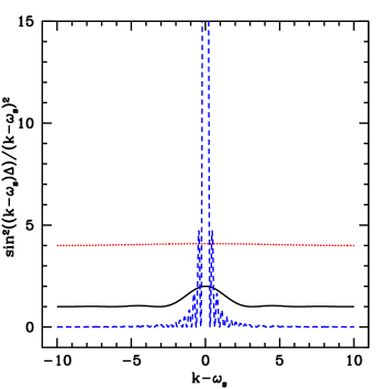
Figure 1: The quantity $\sin^{2}((k-\omega_{s})\Delta)/(k-\omega_{s})^{2}$, $\Delta=(t_{\rm fin}-t_{\rm in})/2$, is shown as a function of $k-\omega_{s}$ for the values of $\Delta=$ 1 (black, solid) 0.3 (red dotted) and 10 (blue, dashed). For clarity the red (dotted) and black (solid) curves are displaced.

Even though this flat space result cannot be taken over literally in a cosmological context, since we neglected the expansion of the universe, let us discuss in its lights, at least qualitatively, some examples of cosmological GW sources.

If turbulence is generated in the early universe during a first order phase transition, as discussed in the introduction, one has the formation of a cascade of eddies. The largest eddies have a period comparable to the time duration of the turbulence itself (of the phase transition). They are not spatially correlated, and are described by a wavenumber power spectrum which is peaked at a scale corresponding to their size. According to Eq. (16), these eddies generate GWs which inherit their wavenumber spectrum, since the last factor in this equation is flat enough, not to significantly influence the spectrum. Smaller eddies instead have higher frequencies, corresponding to periods smaller than the duration of the turbulence. According to Eq. (16), smaller eddies can imprint their frequency on the GW spectrum. However, they only contribute to the slope of the GW spectrum at high $k$: the peak of the GW spectrum is always dominated by the largest eddies. Therefore, the GW spectrum is peaked at a wavenumber corresponding to the size of the largest eddies.

Primordial magnetic fields are another cosmological source of GWs. They simply evolve by flux conservation and dissipation of energy at small scales, and have no characteristic oscillation frequency. Their lifetime is typically from their creation in the early universe until matter domination (after which only a negligible amount of GWs is produced caprini ; pedro ). Also in this case the wavenumber is imprinted in the induced GW spectrum. The suppression for $k(t_{\rm fin}-t_{\rm in})\gg 1$ is seen by the fact that GWs are generated mainly on super-horizon scales, $kt\lesssim 1$. Once a scale enters the Hubble horizon, further GW generation is negligible and the produced wave evolves simply by redshifting its frequency.

A similar case is represented by GWs produced by the neutrino anisotropic stresses, which generate a turbulent phase dolgov2 or simply evolve by neutrino free streaming  bashinsky . In the first case, the source is short lived and therefore its typical wavenumber is imprinted on the GW spectrum. In the second case there is no typical frequency and, like for magnetic fields, the relevant time is the time until a given wavenumber enters the horizon, $kt\simeq 1$. Again, the GW frequency corresponds to the source’s wave number.

A counter example is the stochastic GW background produced by binaries of primordial black holes which are copiously produced in some models with extra-dimensions bhb . In this case, one has a well defined typical frequency and the sources are long lived, so that $\omega_{s}(t_{\rm fin}-t_{\rm in})\gg 1$. The GWs inherit the frequency of the source.

IV Conclusions

To elucidate further our findings, let us consider again a spatially homogeneous source with well defined wave number $k$, which is alive only for a brief instant in time (a typical cosmological source). To determine the frequency of the generated GW, we observe it for some period of time (which is much longer than the inverse of the frequency). Since the source is active only for a very short period, as time goes on we observe GWs generated in different positions: what we see as happening in time, actually corresponds to a graviton-snapshot of the source in space, taken at the instant of time when it was on (see the bold solid lines in Fig. 2).

Conversely, for a source which occupies a very small spatial extension but lives for a long time (e.g. a binary star system), the situation is inverted. The GW signal arriving at the observer comes from virtually always the same position, but from different times. In this case the GW really monitors the time evolution of the source and therefore acquires its frequency (see the bold dashed lines in Fig. 2).

Figure 2: The past light cone (on which gravitons propagate) of a detector at $x=0$ observing for a given time interval sweeps a portion of space in the temporally confined source (solid, red line). Therefore, the wave number of the source is registered as the frequency of the emitted GW observed at $x$. On the other hand, the detector observes the time evolution of a spatially confined source (dashed, blue line), and therefore sees its frequency.

This duality between $k$ and $\omega$ is actually very natural, since they are related by Lorentz boosts. In general, both the spatial and time structure of a source lead to the generation of GWs.

In this brief report we have shown that the standard lore that GWs oscillate with the same frequency as their source is not always correct. Special care is needed in the cosmological context, where the universe has the same temperature everywhere and can undergo some drastic change simultaneously (but in a uncorrelated way) in a brief interval of time. This can lead to sources of GWs which are very extended in space, but short lived. Moreover, GWs from sources which only have a very slow time dependence and have no typical frequency, inherit usually the spectrum of the source in $k$-space.

In general, a source can have a complicated spectrum with structure in both $k$-space and frequency space. If the situation is not as clear cut as in the Gaussian wave packet, a detailed calculation is needed to obtain the correct GWs spectrum. On the top of that, as one sees explicitely in Eq. (5), only the values $({\mathbf{k}},\omega)$ with $|{\mathbf{k}}|=|\omega|$ of the Fourier transform of the source contribute to the GW amplitude.

References

- (1) N. Straumann, General Relativity With Applications to Astrophysics, Texts and Monographs in Physics, Springer (Berlin 2004), p. 248ff.
- (2) M. Kamionkowski, A. Kosowsky and M.S. Turner, Phys. Rev. D49, 2837 (1994).
- (3) A. Kosowsky, A. Mack and T. Kahniashvili, Phys. Rev. D66, 024030 (2002).
- (4) A.D. Dolgov, D. Grasso and A. Nicolis, Phys. Rev. D66, 103505 (2002).
- (5) A. Nicolis, Class. Quant. Grav. 21, L27 (2004).
- (6) A.D. Dolgov and D.Grasso, Phys. Rev. Lett. 88, 011301 (2001)
- (7) C. Caprini and R. Durrer, (2006) [astro-ph/0603476].
- (8) C. Grojean, G. Servant, (2006) [hep-ph/0607107].
- (9) C. Caprini and R. Durrer, Phys. Rev. D65, 023517 (2001).
- (10) R. Durrer, P. G. Ferreira and T. Kahniashvili, Phys. Rev. D61, 043001 (2000).
- (11) A. D. Dolgov and D. Grasso, Phys. Rev. Lett. 88, 011301 (2001).
- (12) S. Bashlinsky, (2005) [astro-ph/0505502].
- (13) K. T. Inoue and T. Tanaka, Phys. Rev. Lett. 91, 021101 (2003).