The Detailed Star Formation History in the Spheroid, Outer Disk, and Tidal Stream of the Andromeda Galaxy

Abstract

Using the Advanced Camera for Surveys on the Hubble Space Telescope, we have obtained deep optical images reaching stars well below the oldest main sequence turnoff in the spheroid, tidal stream, and outer disk of the Andromeda Galaxy. We have reconstructed the star formation history in these fields by comparing their color-magnitude diagrams to a grid of isochrones calibrated to Galactic globular clusters observed in the same bands. Each field exhibits an extended star formation history, with many stars younger than 10 Gyr but few younger than 4 Gyr. Considered together, the star counts, kinematics, and population characteristics of the spheroid argue against some explanations for its intermediate-age, metal-rich population, such as a significant contribution from stars residing in the disk or a chance intersection with the stream’s orbit. Instead, it is likely that this population is intrinsic to the inner spheroid, whose highly-disturbed structure is clearly distinct from the pressure-supported metal-poor halo that dominates farther from the galaxy’s center. The stream and spheroid populations are similar, but not identical, with the stream’s mean age being $\sim$1 Gyr younger; this similarity suggests that the inner spheroid is largely polluted by material stripped from either the stream’s progenitor or similar objects. The disk population is considerably younger and more metal-rich than the stream and spheroid populations, but not as young as the thin disk population of the solar neighborhood; instead, the outer disk of Andromeda is dominated by stars of age 4–8 Gyr, resembling the Milky Way’s thick disk. The disk data are inconsistent with a population dominated by ages older than 10 Gyr, and in fact do not require any stars older than 10 Gyr.

1. Introduction

One of the primary quests of observational astronomy is measuring the formation history of structures ranging in scale from individual galaxies to superclusters of galaxies. However, a serious impediment to this research is the fact that we live in a cosmological backwater. The Local Group hosts only two giant spiral galaxies, the Milky Way and Andromeda (M31, NGC 224), and no giant elliptical galaxies. The nearest galaxy groups to our own lie beyond 3 Mpc, with the closest (the Maffei Group) being heavily reddened (Karachentsev 2005).

Given our rural setting, it is not surprising that our own Galaxy drives the textbook picture of a giant spiral galaxy, with an ancient, metal-poor halo (e.g., Ryan & Norris 1991; VandenBerg 2000), an ancient, metal-rich bulge (e.g., Zoccali et al. 2003 ; McWilliam & Rich 1994), and a disk hosting a wide range of ages and metallicities (e.g., Fontaine et al. 2001; Ibukiyama & Arimoto 2002). However, stellar population work in the Milky Way is often limited by uncertainties in distance and reddening, and it is not even clear that the Milky Way is representative of giant spiral galaxies in general. Debate continues about the structure of the Milky Way system, how it formed, and how its various substructures (halo, bulge, disk, globular clusters, satellites, and tidal debris streams) formed with respect to one another. Physical processes possibly at work in forming the Milky Way include rapid dissipative collapse in the early universe (Eggen et al. 1962) and slower accretion of separate subclumps (Larson 1969; Searle & Zinn 1978). More recent hierarchical models suggest that spheroids form in a repetitive process during the mergers of galaxies and protogalaxies, while disks form by slow accretion of gas between merging events (e.g., White & Frenk 1991).

Although hierarchical models based on cold dark matter (CDM) show great success in reproducing the observable universe on scales larger than 1 Mpc, these models predict many more dwarf galaxies than are actually seen around the Milky Way (Moore et al. 1999). This discrepancy implies the existence of other mechanisms at work on small scales. For example, Bullock, Kravtsov, & Weinberg (2000) suggested that after the epoch of reionization, photoionization would suppress gas accretion in small subhalos, keeping most of them dark-matter dominated, and that a large fraction of those subhalos that did become dwarf galaxies would be tidally disrupted into the halos of their parent galaxies. However, Grebel & Gallagher (2004) argue that the presence of ancient stars in all dwarf galaxies, along with their wide variety of star formation histories, is evidence against a dominant evolutionary effect from reionization. Furthermore, Shetrone et al. (2003) demonstrated that chemical differences between nearby dSphs and the Galactic halo imply that the halo is not comprised of populations like those of present-day dSphs. Whether or not accretion of dwarf galaxies is the dominant source of stars in the halo, it is likely that such galaxies do contribute, and at large galactocentric distances their stars can remain in coherent orbital streams for 1 Gyr or more. The discovery of the Sgr dwarf (Ibata et al. 1994) rekindled interest in halo formation through accretion of dwarf galaxies, leading to ambitious programs to map the spatial distribution, kinematics, and chemical abundance in the halos of the Milky Way (e.g., Morrison et al. 2000; Majewski et al. 2000) and Andromeda (e.g., Ferguson et al. 2002; Guhathakurta et al. 2005). A spectacular example of this process has been found in Andromeda (Ibata et al. 2001), which hosts a giant tidal stream extending several degrees on the sky (McConnachie et al. 2003). Indeed, the star count map of Ferguson et al. (2002) shows complex substructure throughout Andromeda, while also showing evidence for an underlying smooth spheroid extending to large radii.

Besides the overabundant satellite problem, another issue with hierarchical CDM models is their prediction that gas loses much of its angular momentum during disk formation, resulting in theoretical disks that are much smaller than those observed (Navarro & Benz 1991). Some have turned to warm dark matter (WDM) cosmologies to alleviate this problem (e.g., Sommer-Larsen & Dolgov 2001), but there is an indication that angular momentum remains a problem in these models (see Bullock, Kravtsov, & Col$\acute{\rm i}$n 2002). Alternatively, the solution might lie in the inclusion of supernova feedback from the earliest generation of stars; recent models that show promise in this area predict that the bulk of the disk population was formed relatively late, at $z\lesssim 1$ (Thacker & Couchman 2001; Weil, Eke, & Efstathiou 1998), a prediction supported by panchromatic surveys of large numbers of galaxies (Hammer et al. 2005).

As the nearest giant spiral galaxy to our own, Andromeda offers an essential laboratory for studying the evolution of spiral galaxies. Given our vantage point, one might even argue that it is a better laboratory than our own Galaxy. At 770 kpc (Freedman & Madore 1990), the stars in Andromeda all appear to be at approximately the same distance, and at an inclination of $12^{\rm o}$ (de Vaucouleurs 1958), its various structures can be studied somewhat independently. We can resolve Andromeda’s old main sequence stars with the Hubble Space Telescope (HST), while the horizontal branch (HB) and upper red giant branch (RGB) are accessible to observatories on the ground. Recent years have seen an enormous increase in observing time directed at Andromeda, with deep pencil-beam surveys providing its star formation history (e.g., Brown et al. 2003; Brown et al. 2006; Stephens et al. 2003; Olsen et al. 2006) and shallow wide-field surveys providing maps of its morphology, metallicity, and kinematics (e.g., Ibata et al. 2001; Ibata et al. 2004; Ibata et al. 2005; McConnachie et al. 2003; Ferguson et al. 2002; Ferguson et al. 2005; Kalirai et al. 2006b; Guhathakurta et al. 2005).

At first glance, Andromeda and the Milky Way appear to be very similar; both are of similar Hubble type, luminosity, mass, and size (van den Bergh 1992; van den Bergh 2000; Klypin, Zhao, & Somerville 2002). However, we have long known that the Andromeda spheroid is very different from that of the Milky Way. The first evidence came from Mould & Kristian (1986), who found that the mean metallicity in the M31 halo, at 7 kpc on the minor axis, was surprisingly high ([m/H]$\approx-0.6$). Pritchet & van den Bergh (1994) subsequently found that the halo surface brightness profile, out to a distance of 20 kpc on the minor axis, follows a de Vaucouleurs exp$[-7.67(r/r_{e})^{1/4}]$ profile instead of the $r^{-2}$ power law expected for a canonical halo. These results were extended by Reitzel & Guhathakurta (2002), Durrell et al. (2001, 2004), and Bellazzini et al. (2003), who found that the high metallicity and de Vaucouleurs profile continued out to distances of 20–30 kpc on the minor axis. Recent surveys began probing M31 over much wider areas and much more deeply. Ferguson et al. (2002) mapped the density of bright RGB stars over 25 square degrees of the galaxy, finding significant substructure in the halo and outer disk. With photometry extending down to the oldest main sequence, Brown et al. (2003) reconstructed the star formation history in the halo at 11 kpc on the minor axis, and found a wide age distribution, with $\sim$30% of the stars at ages of 6–8 Gyr. All of these studies suggested that the M31 halo is dramatically different than the Milky Way halo, begging the question “which is representative of large spiral galaxies?” One possible answer comes from Mouhcine et al. (2005), who found that the metallicities of spiral halos correlate well with their parent galaxy luminosities; the Milky Way halo falls well off this metallicity-luminosity relation (being unusually metal-poor for the parent galaxy mass), while the M31 halo appears representative for large spiral galaxies. It is unclear if this trend is due to a general tendency for more massive galaxies to host a more dominant bulge, ingest more satellites, and/or ingest larger satellites.

Recently, two independent groups (Guhathakurta et al. 2005; Irwin et al. 2005) studying the outskirts of M31 found an extended stellar halo that more closely resembles the halo of our own Milky Way. This extended halo begins to dominate beyond 30 kpc, where the minor-axis surface-brightness profile transitions from a de Vaucouleurs law to an $r^{-2.3}$ law. From the colors in their photometric sample, Irwin et al. (2005) concluded that the metallicity in the extended halo was as high as it is in the region interior to 30 kpc, but Guhathakurta et al. (2005), using a spectroscopically-confirmed sample extending 3 times farther out on the minor axis, found that this extended halo is metal poor. However, the existence of a metallicity gradient was later confirmed by Kalirai et al. (2006b). These discoveries can lead to a confusion of terminology. It seems straightforward to refer to the inner few kpc as the bulge, and to the stars beyond 30 kpc as the halo, but what about the stars at 5–30 kpc on the minor axis? Before the discovery of the extended metal-poor halo, this population of metal-rich stars was generally referred to as the halo, but it is quite possible that this stellar population is more closely related to the bulge. Furthermore, there has been considerable debate about the contribution of disk stars at these radii. Kinematic studies indeed show that M31 has an extended thick disk (Ibata et al. 2005). The minor-axis population at 11 kpc from the center has kinematics that are inconsistent with a rotationally supported disk (Kalirai et al. 2006b; Rich et al. in prep.), but the velocity dispersion is smaller than might be expected for a purely pressure-supported stellar system. Because the term “spheroid” normally refers to a structure that includes the bulge and halo, we use the term here when referring to the extraplanar stars at 5-30 kpc, merely to distinguish from those regions that can be clearly labeled bulge (within $\sim$5 kpc of the nucleus), disk (within $\sim$30 kpc on the major axis), and halo (beyond $\sim$30 kpc on the minor axis). However, our use of this term is not intended to imply a smooth, relaxed, pressure-supported structure.

To further understand the formation of Andromeda, we need to know the star formation histories of its various structures. To that end, we have now obtained deep HST images in three fields, located in the inner spheroid, outer disk, and the giant tidal stream. All of these images reach well below the oldest main sequence turnoff (MSTO) in the galaxy, allowing a reconstruction of the entire star formation history in each field. Keck spectroscopy in each of these fields provides additional kinematic information (Kalirai et al. 2006b; Reitzel et al. 2006, in prep; Rich et al. 2006, in prep). In previous papers (Brown et al. 2003; Brown et al. 2006) we presented the preliminary analysis of the spheroid and stream fields. In this paper, we present the detailed star formation histories in the spheroid, stream, and outer disk of Andromeda. In §2, we describe our observing strategy and the data. We describe the data reduction in §3, followed by the production of the photometric catalogs in §4. In §5, we describe our analysis, which ranges from qualitative inspection of the color-magnitude diagrams (CMDs) to quantitative fitting of the star formation histories, including a full exploration of the possible systematic effects of our assumptions. In §6, we discuss the implications of our analysis. The results of our study are summarized in §7.

2. Observations

Using the Advanced Camera for Surveys (ACS; Ford et al. 1998) on HST, we obtained deep optical images of three fields in M31: the spheroid, outer disk, and tidal stream (Figure 1; Table LABEL:fieldtab). We used the F606W (broad $V$) and F814W ($I$) filters on the Wide Field Camera (WFC). The spheroid data, obtained in the first HST observing cycle with ACS, reach their goal of $\sim$1.5 mag below the oldest MSTO, while the stream and disk data, obtained two years later, reach their goal of $\sim$1.0 mag below the oldest MSTO.

Table 1Field Characteristics

	R.A.	Dec.	log $N_{HI}$	F606W	F814W
Field	(J2000)	(J2000)	(1019 cm-2)	(ksec)	(ksec)	Date
spheroid	00:46:07.1	40:42:39	19.3	139	161	2 Dec 2002 – 1 Jan 2003
stream	00:44:18.2	39:47:32	$<17.6$	53	78	30 Aug 2004 – 4 Oct 2004
disk	00:49:08.6	42:45:02	20.6	53	78	11 Dec 2004 – 18 Jan 2005
aBraun et al. in prep; D. Thilker, private communication.
bThilker et al. (2004).

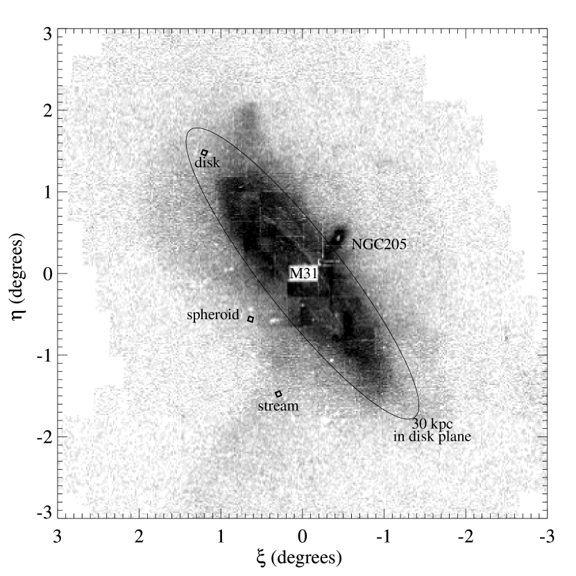
Figure 1.— A map of stellar density in the Andromeda vicinity, from counts of RGB stars (Ferguson et al. 2002). Appropriately scaled and rotated boxes denote our three fields (labeled). An ellipse marks the area within 30 kpc of the galactic center in the inclined disk plane (labeled).

The original spheroid program was proposed before the installation of ACS on HST, and at that time, no images of M31 had reached significantly below the level of the HB (3 mag brighter than an old MSTO). Given the uncertainties in this situation, our goal was an ambitious depth that would unambiguously characterize the star formation history in the spheroid. With the proven capabilities of ACS and the success of this program, we subsequently proposed a less conservative approach as far as depth was concerned, giving up 0.5 mag of depth for the ability to explore two fields without increasing the size of the observing program.

Surface brightness was the primary driver in field selection. There are two competing factors in obtaining a CMD appropriate for reconstructing the star formation history. One wants to maximize the number of stars in the CMD, to minimize contamination from foreground stars and background galaxies, to minimize statistical uncertainties in the characterization of the population, and to allow the detection of subtle CMD features (e.g., small bursts due to interaction of Andromeda with its satellites). One also wants to minimize the crowding, in order to maximize the accuracy of the photometry for a given exposure time. To explore these competing factors, we created realistic simulations of ACS images under various population assumptions, and found that the optimal crowding is approximately one star of interest for every 50–100 resolution elements; these results agree well with those of Renzini (1998). The native ACS/WFC pixel size is 0^′′.05, which is approximately twice the width for critically sampling the point spread function (PSF), so the number of resolution elements is roughly the number of pixels. This translates into $\sim$250,000 stars in an ACS image, corresponding to a surface brightness $\mu_{V}\approx$26.3 mag per square arcsec, which defines a roughly elliptical isophote around M31 that provides the optimal crowding.

Fortuitously, the intersection of this isophote with the southern minor axis falls near a globular cluster (SKHB-312) previously imaged with the Wide Field Planetary Camera 2 (WFPC2) on HST (Holland et al. 1997), so the exact position of our spheroid image was chosen to place this cluster at the edge of our field. Holland et al. (1996) determined the metallicity distribution in this field, and showed that it was very similar to that observed in other fields throughout the inner spheroid. Although Holland et al. (1997) reported a 10^′′ tidal radius for this cluster, we placed it at the edge of our field in case deeper images revealed a larger extent to the cluster that would contaminate a significant fraction of the image and negatively impact the primary goal of studying the field population. Our photometry of SKHB-312 reached well below its MSTO, revealing a cluster age of 10 Gyr (Brown et al. 2004b). Brown et al. (2004b) found no evidence for extended tidal tails in the cluster, and so for the current study, we mask the area within 15^′′ of the cluster center. In the subsequent observations of the tidal stream and outer disk, there was only a candidate globular cluster (Bol D242; Galleti et al. 2004) near our optimal position in the stream, and no known globular clusters near our optimal position in the disk. The exact location of the stream field was chosen to include this candidate cluster (which subsequently turned out to be a superposition of foreground stars), whereas the exact location of the disk field was chosen to minimize the contribution from the spheroid, based upon the disk/spheroid decomposition of Walterbos & Kennicutt (1988). The surface brightness in the stream field is $\approx$0.5 mag fainter than that in our original spheroid program, while that in the disk field is $\approx$0.1 mag brighter than that in our original spheroid program. The hydrogen column density in the disk field is also much larger than that in the spheroid and stream fields (see Table LABEL:fieldtab for $N_{HI}$ measured at each of our field positions).

Each exposure in a given bandpass was dithered so that no two exposures placed a star on the same pixel. Dithering smooths out sensitivity variations across the detector, fills in the gap between the two halves of the ACS/WFC detector, allows optimal sampling of the PSF, and enables the removal of hot pixels. Our dither pattern employed three tiers of dithers to optimize the data quality. The first two tiers determined the nominal field position for one of our visits in a given band (usually spanning two orbits), while the final tier provided a 4-point dither pattern to optimally sample the PSF within a visit. The offsets in the first dither tier moved from -5 to +10 pixels in X, with steps of 5 pixels, and from +60 to -120 pixels in Y, with steps of 60 pixels, to place the detector gap at four adjacent positions on the sky. These first-tier offsets produce four horizontal strips in our data where the field is underexposed by 25%; stars in these strips are ultimately discarded from our catalog, but sampling the sky in the detector gap yields more accurate PSF-fitting for the field because we have contiguous photometry for all of the objects in the field. The offsets in the second dither tier moved -4.5, 0, or +4.5 pixels independently in X and Y, to smooth out small-scale variations in detector response, plus a random fractional pixel in X and Y, to avoid aliasing effects between the various dithers, the pixel plate scale, and the geometric distortion. The offsets in the third tier were (0,0), (+1.5,0), (+1.5,+1.5), and (0,+1.5) pixels in X and Y, to sample the PSF at twice the frequency provided by a single exposure.

Each of these programs obtained brief exposures of Galactic star clusters with the same filters on the ACS/WFC (Table 2; Brown et al. 2005). The resulting CMDs provide empirical isochrones that can be compared directly to the Andromeda CMDs and used to calibrate the transformation of theoretical isochrones to the ACS bandpasses. These cluster observations, the empirical isochrones, and the transformation of the theoretical Victoria-Regina Isochrones (Vandenberg, Bergbusch, & Dowler 2006) to the ACS bandpasses are fully detailed by Brown et al. (2005). We will use these empirical isochrones and theoretical isochrones here, shifted to the Andromeda reference frame by assuming a distance of 770 kpc (Freedman & Madore 1990) and a reddening of $E(B-V)=0.08$ mag (Schlegel, Finkbeiner, & Davis 1998). Over the region defined for fits to the star formation history, the theoretical isochrones agree with the observed cluster CMDs at the 0.02 mag level.

Table 2Parameters of Galactic clusters observed with ACS

	$(m-M)_{V}$	$E(B-V)$		age
Name	(mag)	(mag)	[Fe/H]	(Gyr)
NGC 6341 (M92)	14.60	0.023	$-2.14$	14.5
NGC 6752	13.17	0.055	$-1.54$	14.5
NGC 104 (47 Tuc)	13.27	0.024	$-0.70$	12.5
NGC 5927	15.85	0.42	$-0.37$	12.5
NGC 6528	16.31	0.55	$+0.00$	12.5
NGC 6791	13.50	0.14	$+0.30$	9.0
aBrown et al. 2005 and references therein.

A sample of bright RGB stars in our three fields has been observed spectroscopically with Keck, providing crucial kinematic context for each field. The velocity data in all three fields are presented by Kalirai et al. (2006b), but the focus of that paper is the kinematic structure of the tidal stream. Rich et al. (2006, in prep.) will focus on the kinematic structure of the spheroid, while Reitzel et al. (2006, in prep.) will focus on the kinematic structure in the outer disk. The velocity information in each of our fields is presented in Figure 2. The velocities in the spheroid field show a broad distribution, with no dominant contribution from a disk or a single stream. The velocities in the stream field show it to be dominated ($\approx 3/4$) by stars moving in two narrow stream components, with the remainder in the spheroid. The velocities in the disk field show it to be dominated ($\approx 2/3$) by stars moving in a disk component, with the remainder in the spheroid.

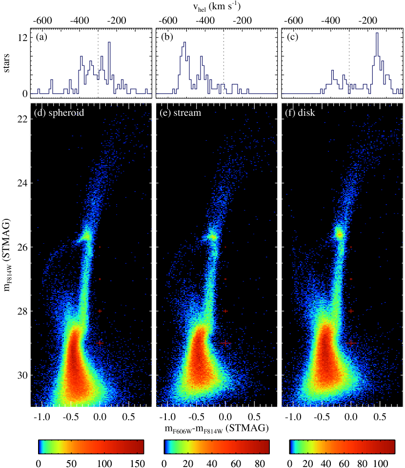
Figure 2.— The velocities (upper panels) and CMDs (lower panels; Hess diagrams at a logarithmic stretch) for our three fields, with representative error bars (red crosses to the right of the stellar locus). Scales under each CMD indicate the number of stars per bin. The velocity histogram for our spheroid field (a) shows a broad distribution ($\sigma\approx 80$ km s^-1) at the Andromeda systemic velocity (dashed line), with no significant contribution from a disk or single stream (Rich et al. in prep.). The stream field (b) is dominated by two kinematically-cold ($\sigma\approx 15$ km s^-1) stream components, falling toward the observer from behind the galaxy, with the remainder in a broader spheroid component at the systemic velocity (Kalirai et al. 2006b). The disk field (c) is dominated by a narrow disk component, redshifted due to the rotation of the disk, with the remainder in a broader spheroid component at the systemic velocity (Reitzel et al. in prep). The populations in the spheroid (d) and stream (e) look remarkably similar (Brown et al. 2006), although the spheroid data are 0.5 mag deeper. The disk, in contrast, shows a younger population (note the red clump HB morphology and the blue plume above the dominant MSTO) at higher mean metallicity (note the redder RGB). Figures 6 and 7 highlight the distinctions among the three populations.

3. Data Reduction

If calibrated data are retrieved from the HST archive as soon as they are available, they will generally not have the best dark and bias subtractions, because those calibration products are created weeks later from a contemporaneous set of data that was obtained in the days surrounding a given observation. Thus, months after these observations, we re-retrieved the images, yielding data with the latest ACS pipeline calibration, including an appropriate dark subtraction, flat-field, and bias correction; these are the “FLT” files in the ACS pipeline. We then subtracted an iteratively sigma-clipped median sky level from each quadrant of each image to avoid an unnecessary increase in image noise during the later coaddition of the images; this also corrects for small quadrant-dependent bias residuals. We used the PyRAF DRIZZLE package (Fruchter & Hook 2002) to register the individual images, correct for geometric distortion and plate scale variations, reject cosmic rays, and coadd all of the frames in a given bandpass. The geometric distortion correction employed the coefficients provided by the ACS calibration pipeline for each image, which include both the general geometric distortion and also the time-varying plate scale changes due to velocity aberration. As part of the drizzle process, the images were resampled to a plate scale of 0^′′.03 pixel^-1. Residual shifts, rotations, and plate scale variations were corrected as part of our registration process, and thus our reduction is immune to the software errors that have sometimes caused registration and photometry problems in the MULTIDRIZZLE software (although note that we do not use MULTIDRIZZLE in our reduction).

To register the images, we drizzled the images to individual output frames that were corrected for geometric distortion and velocity aberration, with relative shifts determined by the pointing information in the image headers (closely matching our commanded dither pattern). The positions of $\sim$10,000 relatively bright stars, well-detected in the individual images, were then measured in each image through the entire image stack, using an iterative fit of a Gaussian profile to each star. These stellar positions were used to refine the offsets (deviations from the guide star offsets), rotations (deviations from the fixed orientation requested), and plate scale changes (telescope breathing and residual velocity aberration). Using the refined knowledge of the relative astrometry, we re-drizzled the images to individual output frames. These refinements to the offsets, rotations, and scales are iterated until the positions of the bright stars in the individual images are aligned to better than 0.01 pixels.

Next we created masks of cosmic rays and problematic pixels. Although saturated pixels are masked in the data quality array (along with some of the hot and dead pixels), saturation is only an issue for the handful of bright foreground stars and not stars in M31; in our half-orbit exposures, a star would have to be brighter than 20.6 mag in either bandpass and well-centered in a pixel for saturation to occur. To create our masks, we first calculated a clipped median of all the images in a given band, resulting in our first pass at the deep image in that band. The first-pass images were then reverse-drizzled (or “blotted” in the drizzle nomenclature) back to the original frame of the individual images. The comparison of these blotted images with each FLT image enabled the creation of masks for the cosmic rays, self-annealed pixels (oversubtracted by the dark calibration), and short-term transient warm and hot pixels not corrected by the contemporaneous dark calibration. To create a complete mask for each frame, these custom masks were combined with the pipeline-provided data quality masks in which we include all pixels flagged for any reason. The masked images were then coadded, with weighting by exposure time, to create a second-pass deep image in each band. Because this iteration was significantly improved over the first pass (median image), these second-pass deep images were then blotted back to the original frames of the individual images, to enable refinement of the image masks. The frames were coadded a third time to create the final image in each bandpass. We then added a flat sky component to each final image, representing the exposure-weighted mean of the sky background subtracted from the individual frames, to ensure that the counting statistics were appropriate in the subsequent photometric reduction. In Figure 3, we show a false-color $30^{\prime\prime}\times 30^{\prime\prime}$ subsection of our spheroid field, combining the images in F606W and F814W filters.

Figure 3.— A $30^{\prime\prime}\times 30^{\prime\prime}$ subsection of our spheroid field, with a logarithmic stretch. The blue channel comes from the F606W exposure, the red channel comes from the F814W exposure, and the green channel comes from the sum of those two bands. A yellow box marks a star near the MSTO, at $m_{F814}=29$ mag, $m_{F606W}-m_{F814W}=-0.45$ mag; it is clear that stars are detected well below this point. This subsection was chosen to give examples of the types of objects in our field – Galactic foreground stars (with diffraction spikes), background galaxies, and Andromeda stars – but it is not a typical patch. Most of the image is dominated by Andromeda stars.

Although this process was repeated on the full set of data for each field, we also applied the process to a subset of the spheroid data chosen to match the shorter exposure times in the stream and disk. In this paper, the fits to the star formation history in the spheroid utilize the full dataset, but the shallower version of the spheroid data is useful for making a fair comparison of the CMDs of the three fields. Spheroid CMDs utilizing this subset of the data are labeled “matched.”

4. Photometry

We used the DAOPHOT-II (Stetson 1987) PSF-fitting package to obtain photometry of each field. Empirical PSFs were created from the images using the most isolated and well-exposed stars, with a radius of 23 pixels (0^′′.69). We first performed an initial pass of object detection and aperture photometry. The resulting object catalog was then clipped to retain only those well-detected stars that fell within the dominant stellar locus in the CMD (rejecting outliers that are obvious blends and background galaxies), while also avoiding those stars near the tip of the RGB and in the instability strip (which can be variable and thus have PSFs adversely affected by the cosmic-ray cleaning). We then screened for stars with relatively bright neighbors; to be a valid PSF star, all neighbors within 15 pixels must be at least 3 mag fainter than the PSF star, and all neighbors within 22 pixels must be at least 2 mag fainter than the PSF star. Finally, we created a SExtractor (Bertin & Arnouts 1996) map of the thousands of background galaxies in our image, and removed from our list of PSF candidates any star within 23 pixels of an extended object. We also removed stars within 23 pixels of an image border or a bad pixel (e.g., due to charge bleeding from saturated stars). This resulted in $\sim$2000 PSF candidates per field in the disk and spheroid and $\sim$1600 PSF candidates in the stream field. These PSF stars were then passed through an iterative process to create the empirical PSF for each bandpass in each field. In the first pass, we used the PSF of Brown et al. (2003) as an initial guess at the current PSF. We fitted this PSF to the catalog of stars, subtracted those stars, and then performed a new round of object detection on the residual image to find the fainter stars uncovered. We added these stars to the catalog, and repeated the PSF-fitting photometry for the entire catalog. Stars neighboring each PSF star were then subtracted, and a new PSF was then created. During this process, we eliminated PSF stars whose fits were high $\chi^{2}$ outliers (as reported by DAOPHOT-II). Also PSF stars were cut from the list if PSF subtraction uncovered close stellar blends with the PSF star or revealed underlying deviant pixel artifacts. Using such a large number of PSF stars, we are able to compare the morphology of the PSF-subtracted residuals to those of nearby PSF stars and reject any with morphology deviating from the pattern in that particular region of the image. This process was iterated, each time increasing the allowed degree of spatial variability in the fit, starting from a spatially-constant PSF and ending at a third-order polynomial variation with field position. This degree of variability is an advantage of the stand-alone DAOPHOT-II code, as the IRAF version only allows a second-order trace of the strong spatial variation in the ACS/WFC PSF. Once we stopped increasing the degree of spatial variability in the PSF, we iterated two more times, purging problematic PSF stars after each new round of PSF production, until an accurate spatially-varying PSF was created for each bandpass in each field. In the end, $\sim$1600 stars were used to create the PSF in the disk and spheroid fields, while $\sim$1400 stars were used in the stream field.

With the empirical PSFs in hand, we performed PSF-fitting photometry on the images to create the catalog of stars in each field. First, we used the “find” routine in the DAOPHOT-II package and a 5$\sigma$ detection threshold on the sum of the F606W and F814W images, to create the initial pass at object detection. After making an initial estimate of magnitudes for the catalog with a round of aperture photometry in each band, the catalog was cleaned of PSF substructure misidentified as stars in the vicinity of well-exposed stars. The aperture photometry was then used as the starting point for PSF-fitting photometry. After these stars were fitted and subtracted from each image, we summed the residual images in F606W and F814W to create a new detection image, which was again fed to the find routine with a 5$\sigma$ threshold. The detections in this second pass were often noise residuals from the subtraction of the stars in the first pass, or other image artifacts revealed by the subtraction. Our first screen of these artifacts was made using the sharpness measurement produced by the find algorithm. We cut 4$\sigma$ outliers in the sharpness distribution. We then screened artifacts from bright star residuals (consistent with Poisson noise) by removing detections within a given magnitude-dependent radius of stars in the first-pass catalog; the radius is magnitude-dependent because for fainter stars, the residuals approach sky noise at a smaller radial distance from the center of the PSF. We obtained aperture and then PSF-fitting photometry of the second-pass stars, without re-centering, using the original F606W and F814W images (i.e., the deep drizzled images as they stood before any PSF subtractions). The first-pass and second-pass star lists were then combined, and another run of PSF-fitting photometry (now allowing recentering) was performed on the original F606W and F814W images. DAOPHOT-II reports a goodness-of-fit ($\chi^{2}$) statistic for the PSF fits to each star; we analyzed the distribution of this $\chi^{2}$ statistic as a function of stellar magnitude, and marked those objects in the deep images that had high $\chi^{2}$ values. Inspection of the marked images showed that these outliers were primarily due to close blends, PSF artifacts (e.g., diffraction spikes), and/or objects superimposed on background galaxies (which include both true Andromeda stars superimposed on background galaxies and substructure within background galaxies incorrectly identified as stars). We clipped from the catalog these outliers in the $\chi^{2}$ distribution. This clipping is responsible for much of the improvement between the CMDs shown here and that shown in the preliminary publication of the spheroid CMD (Brown et al. 2003). Finally, we discarded those stars falling in parts of the image without the full exposure (due to dithering the image edges and the detector gap). Note that our artificial star tests (discussed below) included all of the same processes and evaluations used in the process that created the photometric catalog, so that any rejection of real stars is reproduced in the simulated CMDs.

The PSF-fitting photometry was put on an absolute magnitude scale by normalizing to aperture photometry on the brightest stars. That aperture photometry was itself put on an absolute magnitude scale using aperture corrections determined from TinyTim (Krist 1995) models of the ACS PSF. The aperture corrections were verified with observations of the standard star EGGR 102 (a $V=12.8$ mag DA white dwarf) in the same filters; the agreement between the standard star photometry and the TinyTim model is at the 1% level. In Figure 2, we show the CMD for each field at its full depth, along with the associated velocity distribution of RGB stars in each field (Kalirai et al. 2006b; Rich et al. in prep; Reitzel et al. in prep.). Due to the large numbers of stars in each field, a traditional CMD (with a point for every star) is saturated and difficult to interpret; instead, we have binned the data into Hess diagrams, with shading indicating the number of stars per bin. The same logarithmic stretch (characterized by the scales under each CMD) spans the full range of stellar density in each CMD, but that range varies from field to field given the variation in surface brightness and observing depth. The stretch was chosen to reveal both the subtle and gross properties of each population. We also plot representative errors bars in each CMD, measured by taking the standard deviation between the input and output values for the given color and magnitude in our artificial star tests (discussed below); note that crowding is the dominant source of scatter in each bandpass, which causes photometric errors to be larger in either $m_{F606W}$ or $m_{F814W}$ than in $m_{F606W}-m_{F814W}$.

Our photometry is in the STMAG system: $m=-2.5\times$ log${}_{10}f_{\lambda}-21.1$ mag, where $f_{\lambda}=$ e${}^{-}\times{\rm PHOTFLAM/EXPTIME}$, EXPTIME is the exposure time, and PHOTFLAM is $7.906\times 10^{-20}$ erg s^-1 cm^-2 Å^-1 / (e^- s^-1) for the F606W filter and $7.072\times 10^{-20}$ erg qs^-1 cm^-2 Å^-1 / (e^- s^-1) for the F814W filter. The STMAG system is a convenient system because it is referenced to an unambiguous flat $f_{\lambda}$ spectrum; an object with $f_{\lambda}=3.63\times 10^{-9}$ erg s^-1 cm^-2 Å^-1 has a magnitude of 0 in every filter. Another convenient and unambiguous system that is widely used is the ABMAG system: $m=-2.5\times$ log${}_{10}f_{\nu}-48.6$ mag; it is referenced to a flat $f_{\nu}$ spectrum, such that an object with $f_{\nu}=3.63\times 10^{-20}$ erg s^-1 cm^-2 Hz^-1 has a magnitude of 0 in every filter. It is thus trivial and unambiguous to convert any of the data presented herein from STMAG to ABMAG: for F606W, ABMAG = STMAG $-$ 0.169 mag, and for F814W, ABMAG = STMAG $-$ 0.840 mag. Although our photometry could be transformed to ground magnitude systems (e.g., Johnson $V$ and Cousins $I$) for comparison to theoretical isochrones as well as other data in the literature, such transformations always introduce significant systematic errors (see Sirianni et al. 2005). Instead of converting HST data to ground bandpasses, it is preferable to produce models in one of the HST instrument magnitude systems, in either STMAG or ABMAG.

Brown et al. (2006) found excellent agreement between the HB and RGB distributions in the stream and spheroid populations if the stream is assumed to be 0.03 mag (11 kpc) more distant than the spheroid. The sense of the offset in luminosity is in agreement with the velocities of the stars in the stream, which imply that the stream is falling into Andromeda from behind it (Figure 2b; see also McConnachie et al. 2003). Brown et al. (2006) also found a 0.014 mag offset in color between the stream and spheroid data, which is well within the uncertainties in calibration and reddening. Thus, we shifted the stream CMD 0.03 mag brighter and 0.014 mag to the red, to put it in the same frame of reference as the spheroid data. These shifts are very small, and make very little difference to the CMDs displayed herein or to the various fits to the stream data, but we apply these shifts because they are appropriate to the best of our knowledge. The distinctions between the spheroid and disk CMDs are far larger than the calibration and reddening uncertainties, and in fact no single shift in color and luminosity can align the features of the disk and spheroid CMDs. Thus, to the best of our knowledge, the distinctions between the disk and spheroid data are physical, and so the disk data are analyzed without modification.

It is worth noting the implications of our shifts to the stream data if these shifts are entirely due to a difference in extinction. The Schlegel et al. (1998) extinction map gives $E(B-V)=0.08$ mag at our spheroid and disk positions and $E(B-V)=0.05$ mag at our stream position, but this variation is within the uncertainties for their map, which are generally $\sim 0.02$ mag in random fields and a bit higher near Local Group galaxies. At 3,500 $\leq T_{\rm eff}\leq$ 35,000 K, synthetic spectra folded through the ACS and ground bandpasses imply $E(m_{F606W}-m_{F814W})\approx E(B-V)$. So, if we took the map at face value, we would shift the stream data 0.03 mag to the red and 0.05 mag fainter, to put the stream data in the same extinction reference frame as the spheroid data. However, a 0.03 mag shift to the red is larger than the 0.014 mag required to align the stream and spheroid color distributions at the HB and RGB. Given the uncertainties in the extinction map, we could instead shift the stream data 0.014 mag to the red and 0.02 mag fainter. This would align the color distributions of the stream and spheroid at the HB and RGB, but the stream HB would be $0.03+0.02=0.05$ mag fainter than the spheroid HB, implying that the stream distance modulus in our field is 0.05 mag larger than the spheroid distance modulus. In any case, given that the calibration uncertainties for the $m_{F606}-m_{F814W}$ color are also at the same level as the color shift, it is not appropriate to read too deeply into these small shifts in color and magnitude between the fields.

Damage to the CCDs due to radiation in space leads to charge transfer inefficiency (CTI), a problem that is particularly noticeable in large-format CCDs. CTI causes stars to appear fainter than they actually are. The ACS WFC detector consists of two chips, with $4096\times 2048$ imaging pixels each, separated by a small gap. Each CCD is read out through two serial amplifiers, with 24 physical pixels of leading serial overscan for each and 20 rows of trailing virtual overscan in the parallel clocking direction, yielding a final downlinked image format of $4144\times 2068$ for each CCD. Stars that fall closer to the gap undergo more parallel transfers when the detector is read, and thus suffer from more charge loss due to CTI (for these CCDs, at the ACS operating temperature and clocking rates, the CTI effects after radiation exposure are much more significant in the parallel clocking direction than in the serial). The CTI correction is approximately linear with the position of a star relative to the gap, and approximately linear with the age of the detector. The correction is larger for faint stars and smaller when there is a significant background. Our spheroid field was observed shortly after the ACS launch, while the stream and disk fields were observed two years later. The standard CTI correction (Riess & Mack 2005) was derived for brighter stars with lower backgrounds than the situation in our images. Thus, it is somewhat uncertain whether or not one should extrapolate these CTI corrections into the regime of our data, which includes the deepest stellar photometry obtained with HST to date. Fortunately, CTI does not appear to be a significant problem in our images. We checked the effects of CTI by constructing CMDs of stars extracted from a range of horizontal bands across the image. The CMD includes two horizontal features separated by approximately 3 mag in luminosity: the HB and the subgiant branch (SGB). The luminosity of each of these features can be determined by taking a vertical cut through the CMD in the vicinity of each feature (using a region restricted in color to avoid other evolutionary phases). If CTI were a significant problem in our data, one would expect the luminosity offset between the HB and SGB to vary by a few hundredths of a magnitude as a function of vertical position in the image, given the intensity of the sources and the observed sky background. In reality, we find that this offset varies by $\lesssim$0.001 mag across the image. Thus, there are probably additional factors contributing to the CTI mitigation, besides the sky background of $\sim$100 counts per pixel. Because the images are crowded with stars and background galaxies, most stars are clocked across pixels where the charge traps have already been filled by other sources. Given the lack of evidence for CTI, we do not attempt a CTI correction. Note that any CTI correction applied to these data would tend to make the stellar populations look slightly younger, because the fainter main sequence and subgiant stars would have a larger correction than the brighter HB stars.

We next performed extensive artificial star tests to characterize the completeness and photometric scatter as a function of color and magnitude in each field. These tests required months of computations on a dedicated cluster of 10 processors. In all, 5 million artificial stars were added to each field and blindly recovered, with these stars spanning the full range of color and magnitude populated by the stellar locus. These stars were added in 1000 passes with 5000 stars per pass, to avoid significantly increasing the crowding in the images. The artificial stars were blindly recovered with a process identical to that used for the photometric catalog. The completeness exceeds 80% at $m_{F814W}\leq 30.5$ mag in the spheroid data, and exceeds 80% at $m_{F814W}\leq 30.0$ mag in the disk and stream data, but it drops off rapidly below these magnitudes. These limits drive the faint limit of the region we fit for the star formation history. Note that the images detect stars significantly fainter than those presented in the CMDs presented here; compared to the reduction of Brown et al. (2003), the catalog depth and completeness have been somewhat reduced by the higher detection threshold and rigorous cleaning process we have employed here.

5. Analysis

5.1. Inspection of the Color-Magnitude Diagrams

Before turning to the quantitative fitting of the CMDs, much can be learned from simple visual inspection. The CMD for the population in each field is shown in Figure 2. At first glance, all three CMDs look remarkably similar, even though the populations have distinct kinematics. All of them show a broad RGB, indicative of a wide metallicity range. In each field, the majority of the stars between the MSTO and the base of the RGB are clustered in a tight locus. Given the spread in metallicity, this tight SGB locus indicates a wide range in age, with younger stars generally more metal-rich than older stars. A minority population of stars appears in a blue plume above the MSTO, representing a young population with a wide range of metallicities. We return to the SGB and blue plume below. Each of the fields has a well-defined HB, although the HB in the disk field is largely restricted to a red clump, while in the stream and spheroid $\sim$10% of the HB stars fall on the blue end of the HB. None of the fields have an extended hot HB, as seen in massive Galactic globular clusters spanning a wide range in metallicity (e.g., M19, at [Fe/H] = $-1.68$, and NGC6441, at [Fe/H] = $-0.53$; Piotto et al. 1999; Rich et al. 1997). Instead, the blue HB, when present, very closely resembles that of typical metal-poor clusters, such as M92, at [Fe/H] = $-2.1$ (see Brown et al. 2003). The RGB luminosity function bump is prominent in each CMD, at a luminosity $\sim$0.5 mag fainter than the red end of the HB; this bump is a metallicity indicator, becoming fainter (relative to the HB) at higher metallicities, and in all three fields its spread in luminosity is another indication of a spread in metallicity. None of the CMDs shows multiple discrete turnoffs, as might be expected from pulses of star formation.

In Figure 4, we compare the CMDs to our globular cluster fiducials (Table 2; Brown et al. 2005). Due to their wide range of metallicities, the clusters span most of the RGB width in the M31 CMDs. However, because the clusters are old, there is an obvious trend for the MSTO and SGB in the more metal-rich clusters to be too faint relative to those features in the M31 CMDs. In the bottom panels of Figure 4, we show a comparison of the M31 CMDs to calibrated isochrones at three different ages (3, 8, and 13 Gyr) and three different metallicities ([Fe/H] = 0, $-1$, and $-2$). It is clear that the old ($>10$ Gyr) populations in these fields must be predominantly metal-poor ([Fe/H]$\leq-1$), and that the metal-rich populations ([Fe/H]$>-1$) must be of intermediate age ($\sim 6$–8 Gyr). An old metal-rich population would have a MSTO much redder and fainter than observed, while an intermediate-age metal-poor population would have a MSTO much bluer and brighter than observed. That said, there is a minority population of young stars spanning a wide range in metallicity, with the brightest and bluest stars in the plume matched by the 3 Gyr isochrone at [Fe/H] = $-2$.

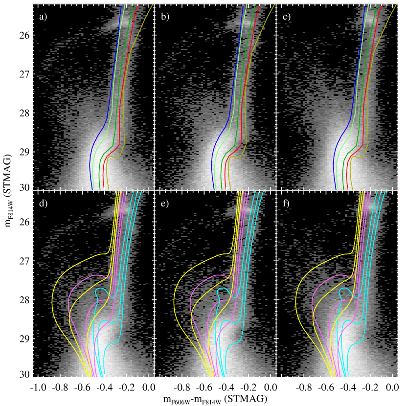
Figure 4.— Top panels: The CMDs of the spheroid ($a$), stream ($b$) and disk ($c$), compared to the ridge lines of the Galactic globular clusters in Table 2 (colored curves). The Andromeda data are shown as Hess diagrams with the same binning used in Figure 2, but over a narrower range of color and luminosity. The ridge lines shift redward with increasing cluster metallicity. Bottom panels: The CMDs of the spheroid ($d$), stream ($e$) and disk ($f$), compared to isochrones at [Fe/H] = $-2$ (yellow curves), $-1$ (pink curves), and 0 (light blue curves), and ages of 3, 8, and 13 Gyr (running from left to right for each color). It is clear that the old ($>10$ Gyr) populations in these fields must be predominantly metal-poor ([Fe/H]$\leq-1$), and that most of the metal-rich populations ([Fe/H]$>-1$) must be of intermediate age ($\sim 6$–8 Gyr).

The implications of the SGB distribution warrant additional discussion. The isochrones in Figure 4 show that the luminosity of the SGB decreases with either increasing age or increasing metallicity. Thus, different age-metallicity relations for the stars in our CMDs would be expected to produce different luminosity distributions across the SGB. To evaluate the implications of this constraint, we show in Figure 5 hypothetical populations of stars in the vicinity of the SGB as they would appear if observed under the same conditions as in our spheroid field. The upper panels present the age-metallicity relations of the isochrones employed to construct each model population, with the stars divided equally among the isochrones. The lower panels show the corresponding CMDs resulting from these hypothetical populations. Even with a very wide range in age, a single metallicity does not reproduce the width of the RGB (panels $a$ and $e$); this is because the RGB is far more sensitive to metallicity than to age. Moreover, the SGB luminosity distribution is much wider than observed. If one has old metal-rich stars and young metal-poor stars (panels $b$ and $f$), the RGB becomes much wider, but the SGB luminosity distribution is still much wider than observed. If all of the stars are at a single age (panels $c$ and $g$), the SGB narrows, but it is still wider than the SGB observed in our fields. It is only when one has young metal-rich stars and old metal-poor stars (panels $d$ and $h$) that the SGB locus becomes very tight and horizontal, as observed for the dominant populations in our three CMDs, while at the same time reproducing a wide RGB. Because the RGB is more sensitive to metallicity than to age, while the MSTO is very sensitive to both, one is able to break the age-metallicity degeneracy in studies employing this region of the CMD. Note that relatively young and metal-poor stars (panels $a$, $b$, $e$, and $f$) are needed to explain the brightest and bluest stars in the blue plume of our observed CMDs.

Figure 5.— Top panels: Four hypothetical populations of stars. In each population, the stars are equally distributed among 20 isochrones with distinct distributions in age and metallicity. Bottom panels: Model CMDs for these hypothetical populations, with the observational errors and completeness of our spheroid data, shown at a logarithmic stretch.

The similarities at the HB and RGB between the stream and spheroid imply that these populations have very similar metallicity distributions, at least at the positions of our fields (Brown et al. 2006). Much farther out in the galaxy (31 kpc from the center), Guhathakurta et al. (2006) found that the stream was more metal-rich than the surrounding spheroid, but this finding is not inconsistent with our results. Kalirai et al. (2006a) have shown that the spheroid of Andromeda has a metallicity gradient, such that it is significantly more metal poor at 30 kpc than it is close to the galaxy’s center. Our finding of similar metallicities between the stream and spheroid in our interior fields, when combined with the Guhathakurta et al. (2006) results, reaffirms the existence of this metallicity gradient.

Although the CMDs for each field have many similarities, closer inspection reveals significant distinctions, especially between the disk and the other two fields. We highlight these distinctions in Figure 6, which shows the differences between the stream and spheroid and also those between the disk and spheroid. The spheroid data used in each comparison are a subset that reaches approximately the same depth as the stream and disk data. The spheroid CMD was also scaled to the number of stars in each of the other two CMDs before subtracting; note that it makes little difference if this normalization is done based on the total number of stars in each field or just those well above the detection limits (e.g., $m_{F814}<28$ mag). Relative to the spheroid main sequence, the stream main sequence extends somewhat farther to the blue, even though the RGB and HB distributions are nearly identical. Thus, the age distribution in the stream must extend to slightly younger ages than those in the spheroid (as also noted by Brown et al. 2006). In contrast, the distributions of age and metallicity in the disk extend to significantly younger ages and higher metallicities than those in the spheroid and stream, and the old metal-poor population is not as prominent. The RGB stars in the disk are skewed toward redder colors, while the HB population is largely restricted to the red clump; both of these features indicate a higher metallicity in the disk. In the disk population, the red clump HB is also somewhat extended in luminosity, indicating a younger age distribution (an excellent example of the variation in clump luminosity with age can be seen in the Monelli et al. [2003] study of the Carina dwarf spheroidal). There does not appear to be a significant population on the blue HB, although a trace population might be hidden in the blue plume of stars rising above the dominant MSTO; Figure 6f shows an oversubtraction of the blue HB from the spheroid (dark boxes) appearing within the cloud of undersubtracted blue plume stars from the disk (light boxes). The stronger plume in the disk population indicates an extension to significantly younger ages. The plume in the disk population includes $\approx$40 stars that are brighter than the region where the blue end of the HB would nominally fall, implying that these bright blue stars have masses of $\sim$2–5 $M_{\odot}$ and ages of $\sim$0.2–1 Gyr. Note that Cuillandre et al. (2001) have also seen evidence for trace populations of young stars in the outer disk of M31. However, the disk does not look quite as young as one might expect if there were a significant thin disk population – a point we will return to later.

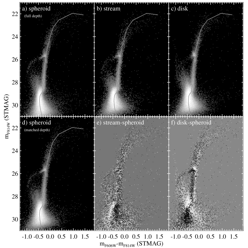
Figure 6.— Comparisons of the CMDs for our three fields. The ridge line for NGC 104 (curve) is shown for reference. a) The CMD of the spheroid field, shown at its full depth, at a logarithmic stretch. b) The CMD of the stream field. c) The CMD of the disk field. d) The CMD of the spheroid field, shown at a depth that matches that in the stream and disk. e) The difference between the stream and spheroid CMDs (with the latter scaled to match the number of stars in the former). The RGB and HB distributions are very similar, but the locus of stars at the MS extends slightly brighter and bluer than that in the spheroid. f) The difference between the disk and spheroid CMDs (with the latter scaled to match the number of stars in the former). The RGB of the disk is considerably redder than that of the spheroid, indicating higher metallicities in the disk. The HB of the disk is almost entirely in the red clump, with a spread to brighter luminosities, indicating higher metallicities and younger ages in the disk. The blue plume of stars above the MSTO is much stronger in the disk, indicating younger ages than in the spheroid.

In a field population, it is difficult to distinguish between young metal-poor stars and old blue stragglers (see Carney, Latham, & Laird 2005 and references therein). Thus, some of the apparently young stars in our CMDs ($\lesssim 6$ Gyr) might instead be blue stragglers. However, whether blue stragglers form via merger or mass transfer, in an old population they will be limited to $M\lesssim$2 $M_{\odot}$. All three of our fields show blue plume stars as bright as the HB over a wide range of color, and in the disk these stars continue to luminosities significantly brighter than the HB. The high masses required to explain the brightest stars in the blue plume population imply that truly young stars are present, and these stars appear to be a smooth extension of the fainter blue plume population. This argues against a significant contribution from blue stragglers in the blue plume.

If we fit Gaussian distributions to the velocity data in our fields (Figure 2), we find that the spheroid is a $\sim$25% contamination in our stream field and a $\sim$33% contamination in our disk field. Given the wide separation between our fields (Figure 1), we cannot necessarily assume that the population in our spheroid field is representative of the spheroid contamination in our stream and disk fields. However, it is natural to ask how the stream and disk CMDs would look if the spheroid contamination were subtracted under the assumption that the population in our spheroid field is in fact representative of this contamination. To show this, we used that subset of the spheroid data that is matched to the depth of the stream and disk data. We randomly drew a star from these spheroid data, found the star in the stream data that most closely agreed in its photometry, and then subtracted that star from the stream data. These subtractions were repeated until 25% of the stream stars were removed. In 99% of the subtractions, the star subtracted from the stream data was within 0.02 mag of the spheroid star, and in 99.9% of the subtractions, the star subtracted from the stream data was within 0.1 mag of the spheroid star; the handful of stars that could not be matched at this level fell very far from the dominant stellar locus (in the negligible cloud of sparse stars at random colors and magnitudes), and these were not subtracted. We repeated this process on the disk data, but there subtracted 33% of the disk stars; again, 99% of the subtractions matched disk to spheroid stars within 0.02 mag, while 99.9% of the subtractions matched disk to spheroid stars within 0.1 mag. The resulting CMDs are shown in Figure 7. Because of the many similarities between the original three CMDs (Figure 2), the changes due to the subtraction of the spheroid contamination are subtle. To help highlight the differences between the three fields, we also show luminosity and color cuts across the CMDs (colored boxes); panels $d$ and $e$ show the color distributions on the lower RGB and HB, respectively, while panels $f$ and $g$ show the luminosity distributions at the red clump and SGB, respectively. The color and luminosity cuts help quantify the similarities and differences between the populations discussed above and shown in Figure 6. Compared to the spheroid population, the stream population exhibits similar RGB and HB morphologies, but its main sequence extends somewhat brighter and bluer. In contrast, the disk population exhibits RGB and HB morphologies that are skewed toward redder colors, with the main sequence showing a strong extension to brighter and bluer colors.

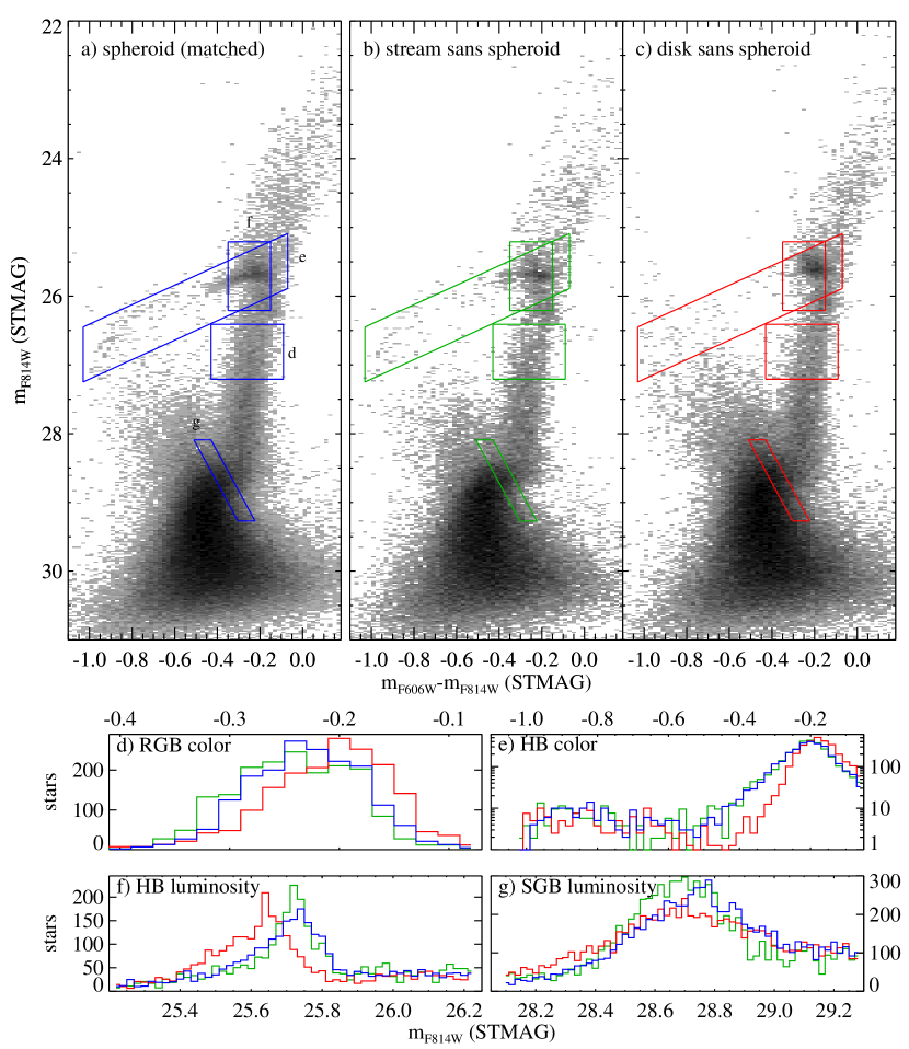
Figure 7.— The spheroid CMD compared to the stream and disk CMDs, where we have attempted to subtract the spheroid contamination from the stream and disk. a) The CMD of the spheroid field, shown at a depth that matches that in the stream and disk fields. Cuts across the CMD (blue boxes) are used to make comparisons with the stream and disk; the histograms in each cut (panels d-g) are normalized to the number of stars in the spheroid. Labels refer to subsequent panels in this figure. b) The CMD of the stream field, with a subtraction of spheroid stars assumed to contaminate at the 25% level, and with the same cuts indicated (green boxes). c) The CMD of the disk field, with a subtraction of spheroid stars assumed to contaminate at the 33% level, and with the same cuts indicated (red boxes). d) Histograms for stars along the RGB color cut for the spheroid (blue), stream (green) and disk (red). e) Histograms along the HB color cut. f) Histograms along the HB luminosity cut. g) Histograms along the SGB luminosity cut. Compared to the spheroid and stream, the disk population has a redder RGB (indicating higher metallicities), an HB that falls mostly in a red clump that extends to brighter luminosities (indicating younger ages and higher metallicities), and a stronger blue plume above the MSTO (indicating younger ages).

5.2. Maximum Likelihood Fitting of Isochrones

We turn now to the quantitative fitting of our CMDs. Our characterization of the star formation history in each field primarily uses the StarFish code of Harris & Zaritsky (2001). This code takes a grid of isochrones, populates them according to the initial mass function (IMF), then applies the photometric scatter and incompleteness (as a function of magnitude and color) determined in the artificial star tests. The code then fits the observed CMD by employing linear combinations of the scattered isochrones. The fitting can be done via minimization of either a $\chi^{2}$ statistic or the Maximum Likelihood statistic of Dolphin (2002). We found little difference between fits done with either statistic, and ultimately used the Maximum Likelihood statistic in our analysis.

In the StarFish fitting, each isochrone at a given age and metallicity is varied independently, resulting in a large number of free parameters in the fit. This method is similar to most of the star formation history methods used in the literature (e.g., Dolphin 2002; Skillman et al. 2003). Although the term “star formation history” might imply a physical connection between the subpopulations, this method is really a fit to the age and metallicity distributions. In addition to StarFish, we wrote our own codes that fit the isochrones to the data according to mathematical and physical restrictions that greatly reduce the number of free parameters; these models will be the subject of a future paper.

We do not fit the entire range of stars observed in the CMD. Instead, we restrict our fits to the lower RGB (below the level of the HB), SGB, and upper main sequence. Specifically, we fit over $-0.9\leq m_{F606W}-m_{F814W}\leq-0.1$ mag in color, and $26.5\leq m_{F814W}\leq 30.5$ mag in magnitude for the spheroid data and $26.5\leq m_{F814W}\leq 30.0$ mag in magnitude for the stream and disk data (which are $\approx$0.5 mag shallower). This region of the CMD offers excellent sensitivity to age and metallicity while avoiding those regions of the CMD that have low signal-to-noise ratio or that are poorly constrained by the models (such as the HB, the upper RGB, the RGB luminosity function bump, and the faint end of the CMD). The HB is a qualitative indicator of age and metallicity, becoming redder at younger ages and higher metallicities, and eventually forming a red clump with a significant spread in luminosity. However, disentangling the effects of age and metallicity is highly uncertain; indeed, the “second parameter debate” in the study of HB morphology refers to the dependence of the HB morphology on parameters other than metallicity, such as age and helium abundance. Although Galactic foreground stars comprise much less than 1% of the stars in our field, they tend to fall near the upper RGB in M31, which is sparsely populated in our data; the upper RGB is thus the one region of our CMDs with significant foreground dwarf contamination. In addition, the upper RGB is contaminated by asymptotic giant branch (AGB) stars, which in turn have a distribution depending on the age and [Fe/H] of their progenitor HB stars. The RGB luminosity function bump is a qualitative metallicity indicator, and it is most prominent in CMDs of metal-rich populations, where it appears as an overdensity on the RGB immediately below the luminosity of the HB; theoretical models reproduce the general trend for the bump luminosity to brighten with decreasing metallicity, but the zeropoint of the relationship is uncertain, and the mix of age and metallicity in our populations makes it difficult to interpret this feature in the data. The faintest main sequence stars in the CMD suffer from large photometric scatter and low completeness.

We use the Victoria-Regina Isochrones (VandenBerg et al. 2006) in all of our fitting. These isochrones do not include core He diffusion, which would decrease their ages at a given turnoff luminosity by $\sim 10$% (VandenBerg et al. 2002). Although the ages of isochrones with core He diffusion are likely more accurate, models in which diffusion is allowed to act efficiently on other elements in the surface layers show significant discrepancies when compared to observed CMDs, indicating that there must be some other mechanism at work, such as turbulence in the surface layers (see Brown et al. 2005 and references therein). Helium diffusion can still occur in the core, and thus the ages discussed herein should be reduced by $\sim$10% to obtain absolute ages.

The Victoria-Regina Isochrones are distributed with a ground-based magnitude system. Sirianni et al. (2005) provide an iterative transformation to put ACS data in a ground-based system, but warn against its use, given the systematic errors intrinsic to such a process. The biggest problem is that the F606W bandpass is very different from Johnson $V$, although the difference between F814W and Cousins $I$ is nonnegligible, too. To properly make the transformation from one system to the other, one must know the intrinsic spectral energy distribution of the source, and this is difficult to estimate based on photometry in two broad bandpasses. It is much more straightforward to use the physical parameters along each model isochrone (effective temperature and surface gravity) to transform the models into the observational system using synthetic spectra of the appropriate metallicity. We use the transformation of Brown et al. (2005), which produces good agreement between these isochrones and the ACS observations of Galactic clusters spanning a wide range in metallicity (Table 2). Over most of the CMD (including the region we use here for fitting), the agreement is better than $\sim$0.02 mag. In this sense, we are using the isochrones to provide relative changes in age and metallicity, once they have been anchored to observations of Galactic clusters. We are thus providing star formation histories in a reference frame based on the ages and metallicities of the clusters listed in Table 2.

5.2.1 The Isochrone Grid

We fit a large grid of isochrones spanning $1\leq$ age $\leq 14$ Gyr (with 0.5 Gyr steps) and $-2.3\leq$ [Fe/H] $\leq+0.5$ (with $\approx$0.1 dex steps) using the StarFish code. The fine spacing in age and metallicity avoids artificial lumpiness in the synthetic CMDs but means that neighboring isochrones in the grid are nearly degenerate. Such degeneracies, plus the large number of free parameters, do not allow a fit to converge in a reasonable time. Fortunately, the StarFish code allows groups of neighboring isochrones to be locked such that their amplitudes vary together; one of these isochrone groups is treated as a single isochrone as far as the fitting is concerned, even if its stars span a small range in age and metallicity (see Harris & Zaritsky 2001 for details). We locked our full grid of isochrones into 117 independent isochrone groups, with the sampling chosen to match the nonlinear changes in the CMD with age and metallicity (the CMD changes more rapidly at higher metallicities and younger ages). The grid of isochrones and the locked isochrone groups are shown in Figure 8.

Figure 8.— The isochrones used in StarFish fitting. A fine grid of isochrones (crosses) was used to avoid artificial lumpiness in the synthetic CMD, but these isochrones were locked together in groups (boxes) to reduce the number of free parameters and to avoid degeneracies in the fit.

5.2.2 Fixed Parameters

Besides distance and reddening, there are several other parameters that must be fixed before proceeding with a fit. The binary fraction is highly uncertain, and not even well-constrained in the field or cluster populations of our own Galaxy; the value appears to be in the range of 10–30% in the field population of the Galactic halo (Ryan 1992 and references therein). The fits to our data are best when the binary fraction is near 10%, whereas fits with the binary fraction significantly deviating from 10% show noticeable residuals. Thus, unless specified otherwise, the binary fraction is assumed to be 10% throughout this paper. The binary fraction is set in the StarFish code (Harris & Zaritsky 2001) at the stage where it scatters the isochrones; specifically, for a given fraction of stars, it draws a second star randomly from the IMF and produces a single unresolved object with the combined color and magnitude of the two stars. For the IMF index, we chose the Salpeter (1955) value of $-1.35$. For the isochrone abundances, we did not assume a scaled-solar abundance pattern. Instead, we assumed that the alpha elements are enhanced at low metallicity and unenhanced (scaled-solar) at high metallicity; specifically, we assumed [$\alpha$/Fe] = 0.3 at [Fe/H] $\leq-0.7$ and [$\alpha$/Fe] = 0.0 at [Fe/H] $>-0.7$. At the [$\alpha$/Fe] resolution available in our isochrone grid, this trend roughly reproduces that seen in the Galaxy (Pritzl, Venn, & Irwin 2005 and references therein), although bulge populations appear to be enhanced in alpha elements even at high metallicity (McWilliam & Rich 1994; Rich & Origlia 2005). As it turns out, the IMF and alpha-enhancement assumptions make little difference in our results. All of these assumptions (distance, reddening, binary fraction, IMF, and alpha enhancement) are varied in our exploration of systematic errors (see §5.6).

5.2.3 Uncertainties

In the fits below, we do not plot error bars for the weights of the individual isochrones. This is because the uncertainty associated with the normalization of any individual isochrone is very large, and correlated with the normalization of neighboring isochrones. If any one isochrone in the best-fit model is deleted from the fit, compensating changes can be made in neighboring isochrones that restore the quality of the fit. The result is that the uncertainty on any individual isochrone weight is largely meaningless. These difficulties are a continuing plague for studies of star formation histories in complex populations (e.g., Skillman et al. 2003; Harris & Zaritsky 2004). If one is fitting a simple stellar population (single age and single metallicity), one can trace out confidence contours in the age-metallicity plane according to the change in fit quality, but with a complex star formation history, it is the distribution of ages and metallicities that matters. What one really wants is a set of isochrones that are truly eigenfunctions of an orthogonal basis set. However, there is not an obvious basis function that relates in a simple way back to physical parameters. The sampling in our isochrone grid is fine enough to avoid artificial structure in the synthetic CMDs, yet coarse enough to avoid isochrones that are completely degenerate within the photometric errors.

Even though some of the isochrone weights in the final fits are very small, the ensemble of these small weights is necessary for a good fit. One way of demonstrating this assertion is by repeating the fits after deleting isochrones with low weights. Starting with the best fit, we first sorted the isochrones by their fitted weights, and then retained only those whose weight exceeded a specified cutoff; specifically, the cutoff in weight was chosen so that this subset of isochrones accounted for 90% of the stars in the best fit. Refitting with this reduced set of isochrones produced terrible fits (fit score $\sim$50% larger). The fit was also poor when we retained those isochrones responsible for 95% of the stars in the best fit. The fit did not become acceptable until we had retained those isochrones responsible for 99% of the stars in the best fit ($\sim$50 of the original 117 isochrone groups).

5.3. Results for the Spheroid

The distribution of age and metallicity in our best fit to the spheroid data is shown in Figure 9. In this figure, the area of the symbols (filled circles) is proportional to the number of stars in each isochrone group. Note that the spacing of the isochrone groups is irregular, so that if one were to plot a star formation rate in units of $M_{\odot}$ per unit time per unit logarithmic metallicity, the relative sizes of the symbols would be somewhat increased at younger ages and higher metallicities (where the spacing is finer). As noted by Brown et al. (2003), the spheroid CMD is best fitted by a wide range of age and metallicity, and is strikingly different from the old, metal-poor halo of the Milky Way. Approximately 40% of the stars are less than 10 Gyr old, and approximately 50% of the stars are more metal-rich than 47 Tuc ([Fe/H]$\approx-0.7$). The mean metallicity, $<$[Fe/H]$>$=$-0.6$, is identical to that found by Durrell et al. (1994) at 9 kpc on the minor axis, and slighter higher than the $<$[m/H]$>$=$-0.6$ found by Holland et al. (1996) from earlier WFPC2 photometry of our field, with similar spreads to both higher and lower metallicities. Although our mean metallicity is much higher than that in the Milky Way halo, the metallicity distribution definitely has a tail extending to metal-poor stars. These include the RR Lyrae stars in our field, which have a mean metallicity of [Fe/H] = $-1.7$ (Brown et al. 2004a), and the minority population of blue HB stars.

Figure 9.— The distribution of age and metallicity in the best-fit model of the spheroid data. The area of the filled circles is proportional to the number of stars in each isochrone group.

Although we used the Dolphin (2002) Maximum Likelihood statistic to perform our fits, we also compared the results with those obtained from a traditional $\chi^{2}$ statistic, and the fits were similar. Dolphin (2002) also provides a goodness of fit statistic, $\chi^{2}_{\rm eff}$, for those more familiar with $\chi^{2}$ fitting (with values close to unity indicating a good fit). The best fit model (Figure 9) has $\chi^{2}_{\rm eff}=1.11$ per degree of freedom (8000 CMD bins minus 117 freely varying isochrone weights). This score clearly implies an imperfect fit. To demonstrate this, we ran Monte Carlo simulations of the idealized case. We created random realizations of the data drawn from the best-fit model to obtain the distribution of the Maximum Likelihood statistic, and found that the Maximum Likelihood statistic obtained in our best-fit model exceeds the mean score by 6$\sigma$ (where $\sigma$ is one standard deviation in the distribution of the Maximum Likelihood statistic from the Monte Carlo runs).

There are many reasons why the model should not exactly reproduce the data. These include imperfections in the isochrones (they are calibrated at the $\sim$0.02 mag level against Galactic globular clusters observed in the same filters), deviations from a Salpeter (1955) IMF, deviation from our assumed binary fraction of 10% (e.g., one might imagine that the binary fraction varies with age and metallicity depending on the variations in the formation environment), and the limitations of the artificial star tests used to scatter the isochrones (artificial stars are created, with noise, from the same PSF model used in the PSF fitting, while real stars will deviate from the PSF model due to noise and true intrinsic inaccuracies in the PSF model). Although the model does not exactly reproduce the data distribution over 8000 CMD bins, the deviations are remarkably small, as we show in Figure 10. In the top row of panels, we show the data in the fitting region (yellow), the best-fit model (blue), and the differences between the two (yellow and blue) shown at the same linear stretch; i.e., the CMD bins in panel $c$ are shaded blue where the model exceeds the data, and shaded yellow where the data exceeds the model, with the shading on the same linear scale employed in panels $a$ and $b$. The differences between the data and model appear almost completely random, with minimal systematic residuals; in fact, the upper panels look much like the idealized case shown in the bottom row of panels, where the residuals are completely random. There, we show a random realization of the best-fit model (yellow), a repeat of the best-fit model (blue), and the differences between the two (yellow and blue). The realization (bottom left) is nearly indistinguishable from the actual data (top left). The difference between the realization and the model (bottom right) demonstrates the noise residuals one can expect when comparing a smooth model to discrete data in the idealized case ($\chi^{2}_{\rm eff}=1$).

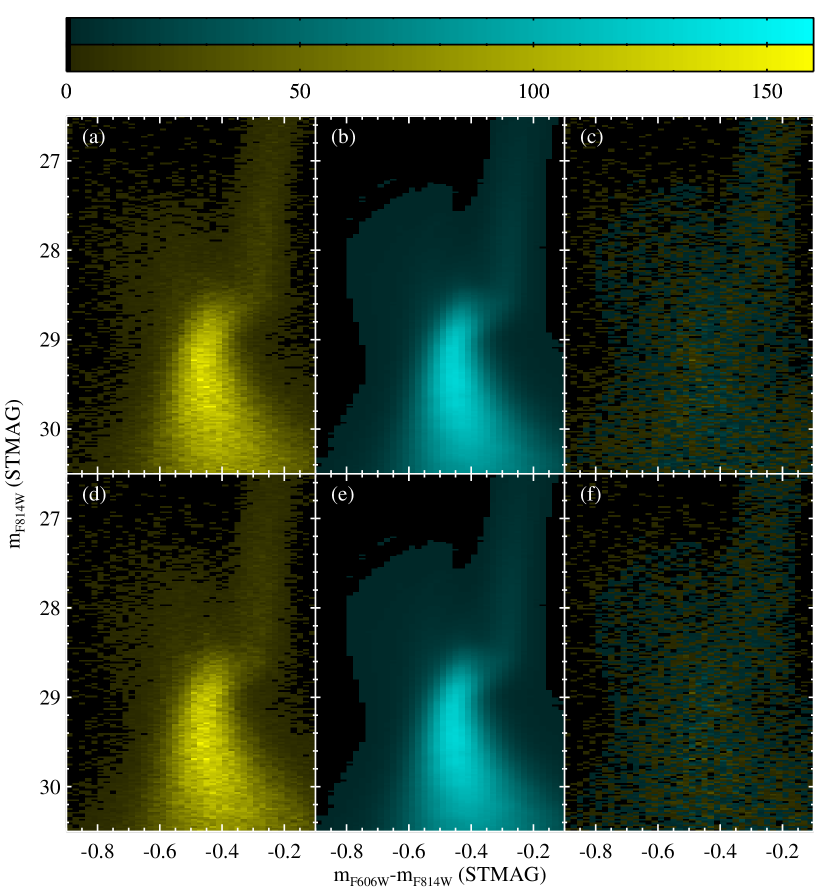
Figure 10.— Top panels: The CMD of the spheroid data (yellow), the best-fit model to those data (blue), and the differences between the data and model (yellow and blue), all shown at the same linear stretch. Bottom panels: An artificial CMD drawn from the best-fit model (yellow), the same best-fit model (blue), and the differences between the artificial data and model (yellow and blue), all shown at the same linear stretch employed in the top panels.

Given the large number of free parameters, one might also wonder if the “best-fit” model has truly converged on the best fit. One way to test this is through repeated fitting with distinct initial conditions. We show in Figure 11 the results of three “best-fit” models to the spheroid data, each of which started from a distinct random set of isochrone weights. Although there are small variations in the final individual isochrone weights, it is clear that the overarching result is the same in each case. As stated earlier, the degeneracies in the isochrone set mean that any individual isochrone can be varied significantly without changing the fit quality. For example, in Figure 11, the relatively low weight at [Fe/H]=$-1.7$, compared to the weights at [Fe/H]=$-1.4$ and [Fe/H]=$-2.1$, is not meaningful; for the isochrones at 13 Gyr, we can redistribute the weights at [Fe/H]=$-1.4$, $-1.7$, and $-2.1$ so that they are the same in each of these bins, and the fit quality does not suffer.

Figure 11.— Three different attempts at fitting the spheroid data, using the same isochrones in each case, but where the initial guess in each panel was a distinct random distribution of isochrones. The area of the filled circles is proportional to the number of stars in each isochrone group. Although there are small variations in the individual amplitude weights from panel to panel, it is clear that the best-fit model is well converged.

Although the uncertainties on the individual isochrone weights in the best-fit model are large, one can ask what classes of models, in a broad sense, produce fits that are as good as the best-fit model. If one restricts the fit to isochrones of ages$<10$ Gyr, the quality of the fit is noticeably reduced, with $\chi^{2}_{\rm eff}=1.18$ (a fit that is an additional 5$\sigma$ worse than the best-fit model). Much of the weight in this fit falls at the top end of the allowed age range, and the difference between the model CMD and the data CMD shows significant residuals (Figure 12). Alternatively, if one restricts the fit to isochrones with ages$\geq 10$ Gyr, the quality of the fit is grossly reduced, with $\chi^{2}_{\rm eff}=3.09$ and very obvious differences between the model CMD and the data CMD (Figure 12). This is consistent with the results of Brown et al. (2003), who showed that the spheroid CMD is inconsistent with a purely old population of stars.

Table 3Summary of Spheroid Fitting

Model	$<$[Fe/H]$>$	$<$age$>$	$\chi^{2}_{\rm eff}$	Comment
Standard model	$-0.6$	9.7	1.11	Minimal residuals in fit
Age $<10$ Gyr	$-0.5$	8.4	1.18	Significant residuals in fit
Age $\geq 10$ Gyr	$-0.8$	10.9	3.09	Gross residuals in fit
No old metal-rich stars	$-0.6$	9.6	1.11	Minimal residuals in fit
No young metal-poor stars	$-0.6$	9.7	1.18	Misses part of plume

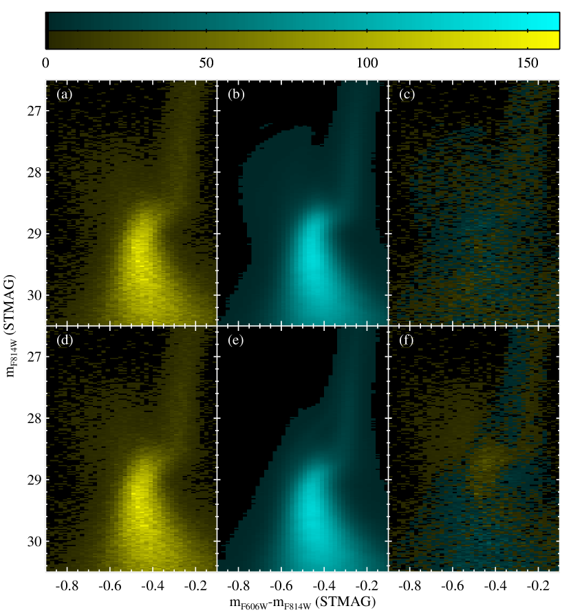
Figure 12.— Top panels: The CMD of the spheroid data (yellow), the best-fit model to those data using a set of isochrones restricted to ages less than 10 Gyr (blue), and the differences between the data and model (yellow and blue), all shown at the same linear stretch. Bottom panels: The same CMD of the spheroid data (yellow), the best-fit model to those data using a set of isochrones restricted to ages $\geq 10$ Gyr (blue), and the differences between the data and model (yellow and blue), all shown at the same linear stretch employed in the top panels. It is clear that neither model is acceptable, given the residuals (right hand panels).

The best-fit model has minority populations in the isochrones representing old metal-rich stars and young metal-poor stars. If truly present, these populations are extremely interesting, because the former imply that at least some of the stars were formed in something like a bulge environment (with rapid early enrichment), while the latter imply the accretion of metal-poor stars from dwarf galaxies or star formation following the infall of relatively pristine material. To test this, we repeated the fit while excluding two regions from the input grid of isochrones: age$\geq 10$ Gyr at [Fe/H]$\geq 0$, and age$<5$ Gyr at [Fe/H]$<-0.5$; each of these regions contains 3% of the stellar mass in the best-fit model. If the old metal-rich isochrones are excluded from the fit, the fit quality in the resulting model does not suffer at all; thus, the CMD is consistent with either a small population of such old metal-rich stars or none at all. In contrast, if the young metal-poor isochrones are excluded from the fit, the fit quality is somewhat reduced, with $\chi^{2}_{\rm eff}=1.18$, due to the model missing the brightest and bluest stars in the blue plume above the dominant main sequence. This is not surprising, given our visual inspection of the CMD and comparison to young isochrones of various metallicities (Figure 4). Note that the scattered model isochrones include the effects of blends (determined by the artificial star tests) but not any contribution from blue stragglers; thus, some (but not all) of the young stars in the fit ($\lesssim 6$ Gyr) could be an attempt to account for blue stragglers (see §5.1).

We summarize the fits to the spheroid data in Table 3. Our standard model is that which simply allows the full grid (Figure 8) to vary freely, while the other models are self-explanatory. Mean values of [Fe/H] and age are not as useful as the full age and metallicity distributions, given the complicated star formation history present in the field, but these mean values do serve as a yardstick to gauge differences between the fits.

5.4. Results for the Stream

The distribution of age and metallicity in our best fit to the stream data is shown in Figure 13. Given the qualitative similarities between the stream and spheroid CMDs, it is not surprising that the best-fit distribution of age and metallicity in the stream resembles that in the spheroid. However, as noted above, there are some distinctions. The mean age in the stream (8.8 Gyr) is $\sim$1 Gyr younger than that in the spheroid (9.7 Gyr), while the mean metallicities are nearly the same ($-0.6$ in the spheroid and $-0.7$ in the stream). The fit quality for the best-fit stream model is similar to that for the spheroid, with $\chi^{2}_{\rm eff}=1.08$. In Figure 14, we show the comparison of the best-fit model to the data, as well as the residuals.

Given that the stream and spheroid are so similar, we also explored to what extent both populations might be consistent with a single star formation history. First, we simply used the spheroid star formation history (Figure 9) to normalize a set of isochrones scattered according to the stream artificial star tests, and then scaled the result to match the number of stars in the stream. This created a model with the spheroid star formation history but the observational properties of the stream data, enabling a fair comparison of the two. The result is shown in Figure 15. It is obvious that there are gross residuals in the model. Although this was not a fit (given that we simply applied the star formation history of the spheroid), if this model had resulted from our standard isochrone fitting, it would have produced a $\chi^{2}_{\rm eff}$ of 1.32. The comparison of the spheroid data with this model population yielded a $\chi^{2}_{\rm eff}$ of 1.11 (§5.3); the much larger discrepancy of the stream data with this model population strongly implies that the spheroid and stream data were drawn from distinct populations, at a confidence level exceeding 99%.

Figure 13.— The distribution of age and metallicity in the best-fit model of the stream data. The area of the filled circles is proportional to the number of stars in each isochrone group. The total area within the filled symbols has been normalized to that in Figure 9, to ease comparison (but in reality the surface brightness in the stream is $\sim$0.5 mag fainter).

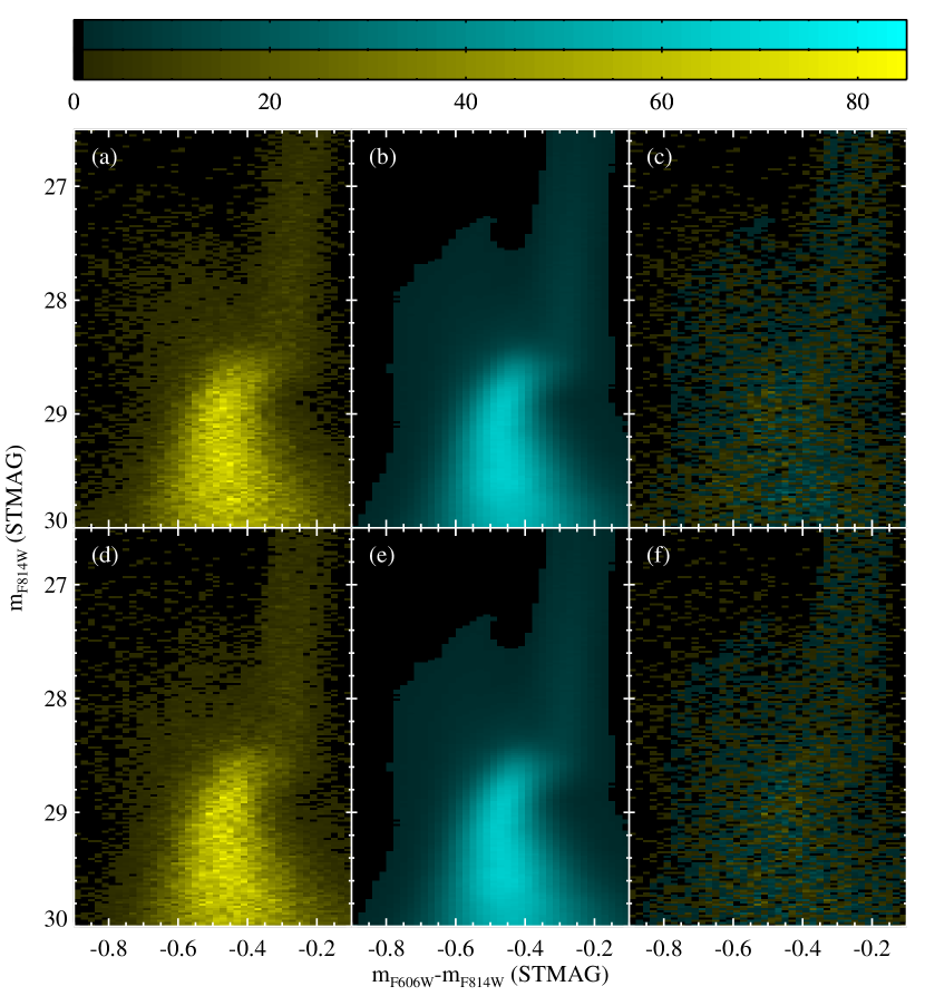
Figure 14.— Top panels: The CMD of the stream data (yellow), the best-fit model to those data (blue), and the differences between the data and model (yellow and blue), all shown at the same linear stretch. Bottom panels: An artificial CMD drawn from the best-fit model (yellow), the same best-fit model (blue), and the differences between the artificial data and model (yellow and blue), all shown at the same linear stretch employed in the top panels. Note that the magnitude range of the stream fit is smaller than that in the spheroid fit, because the spheroid data are $\sim$0.5 mag deeper than the stream data.

Next, we tried fitting both the spheroid and stream simultaneously with the same star formation history. Specifically, a model for the stream was constructed from isochrones appropriately matching the stream observations (utilizing the stream artificial star tests), and a model for the spheroid was constructed from isochrones appropriately matching the spheroid observations (utilizing the spheroid artificial star tests), but the relative weights of the isochrones used to construct these stream and spheroid models came from a single distribution of age and metallicity. This distribution was varied until the best fit to both the stream and spheroid data was achieved. The resulting age and metallicity distribution is shown in Figure 16. Curiously, this compromise solution to both CMDs is a bit older and more metal-poor than that found for either CMD individually; this is likely due to the fact that the spheroid and stream are distinct, resulting in a poor fit when fitting both at the same time. The poor quality of the fit can be seen when this compromise model is compared to the stream data, as shown in Figure 15. The value for $\chi^{2}_{\rm eff}$ is not terrible (1.14), but there are approximately twice the number of degrees of freedom in this fit, given that we are fitting two CMDs of data simultaneously, so the deviation from unity is more significant. Both of these tests imply that while the stream and spheroid CMDs are very similar, they are not drawn from exactly the same population.

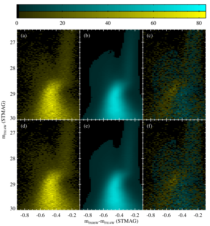
Figure 15.— a) The CMD of the stream data (yellow). b) A model for the stream data (blue), but constructed from the spheroid star formation history, scattered with the observational errors of the stream data and normalized to the stream star counts. c) The differences between the data and model (yellow and blue), all shown at the same linear stretch. d) The same CMD of the stream data (yellow). e) The best-fit compromise model fit simultaneously to the spheroid and stream datasets (blue). f) The differences between the data and model (yellow and blue), all shown at the same linear stretch employed in the top panels. Significant residuals can be seen in either case (right hand panels) implying that the stream and spheroid CMDs are not drawn from the same population.

Figure 16.— The distribution of age and metallicity in the best-fit model simultaneously fit to the spheroid and stream data. The area of the filled circles is proportional to the number of stars in each isochrone group. The distribution shown here is clearly a compromise between those shown in Figures 9 and 13.

As done with the spheroid data, we also explored to what extent stream models with more restricted age ranges are consistent with the data. When the isochrones are restricted to ages$<10$ Gyr, the quality of the fit is nearly unchanged (with $\chi^{2}_{\rm eff}=1.10$), although the resulting distribution of age and metallicity looks somewhat skewed, with much of the weight falling at the top end of the age range. When the isochrones are restricted to ages$\geq 10$ Gyr, the quality of the fit is very poor, with $\chi^{2}_{\rm eff}=2.80$. If old metal-rich stars are removed from the input isochrone grid, the quality of the fit is unchanged from the best fit model, while if young metal-poor stars are removed, the quality of the fit is noticeably affected, with $\chi^{2}_{\rm eff}=1.14$, but the model is only missing the brightest and bluest stars in the blue plume.

Table 4Summary of Stream Fitting

Model	$<$[Fe/H]$>$	$<$age$>$	$\chi^{2}_{\rm eff}$	Comment
Standard model	$-0.7$	8.8	1.08	Minimal residuals in fit
Age $<10$ Gyr	$-0.6$	8.1	1.10	Minimal residuals in fit
Age $\geq 10$ Gyr	$-1.0$	11.0	2.80	Gross residuals in fit
No old metal-rich stars	$-0.7$	8.8	1.09	Minimal residuals in fit
No young metal-poor stars	$-0.7$	8.8	1.14	Misses part of plume
Best-fit spheroid model	$-0.6$	9.7	1.32	Gross residuals
Simultaneous fit to spheroid stream	$-0.8$	10.1	1.14	Significant residuals
Fixed 25% spheroid contamination	$-0.8$	8.8	1.10	Similar to standard model
aNot actually a fit. See text for details.
bTwice the degrees of freedom. See text for details.

The Keck data for our stream field imply that 75% of its stars fall in two kinematically cold stream components (Kalirai et al. 2006b), and that 25% of its stars are in the underlying spheroid. Although the population in our spheroid field might not be representative of the underlying spheroid in the stream field, it is reasonable to wonder how the fitting of the stream star formation history is affected if this spheroid contamination is taken into account. To explore this, we fitted the stream with the same set of isochrones, but added an additional component to the model, fixed at 25% of the population, representing the spheroid contamination. This contamination component was constructed from the best-fit model to the spheroid but using the isochrones scattered with the stream artificial star tests; thus the contamination component appropriately represents the spheroid population as it would appear in the stream data. The results are shown in Figure 17. The quality of the fit is good; $\chi^{2}_{\rm eff}=1.10$. In the top panel, we show the total star formation history (combining the fixed spheroid contamination and the fit to the stream). In the bottom panel, we have subtracted the spheroid contamination component from the star formation history, to show the star formation history of the stream in isolation. The isolated star formation history of the stream (Figure 17b) is very similar to the best-fit model to the stream that did not try to account for the spheroid contamination (Figure 13). Given the similarity between the stream and spheroid CMDs, and the fact that the spheroid contamination is only 25%, this is not that surprising. We summarize the results of the stream fitting in Table 4.

Figure 17.— The best-fit model to the stream, assuming a fixed 25% contamination from the underlying spheroid that matches the population in Figure 9. The area of the filled circles is proportional to the number of stars in each isochrone group. Top panel: The complete star formation history, including the fixed spheroid contamination. Bottom panel: The star formation history for the stream population in isolation, excluding that part of the fit representing the spheroid contamination. The population has been normalized such that the total area in the symbols is the same in both panels.

5.5. Results for the Disk

The distribution of age and metallicity in our best fit to the disk data is shown in Figure 18. As expected from our earlier inspection of the CMDs, the star formation history in the disk is markedly distinct from that in the spheroid or stream, in the sense that the population is younger and significantly more metal-rich, with a mean age of 7.5 Gyr and a mean metallicity of [Fe/H] = $-0.2$. The fit quality for the best-fit disk model is excellent, with $\chi^{2}_{\rm eff}=1.05$. In Figure 19, we show the comparison of the best-fit model to the data, as well as the residuals.

Figure 18.— The distribution of age and metallicity in the best-fit model of the disk data. The area of the filled circles is proportional to the number of stars in that isochrone group. The distribution shown here is clearly distinct from those shown in Figures 9 and 13. The total area within the filled symbols has been normalized to that in Figures 9 and 13, to ease comparisons.

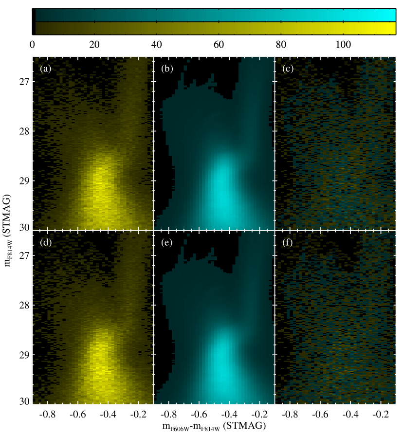
Figure 19.— Top panels: The CMD of the disk data (yellow), the best-fit model to those data (blue), and the differences between the data and model (yellow and blue), all shown at the same linear stretch. Bottom panels: An artificial CMD drawn from the best-fit model (yellow), the same best-fit model (blue), and the differences between the data and model (yellow and blue), all shown at the same linear stretch employed in the top panels. Note that the magnitude range of the disk fit is smaller than that in the spheroid fit, because the spheroid data are $\sim$0.5 mag deeper than the disk data.

The best-fit model to the disk is dominated by stars at ages of less than 10 Gyr. In fact, if we fit the data with a subset of the isochrones restricted to ages$<$10 Gyr (i.e., remove all old isochrones from the input grid, not just the metal-rich ones), the fit is only negligibly worse than that achieved with the full set of isochrones ($\chi^{2}_{\rm eff}=1.06$), and the resulting distribution of age and metallicity looks very similar to that in the best-fit model. In contrast, a fit restricted to ages$\geq 10$ Gyr is grossly inadequate, with $\chi^{2}_{\rm eff}=5.07$. If young metal-poor stars are removed from the fit (as done with the stream and spheroid fitting), the fit quality drops, with $\chi^{2}_{\rm eff}=1.14$, and the model misses the bright blue stars in the plume.

Table 5Summary of Disk Fitting

Model	$<$[Fe/H]$>$	$<$age$>$	$\chi^{2}_{\rm eff}$	Comment
Standard model	$-0.2$	7.5	1.05	Minimal residuals in fit
Age $<10$ Gyr	$-0.1$	6.9	1.06	Minimal residuals in fit
Age $\geq 10$ Gyr	$-0.9$	11.0	5.07	Gross residuals in fit
No young metal-poor stars	$-0.2$	7.6	1.14	Misses part of plume
Fixed 33% spheroid contamination	$+0.1$	6.6	1.05	Younger. Minimal residuals

The metallicity distribution in our best fit to the disk CMD is somewhat more metal-rich than that typically found in the outer disk of M31 (e.g., Worthey et al. 2005). There are several possible reasons for this. First, the greatest color dependence upon [Fe/H] is at the tip of the RGB, which in our data is both sparsely populated and seriously contaminated by foreground dwarf stars. Instead, we are using the lower RGB, which offers the advantage of large numbers of M31 stars and little contamination, but the penalty is a reduced color sensitivity to [Fe/H]. Second, the use of distinct isochrone sets and distinct observing bands results in significant scatter for abundance determinations even when the population is a simple one, such as a globular cluster. The metallicities we derive are calibrated to the globular cluster metallicities given in Table 2. Published abundances for globular clusters of intermediate metallicity vary by $\sim$0.2 dex in the recent literature, while abundances for high metallicity clusters vary by even more (see Brown et al. 2005 and references therein). Moreover, isochrones at high metallicity are difficult to calibrate, given that appropriate clusters tend to be in heavily reddened regions, such as the Galactic bulge. Finally, previous [Fe/H] distributions for M31 fields invariably employed old isochrones or the ridge lines of old globular clusters as reference points. This will bias the results toward lower metallicity if the metal-rich population is in fact significantly younger than Galactic globular clusters. For example, the upper RGB for a 13 Gyr population at [Fe/H] = 0.0 is very similar to that for a 6 Gyr population at [Fe/H] = +0.230.

The Keck kinematics of our disk field imply that $\sim$67% of its stars are moving in the disk (Kalirai et al. 2006b; Reitzel et al. in prep.), and that $\sim$33% of its stars are in the underlying spheroid. As with our analysis of the stream, the population in our spheroid field might not be representative of the underlying spheroid in the disk field, but it is reasonable to explore a fit to the disk with a fixed contamination component from the spheroid. We repeated the disk fitting with an additional model component held fixed at 33% of the population, representing spheroid contamination. This contamination component was constructed from the best-fit model to the spheroid but using the isochrones scattered with the disk artificial star tests; thus the contamination component appropriately represents the spheroid population as it would appear in the disk data. The results are shown in Figure 20. The quality of the fit is excellent, with $\chi^{2}_{\rm eff}=1.05$. In the top panel, we show the total star formation history (which includes the fixed spheroid component in the fit to the disk field). In the bottom panel, we show the same fit to the star formation history, but subtract that fixed component representing spheroid contamination, in order to show the star formation history of the disk population in isolation. The isolated disk population (Figure 20b) is significantly younger and more metal-rich than that found in our initial model (Figure 18), where we did not try to account for the spheroid contamination. The isolated point at 13 Gyr and [Fe/H] = 0.5 is not significant (repeating the fit with no isochrones older than 10 Gyr yields $\chi^{2}_{\rm eff}=1.06$). The similarities between Figures 18 and Figure 20a are reassuring; the fit in Figure 18 did not employ any knowledge of the spheroid contamination, yet it is clear that this fit tried to reproduce the old metal-poor component that is present in Figure 20a, where we explicitly specified a spheroid contamination component to the model. Because the spheroid contamination can completely account for the old and metal-poor stars in the disk field, the dearth of metal-poor stars is another example of the “G dwarf problem” – that a simple closed box model of chemical evolution predicts a longer tail of metal-poor stars than seen in all massive galaxies (see Worthey et al. 2005 and references therein). We summarize the results of the disk fitting in Table 5.

Figure 20.— The best-fit model to the disk, assuming a fixed 33% contamination from the underlying spheroid that matches the population in Figure 9. Top panel: The complete star formation history, including the fixed spheroid contamination. Bottom panel: The star formation history for the disk population in isolation, excluding that part of the fit representing the spheroid contamination. The population has been normalized such that the total area in the symbols is the same in both panels.

5.6. Systematic Effects of Binaries, Alpha-enhancement, IMF, Distance, and Reddening

The fits above make assumptions about the binary fraction, alpha-element enhancement, IMF, distance, and reddening. Of these three parameters, the binary fraction and reddening uncertainties translate into the largest uncertainties in the resulting fits, but do not change the gross interpretation of the CMDs. We assumed an IMF index of $-1.35$ (Salpeter 1955), and assumed that [$\alpha$/Fe] = 0.3 at [Fe/H] $\leq-0.7$ and [$\alpha$/Fe] = 0.0 at [Fe/H] $>-0.7$. We assumed 770 kpc for the M31 distance (Freedman & Madore 1990), which is based on Cepheids and falls in the middle of the range generally quoted in the literature (e.g., Pritchet & van den Bergh 1987; Stanek & Garnavic 1998; Holland 1998; Durrell et al. 2001; McConnachie et al. 2005; Ribas et al. 2005). We assumed $E(B-V)=0.08$ mag in each field, but as noted earlier, the Schlegel et al. (1998) map is uncertain at the $\sim$0.02 mag level in random fields, with somewhat higher uncertainties near Local Group galaxies.

We chose a binary fraction of 10%, because grossly changing this value produced lower quality fits with obvious residuals in the comparison of the models and data. Given that we chose a binary fraction that minimized fit residuals, in a sense we “fit” the binary fraction, but did so on a very coarse scale. Fortunately all three fields can be reasonably fit with the same binary fraction, because this avoids complications in the interpretation of the fits. If we assumed distinct binary fractions in the fitting to each field, one could attribute some of the age variations to this varying binary fraction. At larger binary fractions, the features in the synthetic CMD become brighter, and the age distribution must shift to older ages to compensate, while lower binary fractions result in younger age distributions.

To demonstrate the sensitivity of our fits to these parameters, we repeated our fits while varying our assumptions. The results are shown in Table 6 for all three fields, and in Figure 21 for the spheroid field. Reducing the binary fraction to 0% would decrease our ages by 0–0.4 Gyr, while increasing the binary fraction to 40% would increase our ages by $\sim$1 Gyr. Changing the alpha enhancement has almost no effect, other than a slight shift in the metallicity distribution. The insensitivity to alpha enhancement makes sense, because in these bandpasses, isochrones with enhanced alpha elements look much like scaled-solar isochrones at slightly higher metallicity (note that the isochrones are always transformed to the ACS bandpasses using synthetic spectra of a consistent alpha enhancement; see Brown et al. 2005). Changing the IMF index from $-1.35$ to $-1.15$ also has little effect on the metallicity and age distributions; this is because our CMDs are sampling a fairly small range in stellar mass (the bulk of the stars brighter than the faint limit in our fitting region fall in the mass range 0.7$\lesssim M\lesssim 1.2$ $M_{\odot}$). Changing the extinction by 0.03 mag in either direction (assuming the average Galactic extinction curve of Fitzpatrick 1999) primarily affects the metallicity distribution; an increase in the assumed extinction (redder stars) is compensated by a lower metallicity (bluer stars), and vice versa. Changing the distance modulus by 0.03 mag in either direction primarily affects the age distribution; an increase in the assumed distance (fainter apparent magnitudes) is compensated by a younger age (brighter absolute and apparent magnitudes), and vice versa. Note that no change in assumptions for the spheroid (Figure 21) can make the spheroid population look like that of the disk (Figure 18).

Table 6Systematic Effects of Assumptions

	spheroid			stream			disk
Fit	$<$age$>$	$<$[Fe/H]$>$	$\chi^{2}_{\rm eff}$	$<$age$>$	$<$[Fe/H]$>$	$\chi^{2}_{\rm eff}$	$<$age$>$	$<$[Fe/H]$>$	$\chi^{2}_{\rm eff}$
Standard model	9.7	$-$0.6	1.11	8.8	$-$0.7	1.08	7.5	$-$0.2	1.05
Binary fraction = 0.0	9.3	$-$0.5	1.14	8.7	$-$0.7	1.09	7.5	$-$0.1	1.11
Binary fraction = 0.2	10.1	$-$0.8	1.17	9.2	$-$0.8	1.13	7.7	$-$0.2	1.05
Binary fraction = 0.4	10.9	$-$0.9	1.42	9.9	$-$1.0	1.25	8.5	$-$0.4	1.13
$[\alpha$/Fe$]=0.3$ at [Fe/H]$\leq$0	9.7	$-$0.7	1.11	8.9	$-$0.8	1.08	7.7	$-$0.3	1.05
$[\alpha$/Fe$]=0.0$ at all [Fe/H]	9.7	$-$0.6	1.11	8.9	$-$0.7	1.08	7.6	$-$0.1	1.05
IMF index $-$1.15	9.9	$-$0.7	1.11	9.0	$-$0.7	1.08	7.6	$-$0.2	1.04
Distance = 760 kpc	9.8	$-$0.7	1.12	9.1	$-$0.7	1.09	7.6	$-$0.2	1.04
Distance = 780 kpc	9.5	$-$0.6	1.11	8.7	$-$0.7	1.08	7.4	$-$0.1	1.05
$E(B-V)=0.05$ mag	9.8	$-$0.2	1.15	9.1	$-$0.3	1.08	7.7	$+$0.2	1.14
$E(B-V)=0.11$ mag	9.4	$-$1.0	1.17	8.6	$-$1.1	1.16	7.3	$-$0.5	1.05

Figure 21.— The distribution of age and metallicity in the best-fit model to the spheroid data, making different assumptions about the binary fraction, IMF, alpha-enhancement, distance, and reddening. The area of the filled circles is proportional to the number of stars in each isochrone group. a) Our standard model: binary fraction 10%, Salpeter (1955) IMF, alpha-element enhancement at [Fe/H]$<-0.7$, distance of 770 kpc, $E(B-V)=0.08$ mag. b) A binary fraction of 0%. c) A binary fraction of 20%. d) A binary fraction of 40%. e) Isochrones at [Fe/H]$\leq 0$ are alpha-enhanced. f) None of the isochrones are alpha-enhanced. g) An IMF index of $-1.15$. h) Distance is 760 kpc. i) Distance is 780 kpc. j) $E(B-V)=0.05$ mag. k) $E(B-V)=0.11$ mag.

6. Discussion

The quantitative fitting to the CMDs of the spheroid, stream, and outer disk reaffirmed our general impressions from the qualitative inspection of the CMDs. In Figure 22, we compare the star formation histories for the three fields. The star formation history in the spheroid is simply our standard model (Figure 9), while the star formation histories in the stream and disk are those that have had an assumed spheroid contamination subtracted (Figures 17b and 20b). All three fields show an extended star formation history. The star formation history in the stream is similar to that in the spheroid, but is shifted somewhat younger. The disk population is dominated by intermediate-age stars, with little evidence for the old metal-poor population present in the spheroid and stream. All three fields have a trace population of young metal-poor stars, presumably due to the accretion of metal-poor stars from dwarf galaxies or due to stars forming from the infall of relatively pristine material. The fact that such material continues to fall into Andromeda is evidenced by the extensive population of H I clouds recently found in the outskirts of the galaxy (Thilker et al. 2004).

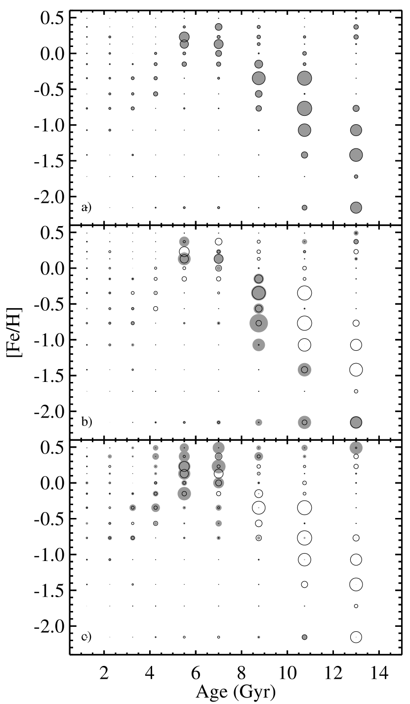
Figure 22.— The best-fit star formation histories for the spheroid ($a$), stream ($b$), and disk ($c$). The area of the filled circles (grey) is proportional to the number of stars falling in the given isochrone. For comparison, the star formation history of the spheroid is overplotted in each panel (black open circles) The stream and disk fits each assumed a fixed contamination from the spheroid, which has been subtracted.

6.1. Disk

Most hierarchical CDM models predict that a spiral disk forms inside-out, generally leading to a disk that becomes progressively younger at increasing radius. For example, the simulated disk of Abadi et al. (2003a, 2003b) has a mean age of $\sim 8$–10 Gyr within 2 kpc of the center and $\sim$6–8 Gyr near 20 kpc. However, the literature does include counter-examples with more complex age gradients. The simulated galaxy of Robertson et al. (2004) exhibits a mean stellar age of $\sim$7.5 Gyr in the center (within 2 kpc) and $\sim$10 Gyr in the disk outskirts (beyond 14 kpc). The CDM models of Sommer-Larson, G$\ddot{\rm o}$tz, & Portinari (2003) result in disk galaxies that sometimes form inside-out and sometimes form outside-in. Both classes predict mean ages of 6–8 Gyr in the outer disk (6 scale lengths from the center), but the age distributions differ, with the inside-out galaxy hosting a significantly larger fraction of young stars ($\lesssim 3$ Gyr) in the outskirts. In a sophisticated model of the chemical evolution in the Milky Way disk, Chiappini et al. (2001) demonstrate an inside-out formation scenario where the stellar age is not a monotonically varying function of distance from the Galactic center; in the inner disk (4–10 kpc), the stellar ages are decreasing with increasing radius, as expected, but beyond this radius, the stellar ages increase with radius, because the thick disk and halo begin to dominate over the thin disk. All of these models can be compared to the solar neighborhood (e.g., Ibukiyama & Arimoto 2002; Sandage, Lubin, & VandenBerg 2003; Fontaine, Brassard, & Bergeron 2001), but we know little of the detailed star formation histories for other giant spiral galaxies. As far as the structures are concerned, observations of high-redshift disk galaxies (e.g. Ferguson, Dickinson & Williams 2000; Ravindranath et al. 2004) suggest that disks were largely in place 8 Gyr ago. Since then, they have increased their stellar masses and increased their sizes consistent with an inside-out sequence of star formation (Trujillo et al. 2005), with the average stellar surface mass density staying roughly constant from $z=1$ to the present (Barden et al. 2005).

Our mean age in the outer disk (6.6 Gyr) is in good agreement with the models of Abadi et al. (2003a, 2003b), and significantly younger than the models of Robertson et al. (2004); these comparisons suggest a consistency with an inside-out formation scenario. Our mean age also falls in the range found in both the inside-out and outside-in models of Sommer-Larson et al. (2003), but our age distribution, with a significant dearth of stars younger than 3 Gyr, is in somewhat better agreement with their outside-in model. However, these are all hydrodynamical models that track the birth of particles but largely ignore the details of chemical evolution. It would be interesting to compare our age-metallicity distribution with such a distribution in a true chemical evolution model under an inside-out formation scenario (e.g., Chiappini et al. 2001).

Our star formation history in the disk is probably saying less about the validity of the inside-out formation scenario and more about the relative scales of the thin and thick disk; because our disk field is 25 kpc from the galactic center, it is well into the regime where one might expect the thick disk to dominate (Chiappini et al. 2001). Indeed, there is evidence that the thick disk begins to dominate well inside this radius; in their WFPC2 images of an off-axis field 5 kpc from the nucleus, Sarajedini & Van Duyne (2001) found a population apparently dominated by thick disk stars. Note that Morrison et al. (2004) apparently found a subsystem of the M31 globular cluster system with thin disk kinematics, but this subsystem is largely restricted to that part of the disk plane interior to our own disk field. In Figure 23, we compare the age and metallicity distribution in our disk field to those distributions in the solar neighborhood. The outer disk of Andromeda is clearly similar to the thick disk population of the solar neighborhood (dominated by intermediate-age stars at relatively high metallicities), but looks nothing like the thin disk of the solar neighborhood (dominated by stars younger than 5 Gyr). The hydrogen column density in our disk field (Table LABEL:fieldtab; Braun et al. in prep.) is below the threshold typically assumed for star formation in disk galaxies ($N_{HI}\sim 10^{21}$ cm^-2; Kennicutt 1989), and so the dearth of very young stars should not be surprising.

Figure 23.— a) The distribution of age and metallicity in the best-fit model of the disk data (assuming a 33% contamination from the spheroid, which has been subtracted). The area of the filled circles is proportional to the number of stars in that isochrone group. The distribution shown here is clearly distinct from those shown in Figures 9 and 13. b) The distribution of age and metallicity for individual thick disk stars in the solar neighborhood, from the photometric (open boxes) and spectroscopic (filled boxes) measurements of Ibukiyama & Arimoto (2002; their Figure 8). b) The distribution of age and metallicity for individual thin disk stars in the solar neighborhood, from the photometric (open circles) and spectroscopic (filled circles) measurements of Ibukiyama & Arimoto (2002; their Figure 5).

Our star formation history in the disk is in rough agreement with that found by other groups studying the outskirts of the disk with shallower HST data. Looking at a field $\sim$15^′ further away from the galaxy center than our own field, Ferguson & Johnson (2001) found a somewhat older and more metal-poor population; they quoted a mean age $\gtrsim 8$ Gyr and a metallicity of $<$[Fe/H]$>$ $\sim-0.7$. They reported trace populations of young stars ($\sim 1.5$–3 $M_{\odot}$) and ancient metal-poor stars ($\gtrsim 10$ Gyr and [Fe/H]$\sim-1.7$), which we also find in our field. Ferguson & Johnson (2001) assumed that disk stars comprised $\sim$95% of their field population, based on an extrapolation of the Walterbos & Kennicutt (1988) decomposition. During our observation planning, we also used the work of Walterbos & Kennicutt (1988) as a guide, and estimated that the disk contribution in our own field was similarly high. We were subsequently surprised to find that the kinematic data in our field imply that the disk in fact comprises only 67% of the population (Figure 2); it must be even lower in the Ferguson & Johnson (2001) field. The disk is clearly falling off more rapidly than an extrapolation of the Walterbos & Kennicutt (1988) data from the interior. Note that on the other side of the galaxy, looking in the outer disk near the massive cluster G1, Rich et al. (2004) also found a population dominated by intermediate-age stars (6–8 Gyr). The dominance of intermediate-age stars in the outer disk of Andromeda appears to be ubiquitous.

Looking at fields sampling a wide range of radial distance and azimuthal angle in Andromeda, Ibata et al. (2005) found significant numbers of stars moving with velocities close to the expected mean velocity for circular orbits. They found these stars primarily at distances of 15–40 kpc from the center, with possible detections out to 70 kpc. Their extended disk has an exponential scale length of 5.1 kpc, similar to that of the bright inner disk, but its irregular morphology and substructure strongly suggest that it is dominated by tidal debris. They estimate that the luminosity of this “disk-like structure” accounts for $\sim$10% of the total luminosity in the M31 disk. For reference, their “F13” field is near our outer disk field ($\sim$10^′ away), and shows kinematic structures very similar to those in Figure 2c; their data show a narrow peak near the velocity expected for stars orbiting in the disk, and a much broader peak for spheroid stars that show little rotation with the disk. Ibata et al. (2005) argue that their extended disk is more likely associated with the thin disk than the thick disk of Andromeda. However, given the kinematic and population data in our outer disk field, it would seem more likely that their disk-like structure is an extension of the thick disk. This would also be consistent with its irregular morphology, given that thick disks are thought to form via mergers that disrupt the thin disk (see Wyse et al. 2006 and references therein).

6.2. Spheroid and Stream

As found by Brown et al. (2003), the Andromeda spheroid population spans a surprisingly wide range of age and metallicity, especially compared to the halo of the Milky Way. Given the substructure in Andromeda (Ferguson et al. 2002; Figure 1) and the success of $\Lambda$CDM models, we have strong observational and theoretical reasons for turning to merger scenarios as possible explanations for the observed distribution of age and metallicity. One can imagine that, compared to the Milky Way, Andromeda has experienced many more small mergers or a few more large ones. These mergers may have polluted the inner spheroid with their own material and material from the Andromeda disk and bulge; in this scenario, the declining presence of this pollution at increasing radius would account for the appearance of the spheroid beyond 30 kpc, which looks more like a canonical metal-poor halo (Guhathakurta et al. 2005; Irwin et al. 2005).

If the Andromeda spheroid is the result of many smaller mergers that did not occur in the Milky Way, one must ask why there is such a statistically significant distinction between the merger histories of two similarly-sized spirals in the same galaxy group. Is Andromeda the “normal” massive spiral, having cannibalized 10 small galaxies in its history, while the Milky Way is a 3$\sigma$ outlier, having cannibalized only 1 small galaxy? Alternatively, if the Andromeda spheroid was polluted by one large merger that did not occur in the Milky Way, one may ask if such a merger is consistent with the disturbed, but not destroyed, Andromeda disk. Plausible merger scenarios must balance both of these concerns.

Recent models by Font et al. (2006a) show promise in this regard. In their various realizations of a spiral galaxy halo, two models stand out. One halo underwent a large accretion event ($10^{8-9}$ $M_{\odot}$ stellar mass) 11 Gyr ago, and the other underwent two accretion events ($10^{9}$ $M_{\odot}$ stellar mass) $\sim$8.5 Gyr ago; in the former case, the resulting halo had a lower mean metallicity, with $<$[Fe/H]$>$=$-1.3$, while in the latter case, the resulting halo had a significantly higher mean metallicity, with $<$[Fe/H]$>$=$-0.9$. Vel$\acute{\rm a}$zquez & White (1999) find that, depending upon the orbit of the infalling satellite, satellites with up to 20% of the disk mass can be accreted without destroying the disk. Clearly the amount of disk disruption spans a continuum of outcomes depending upon the mass of the infalling satellite and its orbit. Given a mass of $\approx 7\times 10^{10}$ $M_{\odot}$ in Andromeda’s disk (Geehan et al. 2006), the disk could survive the accretion of one or two $\sim$10^9-10 $M_{\odot}$ satellites that would in turn significantly increase the spheroid metallicity. It is worth noting that in the Font et al. (2006a) models, when metal-rich stars are present in the spheroid, they are still predominantly old, whereas the metal-rich stars are very clearly of intermediate age in our own data. With only 11 of these computationally-intensive realizations, it appears that the Font et al. (2006a) simulations do not sufficiently populate the possible parameter space to demonstrate if these old metal-rich stars are a fluke or a general tendency in the models. In contrast, recent simulations by Renda et al. (2005) show that spiral galaxies with more extended merging histories can have halos that are both younger and metal-rich. Could the distinction between the spheroids of the Milky Way and Andromeda be due to the ingestion of something like the LMC? There is also evidence that the globular cluster system of Andromeda includes clusters much younger than those in our own Galaxy, although it is debatable if these clusters could have originated in the accretion of something like the LMC (e.g., Puzia et al. 2005; Burstein et al. 2004; Beasley et al. 2005), which hosts a large globular cluster system spanning a wide range of ages.

Andromeda is not alone in having a metal-rich spheroid with an age dispersion. The halo of NGC5128 (Cen A) is metal rich, with $<$[Fe/H]$>=-0.41$ (Harris, Harris, & Poole 1999). The presence of long period variables with extremely long periods (Rejkuba et al. 2003) implies the presence of young stars, while the analysis of the HB, RGB, and AGB populations found in deep HST photometry of the galaxy imply an average age of $\sim$8 Gyr in its halo (Rejkuba et al. 2005). The galaxy also shows evidence for mergers in its shells and dust lane (Malin, Quinn, & Graham 1983).

The relatively high metallicity of the stream implies its progenitor was at least as massive as $10^{9}$ $M_{\odot}$ (see Dekel & Woo 2003); as such, most numerical simulations of the stream assume it is a dwarf galaxy that was only recently disrupted by close passage to Andromeda, within the last $\sim$0.5 Gyr (Font et al. 2006b; Fardal et al. 2006). The star formation history in the stream is plausible for such a progenitor, given the wide range of star formation histories seen in Local Group dwarfs (Mateo 1998). As noted by Brown et al. (2006), it would be worth exploring whether or not the progenitor is a disk galaxy, given that the stream combines a relatively high metallicity with a low velocity dispersion; however, models by Font et al. (2006b) and Fardal et al. (2006) imply this discrepancy in velocity can perhaps be explained by dynamical cooling.

The strong similarities between the spheroid and stream populations offer another clue, but it is a puzzling one. The field population of the Milky Way halo does not look to be comprised of populations like those of present-day dSphs (Shetrone et al. 2003), but the field population of the Andromeda spheroid looks nearly identical to that of one of its infalling satellites. A natural question is whether the $10^{9-10}$ $M_{\odot}$ merger needed to explain the spheroid data is sitting in plain sight: the stream. However, if the progenitor of the stream really is on its first or second orbit around the galaxy, with much of its debris coherent on the sky, it is unlikely to comprise a significant fraction of the population in the relatively smooth regions of the spheroid, such as our field. As noted by Brown et al. (2006), the star count map of Andromeda (Figure 1) and the kinematic data (Figure 2) imply that the stream dominates over the spheroid by a 3:1 ratio in our stream field, but these same data show no evidence for a single dominant stream in our spheroid field. Current orbit models for the stream span a wide range of possibilities (e.g., Font et al. 2006b; Fardal et al. 2006); even if the stream wraps around the Andromeda nucleus and then passes through our spheroid field (e.g., Ibata et al. 2004), it is implausible that it would spread out enough to hide in the star count maps and kinematic data, yet still comprise $\sim$75% of the population in our spheroid field. Furthermore, the metallicity distribution in our spheroid field is clearly very similar to the metallicity distribution in other fields throughout the inner spheroid of Andromeda (Ferguson et al. 2002; Durrell et al. 1994, 2001, 2004). Thus, arguments (e.g., Ibata et al. 2004) that the intermediate-age metal-rich stars in our spheroid field simply represent contamination by the stream would seem to imply that the inner spheroid is metal-rich and ancient everywhere except for our spheroid field, where the $\sim$40% of the population is metal-rich and of intermediate age. Instead of invoking such a conspiracy, it is much more plausible that the high metallicities seen throughout the inner spheroid are associated with intermediate-age populations, as in our particular spheroid field.

The modeling of the stream’s progenitor and its possible orbits is still in the early stages. Can a model be constructed where the debris of the stream progenitor dominates the relatively smooth inner spheroid everywhere, while maintaining a coherent tidal tail on the sky? At the moment, models for the stream progenitor are focused on a $\sim$10⁹ $M_{\odot}$ dwarf galaxy progenitor that only recently merged with Andromeda (within the last few hundred Myr). How far can the models be pushed away from this scenario? At what point does the disruption of the Andromeda disk exceed the level of substructure seen by Ferguson et al. (2002)? Depending upon the orbit, the progenitor could be as massive as a few $10^{10}$ $M_{\odot}$ without destroying the Andromeda disk. If the progenitor was significantly more massive than the $10^{9}$ $M_{\odot}$ typically assumed now, and perhaps an infalling disk galaxy, could the start of the merger be pushed backward in time, such that its debris could more fully pollute the inner spheroid while still leaving a coherent debris stream on the sky? Alternatively, the pollution of the inner spheroid might be due to a merger event unrelated to that which produced the stream. The recent models of Penarrubia, McConnachie, & Babul (2006) are interesting in this regard; they find that an ancient merger with a massive dwarf (10^9-10 $M_{\odot}$) could produce the extended disk-like population found by Ibata et al. (2005).

Brown et al. (2006) offered two other possible explanations for the stream and spheroid similarities, but noted that they were problematic. One possibility is that the spheroid is comprised of many disrupted satellites similar to the stream progenitor. However, it is difficult to see how the ensemble average of these disrupted satellites (the spheroid) would so closely resemble the population in a single disrupted satellite (the stream). Although the star formation history for the stream is plausible for a dwarf galaxy, it is not plausible that it is representative for all dwarf galaxies already cannibalized by Andromeda. Another possibility is that the stream is comprised of material disrupted from the Andromeda disk and that the same event polluted the spheroid, but it is unclear if the dynamics and energetics of such a scenario can actually work, and the stellar populations in our three fields offer evidence against this scenario (Figure 22). The isolated disk population (removing the spheroid contamination) is dominated by metal-rich ($-0.5<$ [Fe/H] $<+0.5$) intermediate-age (4–8 Gyr) stars. The isolated stream population (removing the spheroid contamination), on the other hand, also contains stars that are both older and more metal-poor. If our disk population is representative of the outer disk in general, creating the stream from a disruption of disk material would not result in a stream hosting so many old and metal-poor stars. This does not preclude significant contamination of the spheroid by disrupted disk stars – the population mix in our spheroid field might be an older metal-poor halo with some contribution of disrupted disk stars – but we are still left with coincidence to explain the similarity between the stream and spheroid populations.

6.3. Does the Disk Contribute to our Spheroid Field?

Recently, Worthey et al. (2005) put forth a provocative hypothesis, based on chemical evolution arguments and the high metallicity of the Andromeda spheroid: that all fields in the spheroid observed to date are actually dominated by the disk. They suggested that this hypothesis could explain the surprisingly broad range of ages found in our spheroid field (Brown et al. 2003). More recently, Ibata et al. (2005) found stars 40 kpc from the center of Andromeda (in all directions) that appear to be moving in the disk. With the kinematic and population information available, we can show that the disk contribution in our spheroid field must be very small ($\lesssim 1$%), as originally claimed by Brown et al. (2003).

The relevant data are in Figure 2 and Table LABEL:fieldtab. Given the disk inclination of 12.5^o, our spheroid field is 11 kpc from the galactic center in the plane of the sky and 51 kpc from the center in the plane of the disk. The disk field is 25 kpc from the galactic center in both the plane of the sky and the plane of the disk.

Figure 2c shows the distribution of velocities in our disk field. There are clearly two components. The broader component (comprising $\sim$1/3 of the population) is at the systemic velocity of Andromeda, while the narrower component is redshifted with respect to Andromeda due to the rotation of the Andromeda disk. In the Worthey et al. (2005) scenario, one would associate the broad component with the thick disk and the narrow component with the thin disk, with only the latter component significantly rotating. However, we know from the disk CMD that there is no evidence for a thin disk population in this field; instead, the population appears to be dominated by a thick disk and spheroid. Thus, it is much more plausible that the narrow velocity structure is the thick disk and the broad velocity structure is the spheroid. These designations would also explain why the narrow component is significantly rotating but the broad component is not.

Compared to the disk field, the spheroid field is twice as far from the galactic center in the plane of the disk, but half the distance from the galactic center in the plane of the sky. So, moving our attention from the disk field to the spheroid field, we expect the contribution from the disk to decline and the contribution from the spheroid to increase. With an exponential disk scale length of $\approx$5 kpc (Walterbos & Kennicutt 1988), the disk contribution must drop from the $\sim$2/3 in the disk field to $<1$% in the spheroid field. Indeed, Figure 2a shows no indication of a single narrow component at the Andromeda systemic velocity, as one would expect if the disk were dominating this position, 51 kpc on the minor axis. Furthermore, it is worth noting that the hydrogen column density in the spheroid field is nearly 25 times smaller than that in the disk field (Table LABEL:fieldtab).

Ibata et al. (2005) found stars moving with disk velocities at distances of 15–40 kpc from the galactic center, but they note that our spheroid field lies beyond the break in the density profile of their “disk-like structure.” They show no evidence that this structure should comprise a significant population in our field. The velocity dispersion in their extended disk is 30 km s^-1, which is much narrower than the 80 km s^-1 we see in our spheroid field. The velocity dispersion in our spheroid field is in agreement with the kinematics of the planetary nebulae (Halliday et al. 2006; Hurley-Keller et al. 2004), which show a distribution of similar breadth and evidence for some rotational support.

An additional piece of evidence comes from the similarity of the stream and spheroid populations, given that the Worthey et al. (2005) hypothesis rests largely on metallicity. If metallicity alone were enough to prove that a field in Andromeda is dominated by disk stars, one could try to argue that our stream field was dominated by disk stars, too. However, it is clear from the morphology, HB luminosity, and kinematics in our stream field that $\sim$75% of the population in this field is comprised of two kinematically-cold components falling toward Andromeda (Kalirai et al. 2006b). There is no way that the stream is composed of stars residing in the Andromeda disk.

On all of these grounds, one can see that the spheroid field must have a negligible contribution from stars currently moving in the Andromeda disk. It is also clear that the spheroid velocity distribution is not as hot as one would expect for a hot halo, nor does it reflect the kinematics of the halo globular cluster system ($\sigma\sim 150$ km s^-1; Perrett et al. 2002). The high metallicity and wide age distribution of the spheroid is likely due to the merger history of Andromeda, with the spheroid polluted by a combination of disrupted satellites, stars born in the merger(s), and stars disrupted from the Andromeda disk.

7. Summary

Using deep HST observations of Andromeda, we have reconstructed the complete star formation history in three fields: the spheroid, tidal stream, and outer disk.

In the best-fit model to the spheroid, 40% of the stars are metal-rich and younger than 10 Gyr, in stark contrast to our own Galactic halo. The data cannot be reproduced by a population of old stars alone (age $>$ 10 Gyr). Although the fit is dominated by old metal-poor stars and young metal-rich stars, a non-negligible population of young metal-poor stars is also present, implying that at least some stars in the spheroid were accreted from dwarf galaxies or formed from relatively pristine infalling material. Since the discovery of a metal-rich intermediate-age population in our spheroid field (Brown et al. 2003), various explanations have been put forth in the literature, including the hypothesis that the disk dominates all inner spheroid fields (Worthey et al. 2005), and the idea that our spheroid field is contaminated by the tidal stream and not representative of the inner spheroid in general (Ibata et al. 2004). In the former scenario, the spheroid field is not special, but it is actually the disk instead of the spheroid, whereas in the latter scenario, the field is special, because it is the stream and not the spheroid. The constraints provided by the population and kinematic data argue that the spheroid field does not have a significant contribution from stars currently residing in Andromeda’s disk, but the young metal-rich population may be the result of stars disrupted from Andromeda’s disk by an earlier merger event. The star count maps and kinematic data show no evidence for a dominant stream passing through the spheroid field, as required to explain the similarity between the spheroid and stream populations by some chance intersection of the spheroid field with the stream’s orbit. Furthermore, the metallicity distribution in the spheroid field looks much like that observed in various other fields throughout the inner spheroid (Ferguson et al. 2002; Durrell et al. 1994, 2001, 2004). It is much more likely that the metal-rich populations throughout the inner spheroid are of intermediate age, as found in our spheroid field, instead of invoking the pathological situation where these metal-rich populations are ancient everywhere except in our spheroid field.

In the best-fit model to the stream, 70% of the stars are younger than 10 Gyr. A detailed comparison of the age and metallicity distributions in the stream and spheroid shows them to be remarkably similar but distinct. It is unclear if the similarity implies that the stream’s progenitor is representative of the objects that formed the inner spheroid or if the entire inner spheroid is polluted by stars stripped from the stream’s progenitor during its particular disruption. The distinction between the disk and stream populations – with the stream including old metal-poor stars that are lacking in the disk – suggests that the stream is not comprised of stars disrupted from the Andromeda disk.

The outer disk of Andromeda more closely resembles the thick disk of the solar neighborhood than either the spheroid or the stream. Although a trace population of 0.2–1.0 Gyr stars is present, there are few stars younger than 4 Gyr, and thus the outer disk does not appear to host a significant thin disk component. In the best-fit model to the disk data, 80% of the stars are younger than 10 Gyr; indeed, we also showed that these data are consistent with a population that is completely devoid of stars older than 10 Gyr. The minority population of old metal-poor stars in the disk field is consistent with the field’s kinematics, which show a $\sim$33% contribution from the spheroid. If the population in this spheroid contribution is assumed to be the same as that in our spheroid field, the resulting model reproduces the data extremely well, and implies that $\sim$70% of the stars in the outer disk are 4–8 Gyr old. The disk of Andromeda clearly shares the “G dwarf problem” seen in the solar neighborhood.

In the upcoming HST observing cycle, we will be observing four more deep fields in the Andromeda spheroid. One will be at $\sim$22 kpc on the minor axis, and the other three will be in the vicinity of $\sim$35 kpc on the minor axis, thus bracketing that point in the spheroid where there is a transition from a bulge-like population to one that more closely resembles a canonical halo. The star formation history in these additional fields should help to further disentangle the complex formation history of the Andromeda system and its various substructures.

References

- (1)
- (2) Abadi, M.G., Navarro, J.F., Steinmetz, M., & Eke, V.R. 2003a, ApJ, 591, 499
- (3)
- (4) Abadi, M.G., Navarro, J.F., Steinmetz, M., & Eke, V.R. 2003b, ApJ, 597, 21
- (5)
- (6) Barden, M., et al. 2005, ApJ, 635, 959
- (7)
- (8) Beasley, M.A., Brodie, J.P., Strader, J., Forbes, D.A., Proctor, R.N., Barmby, P., & Huchra, J.P. 2005, AJ, 129, 1412
- (9)
- (10) Bellazzini, M., Cacciari, C., Federici, L., Fusi Pecci, F., & Rich, M. 2003, A&A, 405, 867
- (11)
- (12) Bertin, E., & Arnouts, S. 1996, A&AS, 117, 393
- (13)
- (14) Brown, T.M., Ferguson, H.C., Smith, E., Guhathakurta, P., Kimble, R.A., Sweigart, A.V., Renzini, A., Rich, R.M., & VandenBerg, D.A. 2005, AJ, 130, 1693
- (15)
- (16) Brown, T.M., Ferguson, H.C., Smith, E., Kimble, R.A., Sweigart, A.V., Renzini, A., & Rich, R.M. 2004a, AJ, 127, 2738
- (17)
- (18) Brown, T.M., Ferguson, H.C., Smith, E., Kimble, R.A., Sweigart, A.V., Renzini, A., Rich, R.M., & VandenBerg, D.A. 2003, ApJ, 592, L17
- (19)
- (20) Brown, T.M., Ferguson, H.C., Smith, E., Kimble, R.A., Sweigart, A.V., Renzini, A., Rich, R.M., & VandenBerg, D.A. 2004b, ApJ, 613, L125
- (21)
- (22) Brown, T.M., Smith, S., Guhathakurta, P., Rich, R.M., Ferguson, H.C., Renzini, A., Sweigart, A.V., & Kimble, R.A. 2006, ApJ, 636, L89
- (23)
- (24) Bullock, J.S., Kravtsov, A.V., & Coln, D.H. 2002, ApJ, 564, L1
- (25)
- (26) Bullock, J.S., Kravtsov, A.V., & Weinberg, D.H. 2000, ApJ, 539, 517
- (27)
- (28) Burstein, D., et al. 2004, ApJ, 614, 158
- (29)
- (30) Carney, B.W., Latham, D.W., & Laird, J.B. 2005, AJ, 129, 466
- (31)
- (32) Chiappini, C., Matteucci, F., & Romano, D. 2001, ApJ, 554, 1044
- (33)
- (34) Cuillandre, J.-C., Lequeux, J., Allen, R.J., Meuller, Y., & Bertin, E. 2001, ApJ, 554, 190
- (35)
- (36) de Vaucouleurs, G. 1958, ApJ, 128, 465
- (37)
- (38) Dekel, A., & Woo, J. 2003, MNRAS, 344, 1131
- (39)
- (40) Dolphin, A.E. 2002, MNRAS, 332, 91
- (41)
- (42) Durrell, P.R., Harris, W.E., & Pritchet, C.J. 1994, AJ, 108, 2114
- (43)
- (44) Durrell, P.R., Harris, W.E., & Pritchet, C.J. 2001, AJ, 121, 2557
- (45)
- (46) Durrell, P.R., Harris, W.E., & Pritchet, C.J. 2004, AJ, 128, 260
- (47)
- (48) Eggen, O.J., Lynden-Bell, D., & Sandage, A.R. 1962, ApJ, 136, 748
- (49)
- (50) Fardal, M.A., Babul, A., Geehan, J.J., & Guhathakurta, P. 2006, MNRAS, 366, 1012
- (51)
- (52) Ferguson, H.C., Dickinson, M., & Williams, R. 2000, ARAA, 38, 667
- (53)
- (54) Ferguson, A.M.N., Irwin, M.J., Ibata, R.A., Lewis, G.F., & Tanvir, N.R. 2002, AJ, 124, 1452
- (55)
- (56) Ferguson, A.M.N., Johnson, R.A., Faria, D.C., Irwin, M.J., Ibata, R.A., Johnston, K.V., Lewis, G.F., & Tanvir, N.R. 2005, ApJ, 622, L109
- (57)
- (58) Ferguson, A.M.N., & Johnson, R.A. 2001, ApJ, 559, L13
- (59)
- (60) Fitzpatrick, E.L. 1999, PASP, 111, 63
- (61)
- (62) Font, A.S., Johnston, K.V., Bullock, J.S., & Robertson, B.E. 2006a, ApJ, accepted, astro-ph/0512611
- (63)
- (64) Font, A.S., Johnston, K.V., Guhathakurta, P., Majewski, S.R., & Rich, R.M. 2006b, AJ, 131, 1436
- (65)
- (66) Fontaine, G., Brassard, P., & Bergeron, P. 2001, PASP, 113, 409
- (67)
- (68) Ford, H.C., et al. 1998, Proc. SPIE, 3356, 234
- (69)
- (70) Freedman, W.L., & Madore, B.F. 1990, ApJ, 365, 186
- (71)
- (72) Fruchter, A.S., & Hook, R.N. 2002, PASP, 114, 144
- (73)
- (74) Galleti, S., Federici, L., Bellazzini, M., Fusi Pecci, F., & Macrina, S. 2004, A&A, 416, 917
- (75)
- (76) Geehan, J.J., Fardal, M.A., Babul, A., & Guhathakurta, P. 2006, MNRAS, 366, 966
- (77)
- (78) Grebel, E.K., & Gallagher, J.S., III 2004, ApJ, 610, L89
- (79)
- (80) Guhathakurta, P., et al. 2005, astro-ph/0502366
- (81)
- (82) Guhathakurta, P., et al. 2006, AJ, 131, 2497
- (83)
- (84) Halliday, C., et al. 2006, MNRAS, in press, astro-ph/0603706
- (85)
- (86) Hammer, F., Flores, H., Elbaz, D., Zheng, X.Z., Liang, Y.C., & Cesarsky, C. 2005, A&A, 430, 115
- (87)
- (88) Harris, G.L.H., Harris, W.E., & Poole, G.B. 1999, AJ, 117, 855
- (89)
- (90) Harris, J., & Zaritsky, D. 2001, ApJS, 136, 25
- (91)
- (92) Harris, J., & Zaritsky, D. 2004, AJ, 127, 1531
- (93)
- (94) Holland, S. 1998, AJ, 115, 1916
- (95)
- (96) Holland, S., Fahlman, G.G., & Richer, H.B. 1996, AJ, 112, 1035
- (97)
- (98) Holland, S., Fahlman, G.G., & Richer, H.B. 1997, AJ, 114, 1488
- (99)
- (100) Hurley-Keller, D., Morrison, H.L., Harding, P., & Jacoby, G.H. 2004, ApJ, 616, 804
- (101)
- (102) Ibata, R., Chapman, S., Ferguson, A.M.N., Irwin, M., Lewis, G., & McConnachie, A. 2004, MNRAS, 351, 117
- (103)
- (104) Ibata, R., Chapman, S., Ferguson, A.M.N., Lewis, G., Irwin, M., & Tanvir, N. 2005, ApJ, 634, 287
- (105)
- (106) Ibata, R.A., Gilmore, G., & Irwin, M.J. 1994, Nature, 370, 194
- (107)
- (108) Ibata, R., Irwin, M., Lewis, G., Ferguson, A.M.N., & Tanvir, N. 2001, Nature, 412, 49
- (109)
- (110) Ibukiyama, A., & Arimoto, N. 2002, A&A, 394, 927
- (111)
- (112) Irwin, M.J., Ferguson, A.M.N., Ibata, R.A., Lewis, G.F., & Tanvir, N.R. 2005, 628, L105
- (113)
- (114) Kalirai, J.S., Gilbert, K.M., Guhathakurta, P.G., Majewski, S.R., Ostheimer, JC., Rich, R.M., Cooper, M.C., Reitzel, D.B., & Patternson, R.J. 2006a, ApJ, in press, astro-ph/0605170
- (115)
- (116) Kalirai, J.S., Guhathakurta, P., Gilbert, K.M., Reitzel, D.B., Majewski, S.R., Rich, R.M., & Cooper, M.C. 2006b, 641, 268
- (117)
- (118) Kennicutt, R.C., Jr. 1989, ApJ, 344, 685
- (119)
- (120) Klypin, A., Zhao, H.S., & Somerville, R.S. 2002, ApJ, 573, 597
- (121)
- (122) Karachentsev, I.D. 2005, AJ,129, 178
- (123)
- (124) Krist, J. 1995, ASP Conference Series 77, Astronomical Data Analysis Software and Systems IV, ed. R.A. Shaw, H.E. Payne, & J.J.E. Hayes, 349
- (125)
- (126) Larson, R.B. 1969, MNRAS, 145, 405
- (127)
- (128) Majewski, S.R., Ostheimer, J.C., Kunkel, W.E., & Patterson, R.J. 2000, AJ, 120, 2550
- (129)
- (130) Malin, D.F., Quinn, P.J., & Graham, J.A. 1983, ApJ, 272, L5
- (131)
- (132) Mateo, M. 1998, ARAA, 36, 435
- (133)
- (134) McConnachie, A.W., Irwin, M.J., Ferguson, A.M.N., Ibata, R.A., Lewis, G.F., & Tanvir, N. 2005, MNRAS, 356, 979
- (135)
- (136) McConnachie, A.W., Irwin, M.J., Ibata, R.A., Ferguson, A.M.N., Lewis, G.F., & Tanvir, N. 2003, MNRAS, 343, 1335
- (137)
- (138) McWilliam, A., & Rich, R.M. 1994, ApJS, 91, 749
- (139)
- (140) Monelli, M., et al. 2003, AJ, 126, 218
- (141)
- (142) Moore, B., Ghigna, S., Governato, F., Lake, G., Quinn, T., Stadel, J., & Tozzi, P. 1999, ApJ, 524, L19
- (143)
- (144) Morrison, H.L., Mateo, M., Olszewski, E.W., Harding, P., Dohm-Palmer, R.C., Freeman, K.C., Norris, J.E., & Morita, M. 2000, AJ, 119, 2254
- (145)
- (146) Morrison, H.L., Harding, P., Perrett, K., & Hurley-Keller, D. 2004, ApJ, 603, 87
- (147)
- (148) Mouhcine, M., Ferguson, H.C., Rich, R.M., Brown, T.M., & Smith, T.E. 2005, ApJ, 633, 821
- (149)
- (150) Mould, J., & Kristian, J. 1986, ApJ, 305, 591
- (151)
- (152) Navarro, J.F., & Benz, W. 1991, ApJ, 380, 320
- (153)
- (154) Olsen, K.A.G., Blum, R.D., Stephens, A.W., Davidge, T.J., Massey, P., Strom, S.E., & Rigaut, F. 2006, AJ, in press, astro-ph/0603793
- (155)
- (156) Penarrubia, J., McConnachie, A., & Babul, A. 2006, ApJL, submitted, astro-ph/0606101
- (157)
- (158) Perrett, K.M., Bridges, T.J., Hanes, D.A., Irwin, M.J., Brodie, J.P., Carter, D., Huchra, J.P., & Watson, F.G. 2002, AJ, 123, 2490
- (159)
- (160) Piotto, G., Zoccali, M., King, I.R., Djorgovski, S.G., Sosin, C., Rich, R.M., & Meylan, G. 1999, AJ, 118, 1727
- (161)
- (162) Pricthet, C.J., & van den Bergh, S. 1987, ApJ, 316, 517
- (163)
- (164) Pritchet, C.J., & van den Bergh, S. 1994, AJ, 107, 1730
- (165)
- (166) Pritzl, B.J., Venn, K.A., & Irwin, M. 2005, AJ, 130, 2140
- (167)
- (168) Puzia, T.H., Perrett, K.M., & Bridges, T.J. 2005, A&A, 434, 909
- (169)
- (170) Ravindranath, S., et al. 2004, ApJ, 604, L9
- (171)
- (172) Renda, A., Kawata, D., Fenner, Y., & Gibson, B.K. 2005, MNRAS, 356, 1071
- (173)
- (174) Reitzel, D.B., & Guhathakurta, P. 2002, AJ, 124, 234
- (175)
- (176) Rejkuba, M., Greggio, L., Harris, W.E., Harris, G.L.H., & Peng, E. 2005, ApJ, 631, 262
- (177)
- (178) Rejkuba, M., Minniti, D., Silva, D.R., & Bedding, T.R. 2003, A&A, 411, 351
- (179)
- (180) Renzini, A. 1998, AJ, 115, 2459
- (181)
- (182) Ribas, I., Jordi, C., Vilardell, F., Fitzpatrick, E.L., Hilditch, R.W., & Guinan, E.F. 2005, ApJ, 635, L37
- (183)
- (184) Rich, R.M., & Origlia, L. 2005, ApJ, 634, 1293
- (185)
- (186) Rich, R.M., Reitzel, D.B., Guhathakurta, P., Gebhardt, K., & Ho, L.C. 2004, ApJ, 127, 2139
- (187)
- (188) Rich, R.M., Sosin, C., Djorgovski, S.G., Piotto, G., King, I.R., Renzini, A., Phinney, E.S., Dorman, B., Liebert, J., & Meylan, G. 1997, ApJ, 484, L25
- (189)
- (190) Riess, A., & Mack, J. 2005, in Instrument Science Report ACS 2004-006,
- (191) http:www.stsci.eduhstacsdocumentsisrs
- (192)
- (193) Robertson, B., Yoshida, N., Springel, V., & Hernquist, L. 2004, ApJ, 606, 32
- (194)
- (195) Ryan, S.G. 1992, AJ, 104, 1144
- (196)
- (197) Ryan, S.G., & Norris, J.E. 1991, AJ, 101, 1865
- (198)
- (199) Salpeter, E.E. 1955, ApJ, 121, 161
- (200)
- (201) Sandage, A., Lubin, L.M., VandenBerg, D.A. 2003, PASP, 115, 1187
- (202)
- (203) Sarajedini, A., & Van Duyne, J. 2001, AJ, 122, 2444
- (204)
- (205) Schlegel, D.J., Finkbeiner, D.P., & Davis, M. 1998, ApJ, 500, 525
- (206)
- (207) Searle, L., & Zinn, R. 1978, ApJ, 225, 357
- (208)
- (209) Shetrone, M., Venn, K.A., Tolstoy, E., Primas, F., Hill, V., & Kaufer, A. 2003, AJ, 125, 684
- (210)
- (211) Sirianni, M., et al. 2005, PASP, 117, 1049
- (212)
- (213) Skillman, E.D., Tolstoy, E., Cole, A.A., Dolphin, A.E., & Saha, A. 2003, ApJ, 596, 253
- (214)
- (215) Sommer-Larsen, J., Götz, M., & Portinari, L. 2003, ApJ, 596, 47
- (216)
- (217) Sommer-Larsen, J., & Dolgov, A. 2001, AJ, 551, 608
- (218)
- (219) Stanek, K.Z., & Garnavich, P.M. 1998, ApJ, 503, L131
- (220)
- (221) Stephens, A.W., Frogel, J.A., DePoy, D.L., Freedman, W., Gallart, C., Jablonka, P., Renzini, A., Rich, R.M., & Davies, R. 2003, ApJ, 125, 2473
- (222)
- (223) Stetson, P. 1987, PASP, 99, 191
- (224)
- (225) Thacker, R.J., & Couchman, H.M.P. 2001, ApJ, 555, L17
- (226)
- (227) Thilker, D.A., Braun, R., Walterbos, R.A.M., Corbelli, E., Lockman, F.J., Murphy, E. Maddalena, R. 2004, ApJ, 601, L39
- (228)
- (229) Trujillo, I., et al. 2005, ApJ, accepted, astro-ph/0504225
- (230)
- (231) Velzquez, H., & White, S.D.M. 1999, MNRAS, 304, 254
- (232)
- (233) van den Bergh, S. 1992, A&A, 264, 75
- (234)
- (235) van den Bergh, S. 2000, PASP, 112, 529
- (236)
- (237) VandenBerg, D.A. 2000, ApJS, 129, 315
- (238)
- (239) VandenBerg, D.A., Bergbusch, P.A., & Dowler, P.D. 2006, ApJS, 162, 375
- (240)
- (241) VandenBerg, D.A., Richard, O., Michaud, G., & Richer, J. 2002, ApJ, 571, 487
- (242)
- (243) Walterbos, R.A.M, & Kennicutt, R.C., Jr. 1988, A&A, 198, 61
- (244)
- (245) White, S.D.M., & Frenk, C.S. 1991, ApJ, 379, 52
- (246)
- (247) Weil, M.L., Eke, V.R., & Efstathiou G. 1998, MNRAS, 300, 773
- (248)
- (249) Worthey, G., Espana, A., MacArthur, L.A., Courteau, S. 2005, ApJ, 631, 820
- (250)
- (251) Wyse, R.F.G., Gilmore, G., Norris, J.E., Wilkinson, M.I., Kleyna, J.T., Koch, A., Evans, N.W., & Grebel, E.K. 2006, ApJ, 639, L13
- (252)
- (253) Zoccali, M., et al. 2003, A&A, 399, 931
- (254)