Free-free absorption in the gravitational lens JVAS B0218+357

We address the issue of anomalous image flux ratios seen in the double-image gravitational lens JVAS B0218+357. From the multi-frequency observations presented in a recent study (Mittal et al. 2006) and several previous observations made by other authors, the anomaly is well-established in that the image flux-density ratio (A/B) decreases from 3.9 to 2.0 over the observed frequency range from 15 GHz to 1.65 GHz. In Mittal et al. (2006), the authors investigated whether an interplay between a frequency-dependent structure of the background radio-source and a gradient in the relative image-magnification can explain away the anomaly. Insufficient shifts in the image centroids with frequency led them to discard the above effect as the cause of the anomaly.

In this paper, we first take this analysis further by evaluating the combined effect of the background source extension and magnification gradients in the lens plane in more detail. This is done by making a direct use of the observed VLBI flux-distributions for each image to estimate the image flux-density ratios at different frequencies from a lens-model. As a result of this investigation, this mechanism does not account for the anomaly. Following this, we analyze the effects of mechanisms which are non-gravitational in nature on the image flux ratios in B0218+357. These are free-free absorption and scattering, and are assumed to occur under the hypothesis of a molecular cloud residing in the lens galaxy along the line-of-sight to image A. We show that free-free absorption due to an Hii region covering the entire structure of image A at 1.65 GHz can explain the image flux ratio anomaly. We also discuss whether Hii regions with physical parameters as derived from our analysis are consistent with those observed in Galactic and extragalactic Hii regions.

1 Introduction

The double-image gravitational lens B0218+357 was discovered in the Jodrell-VLA Astrometric Survey (JVAS) of radio sources (Patnaik et al. 1992). It has the smallest angular image-separation ($\sim 330$ mas) amongst the known galactic-scale lens systems. The lensed object is a powerful radio galaxy (blazar) at a redshift of 0.944 (Cohen et al. 2003) with a typical core-jet morphology and a frequency-dependent structure. Further, it has a variable radio emission and the time-delay between variations in the images has been accurately measured by Biggs et al. (1999), (10.5 $\pm$ 0.4) days, which is consistent with the value of (10.1${}^{+1.5}_{-1.6}$) days measured by Cohen et al. (2000). The lens is at a redshift of 0.684 (Browne et al. 1993, see also O’Dea et al. 1992) and is believed to be a spiral galaxy based on the small angular image-separation and radio absorption lines that have been measured for this system. A robust confirmation is provided by the recent HST-ACS image of this system with a very high resolution and sensitivity (York et al. 2005), which clearly shows the two point images and the underlying spiral structure of the lens galaxy.

High-resolution maps of B0218+357 using long baseline interferometers, such as the VLBA and the VLBI networks, reveal A and B to consist of two distinct components with similar separations ($\gtrsim$ 1 mas) but with different relative shapes and orientations. The double features, 1 and 2, shown in Fig. 1 are identified with the core-jet morphology of a flat-spectrum radio source, with component 1, based on its high turn over frequency, as the core or the jet-base, and component 2 as a jet-component. The phenotypical core-jet picture of the background source is more pronounced in the 8.4 GHz global VLBI maps by Biggs et al. (2003), in which the low-brightness emission constituting the jet is seen to extend out to $\sim 15$ mas to 20 mas from the core in both the images. Mittal et al. (2006) detected another component in the VLBI hybrid-map of image A at 1.65 GHz [see Figure (8a) of their paper], which is separated by 12 mas from the superposition of components 1 and 2. This feature is designated as component 3 and has not been found to have a counterpart in image B.

Figure 1: VLBI 15-GHz map of B0218+357 for image A (right) and B (left), plotted with a restoring beam of 0.5 mas.

All the observed characteristics of this lens system, such as the lens-geometry and the image positions, can be reconstructed well using a simple lens-model, except the image flux-density ratios. The anomaly in the image flux-density ratios in B0218+357 was addressed and discussed extensively by Mittal et al. (2006, hereafter M06). It does not violate the cusp or fold relations observable only in four-image systems, as is the case with the majority of other systems which show image flux ratio anomalies. Instead there is a steady decline in the image flux-density ratio (A/B) from 4 to 2 with decreasing radio frequencies from $\sim$ 20 GHz to 1 GHz, which violates the achromatic nature of the phenomenon of GL. In M06, the authors took into account the combined effect of an extended background object with a frequency-dependent structure and a strong gradient in the relative image-magnification over the image plane, both of which exist in the B0218+357 lens system. The technique of inverse phase-referencing was used to establish the positions of image-centroids at five radio frequencies. The results of their analysis led them to discard the gradient in the image-magnification ratio across the images as a cause of the flux ratio anomaly in B0218+357.

In the present work, we extend this investigation but also seek other explanations, of entirely different origins, for the flux ratio anomaly. The intervening matter along the lines-of-sight to the gravitationally lensed images can, through non-gravitational (electromagnetic) effects, produce deviations in the image properties. Emission from the background source can be absorbed and/or scattered causing a change in the original radiation intensity. These mechanisms, in combination with the resolution of the observations, can affect the surface brightness of the lensed images differently and perturb the image flux-density ratio from its expected value. The most common physical processes that occur are extinction in the optical region, and free-free absorption, scatter-broadening and Faraday rotation in the radio region. It is generally assumed that these mechanisms occur in the ISM of the lens galaxies and, when they occur, cause the lens to be no longer ‘transparent’. It is to be noted that whichever mechanism is responsible for the flux ratio anomaly in B0218+357, it should explicitly produce a frequency-dependent change in the image flux-density ratios, as observed. The physical quantities which appear in these above-mentioned astrophysical processes and which induce this $\nu$–dependence are the refractive index of the intervening plasma in the case of scatter-broadening and optical-depth in the case of free-free absorption.

While the task of identifying the signatures of gravitational lensing becomes more difficult in the presence of above interfering effects, this can be exploited to our benefit by allowing us to probe the medium of the intervening lens galaxy in detail (Biggs 2005). Based on radio propagation effects, VLBI techniques have been largely used to explore the lens galaxy in numerous lens systems. Such observations reveal a variety of constituents which otherwise are hard to detect, such as atomic and molecular species at different redshifts (Kanekar & Briggs 2003; Chengalur et al. 1999) and solar-mass objects that result in microlensing of the background radiation (Koopmans & de Bruyn 2000). Radio polarization measurements help us to study the ionized gas fraction and large-scale magnetic fields in galaxies (Narasimha & Chitre 2004). These studies are interesting also for understanding the redshift evolution of elemental abundances and large-scale magnetic fields.

There is a substantial body of evidence which indicates that the ISM in front of image A is rich in gas and dust. Falco et al. (1999) investigated 37 differential extinction curves in 23 gravitational lens galaxies and found that B0218+357 and one other system (PKS 1830$-$211) in their sample have exceptionally high differential extinctions between the images of the lensed object (see also Muñoz et al. 2004). According to their measurements, the selective extinction for image A is higher than for image B by $\Delta E_{B-V}=0.9$ mag and the total (selective) extinction along the lines-of-sight to both the images is equal to $E_{B-V}=0.6$. This result is not surprising as there are various observations of atomic and molecular absorption lines in B0218+357 (Henkel et al. 2005; Kanekar et al. 2003; Combes & Wiklind 1998, 1997; Wiklind & Combes 1995; Carilli et al. 1993) that present strong evidence of large amounts of molecular gas and Hi in the lens galaxy. However, a strong relative extinction in image A additionally implies that the molecular cloud, which is associated with these molecular absorption lines, lies in front of image A. This is in agreement with the observations of Hi absorption in B0218+357 using VLBI with a resolution of 80 mas by Carilli et al. (2000). They found that the dominant contribution to the Hi 21 cm line comes from the south-west component (image A). Similar findings were achieved by Menten & Reid (1996) who observed the formaldehyde (H₂CO) absorption lines with the VLA at 14.1 GHz and 8.6 GHz (the VLA provides an angular resolution of $\lesssim 0.2$ arcsec at these frequencies). They showed that the absorption arises solely due to image A and derived an upper limit on the optical depth for image B, a factor three times smaller than that calculated for image A. This also lends support to the explanation proffered by York et al. (2005) in order to account for the mismatch in the image separation between the radio and the optical measurements. Dust obscuration of image A can also explain why image B is observed to be brighter than image A at optical wavelengths (Jackson et al. 2000; Lehár et al. 2000) while the opposite is true at all radio wavelengths.

The goal of this paper is multifold. First, we carry our investigation along the lines of argument similar to those presented in M06 further. The question that motivated additional investigation of the frequency-dependent structure of the B0218+357 images is whether the magnification at the centroid position, $\mu(\@vec{x}_{c})$, gives a good estimate of the average magnification (to be defined in Section 2) suffered by an extended object. For a simple source structure this may reasonably and intuitively be assumed but for complicated source structures involving steep magnification gradients in the image plane, the assumption does not hold any longer.

Second, we investigate the effects of non-gravitational processes on the image flux-densities in B0218+357 in the hope of solving the long-standing problem of inconsistent image-magnification ratios. The main focus of the present work is to explore these non-gravitational effects. The layout of the paper is as follows. In Section 2 we give an introduction of the lens models derived from the LensClean algorithm (Wucknitz et al. 2004), which we use throughout the paper. Here we also calculate the magnification-weighted image flux-density ratios in detail to assess the contribution of this effect to the flux-ratio anomaly. The propagation effects are described in Section 3, which covers the free-free absorption mechanism (Section 3.1) and refractive scattering (Section 3.2). Finally, we present a discussion on the results obtained from the above analyses in Section 4 and conclude our work on the flux ratio anomaly in B0218+357 in Section 5. All these investigations were carried out based on the multi-frequency VLBI observations of this lens system, which are presented in M06. Throughout the paper we adopt the flat $\Lambda$CDM concordance cosmological model for our calculations, with a Hubble parameter of $H_{\mathrm{0}}=71$ km s^-1 Mpc^-1 and a cosmological constant of $\Omega_{\Lambda}=0.73$.

2 Derivation of magnification-weighted image flux-density ratios using LensClean models

The VLBI images (see M06) show that, whereas at 15.35 GHz the emission is dominated by the compact subcomponents with a separation of $\sim$ 1.4 mas, at lower frequencies (such as 1.65 GHz and 2.25 GHz) a considerable amount of low brightness emission extends out to regions where the relative magnification is significantly different. Thus it may be insufficient to simply consider magnifications at the centroid positions as was the approach adopted in M06. The (true) resultant average magnification of an image is the integral of the (background source) magnification-weighted intensity over the image area,

$$\bar{\mu}_{\nu}\;=\;\frac{\int\,F_{\nu}(\@vec{x})\,d^{2}x}{\int\,[F_{\nu}(\@vec{x})/\mu(\@vec{x})]\,d^{2}x}\,,$$ (1)

where $F_{\nu}$ is the measured flux component at position $\@vec{x}$, $\mu(\@vec{x})$ is the lens magnification from a model corresponding to this component and the integral is carried over the entire image area. The relative image-magnification is then simply

$$\mu_{R_{\nu}}\,=\,\frac{\bar{\mu}_{A_{\nu}}}{\bar{\mu}_{B_{\nu}}}\,.$$ (2)

2.1 Lens model

To use the above recipe for estimating the relative image-magnification demands the knowledge of the lens mass-distribution so that the magnification at all image points can be derived. The lens model used for the subsequent analysis is a singular elliptical potential with the mass-radius slope, $\beta$, fixed to 1 to obtain an isothermal profile (SIEP). The elliptical iso-potential form is given by

$$\psi\;=\;\frac{\xi_{0}^{2-\beta}}{\beta}\,u^{\beta},$$ (3)

where

$$u\;=\;\sqrt{\frac{x_{1}^{2}}{(1+\epsilon)^{2}}+\frac{x_{2}^{2}}{(1-\epsilon)^{2}}}.$$ (4)

Such a model is specified by five parameters, the lens position, $x_{01}$ and $x_{02}$, the ellipticity of the iso-potential contours of the lens, $\epsilon_{1}$ and $\epsilon_{2}$, and the lens strength, $\xi_{0}$. The coordinate system adopted for the calculations is such in which $x_{1}$ and $x_{2}$ are aligned with the major and minor axes of the ellipse [the locus of points obtained with constant $u$ in Eq. (4)] and the lens centre coincides with the origin. These parameters are derived from the LensClean algorithm and given in Table 1.

Table 1: The lens model parameters derived from the LensClean algorithm. The lens position coordinates are given relative to A1 with right ascension increasing to the left (east) and declination increasing to the north.

$\beta$	$x_{01}$	$x_{02}$	$\epsilon_{1}$	$\epsilon_{2}$	$\xi_{0}$
	(mas)	(mas)			(mas)
1	255.214	117.193	0.0057	-0.0494	163.269
1.063	255.212	118.522	0.0179	-0.0410	169.020

The isothermality can be disturbed by varying the value of $\beta$ to values around 1; the best fitting non-isothermal value of $\beta$ is given in Table 1. However, the procedure employed for this was not completely self-consistent. The lens position was constrained to that determined from LensClean for an isothermal model and the other lens-parameters, including $\beta\neq 1$, were derived using the following VLBI constraints: the ($A1-B1$), ($A1-A2$) and the ($B1-B2$) separations, and the image flux-density ratio at 15.35 GHz.

There are two main motivations behind including non-isothermality that come from both multi-frequency observations described in M06 as well as previous observations. Firstly, using the SIEP lens model on these data, there is an evident 4 $\sigma$ to 5 $\sigma$ discrepancy between the observed and the modelled $B2-B1$ component separation along right ascension. This reduces to within 1 $\sigma$ on applying the Singular Non-Isothermal Elliptical Potential (SNIEP). The second clue is obtained from a qualitative comparison made by Biggs et al. (2003) between the CLEAN 8.4 GHz maps of images A and B back-projected into the source plane, wherein the B jet seems to be more elongated or stretched than the A jet by about 10 %. This dissimilarity can be resolved only by invoking a different mass-radius profile, albeit the departure from isothermality needed to account for this effect is very small.

2.2 Method

The model-predicted relative image-magnifications at different frequencies are calculated on the basis of the observed flux distribution of either image A or image B (termed the primary image). The flux distribution of the second image can be then derived using either of the lens models (SIEP or SNIEP). In this way two ratios can be derived by using information obtained from observations at each frequency. The first value is obtained by taking the ratio of the observed flux-density of A to the modelled flux-density of B and the second value is obtained by replacing the image A with image B and vice versa.

The most tedious step in deriving the image magnifications is the inversion of the lens equation to solve for the image positions for a given source position. To accomplish this, for every component in the primary image the corresponding components in the source plane were located. The secondary image components were determined by solving for the zeroes of the resulting equation. For the SIEP lens model, this can be achieved analytically but for the SNIEP model, since the resulting equation is no longer a polynomial, the Newton-Raphson method was employed (for both purposes we used routines from the GNU Scientific Library, GSL).

2.3 Results of detailed-averaging

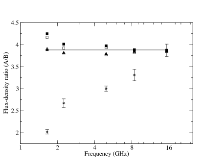
Figure 2: Observed (star symbols) and model-predicted image flux-density ratios versus frequency. The open and filled symbols correspond to the isothermal and non-isothermal fitting, respectively. The square symbols are used when image A is taken as the primary image and the triangle symbols are used when image B is taken as the primary image.

The results from the detailed analysis of the radio maps of the two images of B0218+357, A and B, and from applying the lens models are shown in Fig. 2. The line parallel to the $x$–axis is the image flux-density ratio of a background point-like source at the position of A1 (or B1) at 15.35 GHz, depicting the frequency-independent nature of the gravitational lensing effect. The model-predicted ratios for both isothermal and non-isothermal mass-radius profiles, obtained from using the observed brightness distributions of image A and image B separately, are shown as square or triangle symbols. Also shown as ‘stars’ are the image flux-density ratios calculated from the multi-frequency observations (M06), indicating clearly the frequency trend in the observed image flux ratios in B0218+357. As can be seen, for all four model-predictions the ratio remains the same to within $<4$ % except for 1.65 GHz using A as the primary image, where the ratio differs from a point-source model by about 8 % for the isothermal model and 10 % for the non-isothermal model. Furthermore, the change in the ratio due to the shift in the centroid position in image A at 1.65 GHz, as derived from the phase-reference observations in M06, is less than a percent.

Thus, our study of the effect of the interaction of frequency-dependent source structure with macro-model magnification gradient confirms that this cannot be the cause of the observed $\nu$–dependent image flux-density ratio in B0218+357. This analysis does show that the relative image-magnification estimated from applying the entire structure of image A at 1.65 GHz is significantly different from when the image-A centroid position at the same frequency is directly applied to the model. It is to be noted that the above 8 % to 10 % effect on the ratio is compatible with the values of relative image-magnification in the direction of the subcomponent newly-identified at 1.65 GHz only in image A, component 3. This is not surprising since the peak intensity of component 3 is comparable to that of components 1 & 2, and has a non-negligible effect on the centroid position in image A at this frequency. However, the change in the ratio is in a direction in which the relative image-magnification increases, opposite to the declining trend observed at decreasing frequencies. Finally, this study confirms that there can be departures from the general notion that the phenomenon of gravitational lensing preserves the spectrum of the background source in all the images. These departures can be seen as small deviations of the relative image-magnifications at any given frequency relative to the neighbouring frequencies in Fig. 2. This has been shown based on the frequency-dependent radio structure of the background source in B0218+357 and without invoking any other external mechanisms, some of which are described in Section 3.

3 Propagation effects

In this section the effects of free-free absorption and scattering on the properties of the B0218+357 images are investigated. Both these mechanisms require regions of plasma along the lines-of-sight to the image in consideration. The presence of a molecular cloud in front of image A provides an easy solution to this requirement as molecular clouds harbour sites of recent star formation, which through photoionization build up regions of ionized hydrogen around them.

3.1 Free-free absorption

We begin with the assumption that the radiation from image B after lensing by the spiral galaxy is unperturbed by any other physical process. To investigate whether image A suffers from free-free absorption, we envisage a giant Hii region, embedded in the molecular cloud presented above, directly in front of the image. Hii regions are formed around hot O– or early B–type stars that emit uv–photons capable of ionizing the hydrogen clouds out of which these stars form in the first place. The delicate balance between the heating and cooling mechanisms within such a photo-ionized plasma, which comprises mainly hydrogen atoms, results in an equilibrium electron temperature of $\sim 10^{4}$ K. We further assume that this Hii region covers the entire image structure at the lowest frequency, 1.65 GHz. This is the simplest scenario which can be considered in that it may well be modified to one consisting of several Hii regions residing within the same molecular cloud but at different spatial locations, which in projection cover the entire image. In the following we assume that the Hii region has a homogeneous distribution of electron density and a temperature in the range 4000 K to 10 000 K.

For Hii plasmas a state of Local Thermal Equilibrium (LTE) is a good assumption. This is because the thermal equilibrium is well maintained in such regions as any perturbation that enters into the system is quickly redistributed through Coulomb collisions amongst all the elements of the plasma. This validates the Kirchhoff law, so that the free-free absorption coefficient in the Rayleigh-Jeans regime is given by (see Rybicki & Lightman 1979; Brown 1987)

$$\alpha_{\mathrm{ff}}\;=\;3.19\,\times 10^{-7}\,\left(\frac{n_{\mathrm{e}}}{1\,\mathrm{cm}^{-3}}\right)^{2}\,\left(\frac{T_{\mathrm{e}}}{10^{4}\,\mathrm{K}}\right)^{-1.35}\,\left(\frac{\nu}{\mathrm{GHz}}\right)^{-2.1}\,\mathrm{pc}^{-1}\,$$ (5)

where $n_{\mathrm{e}}$ is the electron density, $T_{\mathrm{e}}$ is the electron temperature and $\nu$ is the observed frequency scaled by a factor of ($1+z_{\mathrm{l}}$), where $z_{\mathrm{l}}$ is the redshift of the lens galaxy. In deriving Eq. (5), a pure hydrogen cloud has been assumed and thus, $n_{\mathrm{e}}=n_{\mathrm{i}}$ and $Z=1$, where $n_{\mathrm{i}}$ is the ion density and $Z$ is the ionic charge. The intensity of background radiation that passes through an Hii region is modified according to the law of radiative transfer to

$$I_{\mathrm{ff}}(\nu,\tau)\;=\;I_{\mathrm{o}}(\nu)\,e^{-\tau_{\mathrm{ff}}(\nu)}\,,$$ (6)

where $I_{\mathrm{ff}}$ and $I_{\mathrm{o}}$ are the modified and background intensities, respectively, and $\tau_{\mathrm{ff}}$ is the optical depth equal to the integral of the free-free absorption coefficient over the path length through the plasma. Under the assumption of homogeneity in electron density and temperature, the optical depth is equal to $\alpha_{\mathrm{ff}}L$, where $L$ is the depth of the cloud. In the above, the source function, which under the condition of LTE is equal to the Planck blackbody spectrum, has been ignored since a source temperature of $\sim 10^{4}$ K is below the minimum brightness temperature that can be detected using VLBI. Introducing the physical parameter, Emission Measure ($EM=n^{2}_{\mathrm{e}}L$), the optical depth is

$$\tau_{\mathrm{ff}}\;=\;3.19\,\times 10^{-7}\,\left(\frac{T_{\mathrm{e}}}{10^{4}\,\mathrm{K}}\right)^{-1.35}\,\left(\frac{EM}{\mathrm{cm}^{-6}\,\mathrm{pc}}\right)\,\left(\frac{\nu}{\mathrm{GHz}}\right)^{-2.1}\,.$$ (7)

3.1.1 Parameter estimation of the Hii region

Table 2: The parameters derived for the Hii region in front of image A. $T$ is the temperature and $EM$ is the emission measure of the Hii region. Given also are the various combinations of the electron density and the depth of the cloud for given emission measures.

$T$	$EM$	$L$		$n_{\mathrm{e}}$
(K)	($\mathrm{cm}^{-6}$ pc)	(pc)	(mas)	($\mathrm{cm}^{-3}$)
$10^{4}$	($1.8\pm 0.3$) $\times$$10^{7}$	1	0.15	4243
		10	1.5	1342
		100	14	424
		200	28	300
4 000	($5.3\pm 0.9$) $\times$$10^{6}$	1	0.15	2302
		10	1.5	728
		100	14	230
		200	28	163

In order to determine the parameters of the Hii region, we assume the spectrum of image B to reflect the true source spectrum. Then, using the isothermal lens model described in Section 2.1 ($\beta=1$ in Table 1) and using the technique described in Section 2.2, the true spectrum of image A can be determined. Further, with the help of Eq. (7) and from the knowledge of the true and the modified spectrum of image A, Eq. (6) can be fitted to the observed flux-densities at different frequencies to determine the best fitting values of the plasma parameters. Unfortunately, the optical depth is degenerate to the following parameters which describe the Hii region: the electron density, the temperature and the depth of the cloud. But since the range of temperatures from observations of other Hii regions is known to be narrow, by fixing the temperature to two extreme values bracketing this range, the combination of the two remaining parameters, the emission measure, can be uniquely defined. The aim of this analysis is to find out whether the free-free absorption curve can be fitted at all to the observed spectrum of image A and also if the resulting values of $EM$ are physically meaningful.

The parameters of the hypothesized Hii region were estimated by, first, approximating the spectra of image B and the modelled image A by a synchrotron power-law,

$$F_{A}(\nu)\;\propto\;\nu^{-a}\;;\;F_{B}(\nu)\;\propto\;\nu^{-b}\;,$$ (8)

where $F_{A}(\nu)$ is the image A flux-density and $F_{B}(\nu)$ is the image B flux-density, and $a=0.153\pm 0.018$ and $b=0.147\pm 0.022$ are the power law indices fitted to their spectra. We note that the spectral indices for image A and image B assume slightly different values, in contradiction to the expectation of a constant magnification ratio for a point source from the model. This is due to the small differences in the modelled relative image-magnifications at varying frequencies, which in turn arise due to a frequency-dependent source structure (see Section 2.3). Substituting $F_{A}(\nu)$ for $I_{o}(\nu)$ in Eq. (6), the best-fitting value for $EM$ can be calculated using the $\chi^{2}$ minimization method to minimize the difference between the observed and the modelled image A flux-densities.

Figure 3: The free-free absorption curve (solid curve) fitted to the observed spectrum of image A (filled boxes). The modelled flux-densities of image A (open boxes) follow the measured flux-densities of image B (crosses) and their spectra (dotted lines) have nearly the same power law index.

Shown in Fig. 3 are the flux densities of image A (open boxes) modelled using the observed flux densities of image B (crosses). The fitted power-law spectra are shown in dotted lines. The free-free absorption curve (solid curve) is fitted to the observed flux-densities of image A (filled boxes). The various parameters, including the electron densities for different values of $L$, estimated for two values of temperatures are given in Table 2. The values of $EM$, although quite large, are consistent with those measured in giant Galactic Hii regions, and the estimations of $n_{\mathrm{e}}$ and $L$ are also in good agreement with those observed for Galactic and extragalactic Hii regions. In the present context the most meaningful combination of $n_{\mathrm{e}}$ and $L$ is the last entry in Table 2 for both $T$ values. This is because we have assumed that the Hii region covers all of image A, which at 1.65 GHz (the lowest frequency) has a deconvolved size of $\sim 28$ mas which translates into a physical size of about 200 pc at the redshift of the lens galaxy.

Given in Table 3 is a comparison between the image flux-density ratios obtained from the observations (second column) and those obtained after applying the free-free absorption model (third column), using Eq. (6). There is good agreement between these values and it is seen that the absorption can explain the observed trend very well at all the frequencies except at 4.96 GHz where the two values differ slightly, as is also visible from Fig. 3. As a further comparison, the ratios calculated from applying the SIEP model in Section 2.1, for the case where image-B is the primary image, are also given (the fourth column).

Table 3: Image flux-density ratios versus frequency as obtained from the observations (second column), the free-free absorption model (third column) and the isothermal lens-model (fourth column).

$\nu$ (GHz)	F${}_{\mathrm{A}}^{\mathrm{obs}}$/F${}_{\mathrm{B}}^{\mathrm{obs}}$	F${}_{\mathrm{A}}^{\mathrm{ff}}$/F${}_{\mathrm{B}}^{\mathrm{obs}}$	F${}_{\mathrm{A}}^{\mathrm{mod}}$/F${}_{\mathrm{B}}^{\mathrm{obs}}$
1.65	2.07$\pm 0.06$	1.99	3.90
2.25	2.71$\pm 0.11$	2.73	3.80
4.96	3.01$\pm 0.06$	3.46	3.76
8.40	3.41$\pm 0.15$	3.64	3.82
15.35	4.01$\pm 0.15$	4.01	3.84

For the above analysis even though, as already mentioned, we assumed a complete and uniform coverage, we tried to put constraints on the position and depth of the Hii region relative to the brightness distribution of image A at different frequencies. This turned out to be difficult due to an insufficient number of constraints available either from the observations used in this work (M06) or from the molecular (and atomic) line observations of this system by other authors. Even so, the maps of image A from these observations are strongly suggestive of a part of the absorption screen being directly in front of the centre-most region containing components 1 and 2. We arrived at this conclusion by mapping the inner subregions of image B (centered on B1), 2 mas by 1 mas in size, into equivalent regions in image A at all five frequencies. A comparison between the modelled spectrum of image A and the observed one showed that while there is a good match between the modelled and the observed flux-densities at 15.35 GHz, there is a clear indication of strong absorption at lower frequencies and that the fraction of the absorbed continuum increases with decreasing frequency.

From the above discussion, it can be concluded that the free-free absorption hypothesis is capable of reproducing the observed spectrum of image A and, thereby, of solving the image flux-density ratio anomaly in B0218+357. Furthermore, the values of the emission measure resulting from the fit for two extreme electron temperatures are quite reasonable in that similar values have been measured for Galactic and extragalactic Hii regions, lending further support to the hypothesis.

3.2 Scattering

Extragalactic sources are often found to be scatter-broadened by an intervening screen of turbulent plasma. The fluctuations in the plasma density induce variations in the refractive index, and in turn scatter the background radiation. This gives rise to two effects, scintillation and image- or scatter-broadening. There have been claims of scatter-broadening seen in gravitational lenses as well, such as PKS 1830-211 (Jones et al. 1996; Guirado et al. 1999), B1933+503 (Marlow et al. 1999), B0218+357 (Biggs et al. 2003), B0128+437 (Biggs et al. 2004) and PMN J1838-3427 (Winn et al. 2004).

Scattering by an infinite screen with homogeneous fluctuations in the electron density does not result in any changes in the flux-density of the background source. Based on symmetry arguments it can be proven that, in such a case, as much flux is scattered away as toward the line-of-sight to the observer, resulting in the conservation of flux-density. But this is no longer the case if there are variations in the statistical properties of the scattering screen. This includes the case where the scattering material appears in front of the scattered image only in parts, separated by ‘holes’ comprising neutral matter. In particular, if the scattering screen is truncated over the size of the scattered background image, it will lead to an attenuation of the source flux-density (Cordes & Lazio 2001). Thus, variations in the lensed image flux-densities because of an intervening scattering medium can occur only when there are discontinuities or variations in the scattering strength.

Scattering studies and measurements have been popular for over two decades now, and the basic physics behind the scattering mechanism is quite well-established (e.g. Rickett 1990; Narayan 1992; Goodman 1997). The regime of relevance in the present context is refractive scattering, as opposed to diffractive scattering. Refractive scattering is due to large-scale inhomogeneities in the medium with length scales, $r_{\mathrm{ref}}$, known as the refractive scale. This scale is much greater than what is known as the diffractive length-scale, $r_{\mathrm{diff}}$, which represents the transverse spatial-scale for which the root-mean-square phase change due to the intervening plasma blobs is equal to 1 rad. For refractive scattering, $\theta_{\mathrm{r}}=r_{\mathrm{ref}}/D_{\mathrm{l}}$ corresponds to the size of the scatter-broadened image of a point source projected back on the scattering screen (which is assumed to be in the lens plane), where $D_{\mathrm{l}}$ is the angular diameter distance from the observer to the scattering screen. For a source with a non-negligible size in comparison with the angular broadening size, the Gaussian-equivalent angular size of the image as measured is the quadrature sum of the intrinsic source-size and the refractive length scale. The latter scales as $\nu^{-2.2}$ [see Eq. (12)], which introduces the $\nu$–dependence of the scattering observables. Diffractive scattering, on the other hand requires sufficiently compact sources, $\theta<r_{\mathrm{diff}}/D_{\mathrm{l}}$, which for extragalactic scattering screens is rarely ever fulfilled, and therefore is not considered here.

Figure 4: Log-log plots of the geometric means of the axes of the elliptical Gaussians fitted to the smallest components in image A (right panel) and image B (left panel) versus frequency. Note that the scales on the $y$–axes are different for the two images.

To probe the relevance of scattering, the first issue that is addressed in the following is whether image A is affected by scattering at all. From an observational standpoint, the quantities which provide evidence for scattering are the image-sizes, in particular their dependencies on frequency, and temporal variations in the image flux-density. The latter can be ruled out since the image flux-density ratios measured for B0218+357 are independent of the time of observations, apart from the 5 % to 10 % level fluctuations arising due to the source variability and the time-delay between the images. To determine whether image A is scatter-broadened relative to image B (or vice-versa), we fitted two-dimensional elliptical Gaussians to the smallest detectable components in both the images at all frequencies. Shown in Fig. 4 are the equivalent circular radii, $R_{\mathrm{A}}$ and $R_{\mathrm{B}}$, of the ellipses fitted to these components plotted as a function of frequency. On fitting power-law curves through these data points $\sim\nu^{-k_{a,b}}$, where the power law indices, $k_{a}$ and $k_{b}$, correspond to the curves through A and B respectively, it is found that

$$k_{a}=1.40\pm 0.11\quad;\quad k_{b}=1.17\pm 0.05\,.$$ (9)

It should be pointed out that the scattered images produced by a homogeneous scattering screen, in general, have circular shapes due to isotropic scattering. Image A, on the contrary is elongated in roughly the same direction as predicted by the magnification matrix. In other words, the tangential eigen direction due to lensing is preserved. This is not an argument against scattering, however, because the phenomenon of gravitational lensing affects the scattering angle in the same way as the background source (see Appendix A), i.e. the scattering angle also gets magnified in the tangential direction.

The presence of two images of the same background source, if only one is assumed to be affected by scattering, can be used to advantage through determination of the true source size using the unaffected image. To determine the effects of scattering on the B0218+357 image properties, similar arguments are followed as those presented in Section 3.1 in that it is assumed that image B is unaffected by scattering or any other mechanism such as free-free absorption or milli-lensing (see Section 4). Then, the size of a component measured at any frequency in image B projected back to the source plane using a model will correspond to the intrinsic size of this component. From this, its equivalent size in image A can be calculated and compared to the observed size to yield a value for the refractive scale at that frequency. But this one-to-one correspondence can, from these observations, only be made at 15 GHz since at lower frequencies neither of the components 1 and 2 can be resolved, nor has any other distinct component been unambiguously detected in both the images. The third component in image A does not add any new information since it can either be that it is intrinsic to the source structure but due to insufficient resolution remains undetected in image B, or that it is produced by some other astrophysical mechanism. Thus, translating image B component-sizes to the true source sizes is not a reliable approach for analyzing the scattering hypothesis. Therefore, even though the similarity between the fitted power-law indices for both the images is highly suggestive of no, or hardly any, scattering in front of image A, the possibility cannot be ruled out completely. Accordingly, the scattering supposition in front of image A is pursued a little further in the hope to derive some meaningful limits.

Before deriving limits to $\theta_{\mathrm{r}}$, it should be recalled that the observed component-sizes are magnified by the lens galaxy. For a rough translation of a measured size in the image plane to its true size in the source plane, the following recipe is used. Consider a small elliptical background object with $a^{\prime}$ as the major axis and $b^{\prime}$ as the minor axis. Let the major axis be aligned with the direction of the tangential magnification. Then, for an isothermal mass profile, the source will be lensed into an elliptical image of size $\sqrt{(\mu a^{\prime})\times b^{\prime}}$, where $\mu$ is the tangential magnification (the radial magnification for an isothermal mass profile is unity). Equivalently, if an image-component has a size of $\sqrt{a\times b}$, its equivalent size in the source plane is $\sqrt{(a\times b)/\mu}$. For the current analysis, we use approximate values of 2 and 0.5 for the tangential magnification and de-magnification for images A and B, respectively. Consequently, the estimated sizes of the source-component 1, from the equivalent circular sizes of A1 and B1 at 15 GHz, are:

$$\theta_{\mathrm{s_{A}}}\,=\,0.25\pm 0.03\leavevmode\nobreak\ \mathrm{mas}\quad;\quad\theta_{\mathrm{s_{B}}}\,=\,0.28\pm 0.03\leavevmode\nobreak\ \mathrm{mas}\,.$$ (10)

Thus, there is a good agreement between the observations and the model-predictions at 15 GHz. But this is not surprising, since it is generally accepted that 15 GHz observations of this lens system are devoid of any discrepancies. The lens models discussed in Section 2.1 are derived assuming that the image flux-densities and positions observed at 15 GHz are free from any intervening astrophysical mechanisms since most interstellar effects go as $\nu^{-2}$.

Table 4: The scattering angular-sizes as a function of frequency for the Scattering Measure, $SM=2.12$ kpc $\mathrm{m}^{-20/3}$ (‘I’) and $SM=0.76$ kpc $\mathrm{m}^{-20/3}$ (‘II’), the quadrature difference of $\theta_{\mathrm{s_{A}}}$ and $\theta_{\mathrm{r(\mathrm{II})}}^{2}$, the component sizes in the image plane, $\theta_{\mathrm{A}}$ and $\theta_{\mathrm{B}}$, and the source plane, $\theta_{\mathrm{s_{A}}}$ and $\theta_{\mathrm{s_{B}}}$ [see Eq. (11) and Eq. (12)]

. $\nu$ (GHz) $\hat{\theta_{\mathrm{r}}}$ (mas) $\theta_{\mathrm{r}}$ (mas) $\theta_{\mathrm{A}}$ (mas) $\theta_{\mathrm{s_{A}}}$ (mas) $\sqrt{\theta_{\mathrm{r(\mathrm{II})}}^{2}-\theta_{\mathrm{s_{A}}}^{2}}$ $\theta_{\mathrm{B}}$ (mas) $\theta_{\mathrm{s_{B}}}$ (mas) I II I II 1.65 32.40 17.47 7.29 3.93 10.31$\pm$0.01 7.29 6.14 4.34$\pm$0.37 6.14 2.25 16.38 8.83 3.70 1.99 8.20$\pm$0.08 5.80 5.45 2.60$\pm$0.01 3.68 4.96 2.88 1.55 0.65 0.35 2.81$\pm$0.05 1.99 3.84 1.05$\pm$0.01 1.48 8.40 0.90 0.49 0.20 0.11 1.00$\pm$0.03 0.71 0.70 0.40$\pm$0.03 0.57 15.35 0.24 0.13 0.05 0.03 0.36$\pm$0.01 0.25 0.25 0.20$\pm$0.04 0.28

On the other hand, assuming that the component size of image A fitted at 1.65 GHz is solely due to scattering, an upper limit of $\theta_{\mathrm{r}}=\theta_{\mathrm{s_{A}}}=7.29$ mas is derived. It is to be noted that this is the observed scattering angle and depends upon the location of the scattering screen with respect to the source and the observer. The true scattering angle is

$$\hat{\theta_{\mathrm{r}}}\,=\,\frac{D_{\mathrm{s}}}{D_{\mathrm{ls}}}\,\theta_{\mathrm{r}}\,,$$ (11)

where $D_{\mathrm{ls}}$ is the angular diameter distance between the scattering screen (the lens galaxy) and the source. The quantity which is sought is the Scattering Measure ($SM$, in units of kpc $\mathrm{m}^{-20/3}$), which is the integral of the strength of the turbulence in the electron density distribution along the line-of-sight. Following the mathematical prescription given by Walker (1998, 2001) for a homogeneous scattering screen, the relation between the refractive scale for a point source ($\thinspace<\theta_{\mathrm{r}}$) and $SM$ is

$$SM\,=\,\left[1.6\times 10^{-2}\,\left(\frac{\hat{\theta_{\mathrm{r}}}}{\mathrm{mas}}\right)\,\left(\frac{\nu}{\mathrm{GHz}}\right)^{2.2}\,\right]^{5/3}\,\mathrm{kpc\leavevmode\nobreak\ m^{-20/3}}\,,$$ (12)

where $\nu$ is the radiation frequency at the redshift of the lens galaxy. Thus as pointed out earlier in this section, the scattering angle corresponding to the refractive scale, $\theta_{\mathrm{r}}$ [which is related to $\hat{\theta_{\mathrm{r}}}$ through Eq. (11)], scales as $\nu^{-2.2}$. Substituting $\hat{\theta_{\mathrm{r}}}$ and $\nu=1.65$ GHz in Eq. (12), a value of $SM=14.2$ kpc $\mathrm{m}^{-20/3}$ is obtained. It should be pointed out that the above limit on $\theta_{\mathrm{r}}$ is a secure upper limit since the intrinsic size of this component at 1.65 GHz is $>0$. In fact, $\theta_{\mathrm{s_{A}}}=7.29\pm 0.01$ mas is close to $\theta_{\mathrm{s_{B}}}=6.14\pm 0.52$ mas. Therefore, the true intrinsic source-size corresponding to the smallest component measured in image A at 1.65 GHz must be close to $\theta_{\mathrm{s_{A}}}$. This will decrease the scattering measure.

A second value of $SM$ can be estimated by assuming a true correspondence between the observed components at 1.65 GHz. Then, the quadratic difference in the back-projected sizes of the components can be attributed to the intervening scattering disk. In this case, $\theta_{\mathrm{r}}=\sqrt{\theta_{\mathrm{s_{A}}}^{2}-\theta_{\mathrm{s_{B}}}^{2}}=3.93$ mas. This leads to a value of $SM=5.1$ kpc $\mathrm{m}^{-20/3}$.

Substituting these values of scattering measure into Eq. (12), values of $\theta_{\mathrm{r}}$ can be determined at other frequencies as well and are given in Table 4. ‘I’ corresponds to when the A component at 1.65 GHz is used and ‘II’ corresponds to when the back-projected component in B at 1.65 GHz is assumed to represent the intrinsic source-size. Also given in Table 4 are the sizes of the image components in the image plane, $\theta_{\mathrm{A}}$ and $\theta_{\mathrm{B}}$, and projected back to the source plane, $\theta_{\mathrm{s_{A}}}$ and $\theta_{\mathrm{s_{B}}}$, and the quadrature difference of $\theta_{\mathrm{s_{A}}}$ and $\theta_{\mathrm{r(\mathrm{II})}}^{2}$. For the first method (‘I’), $\theta_{\mathrm{r}}$ and $\theta_{\mathrm{s_{A}}}$ can be directly compared and it is clearly seen that except at 1.65 GHz, there are strong inconsistencies at other frequencies. For the second method (‘II’), the difference between $\theta_{\mathrm{s_{A}}}$ and $\theta_{\mathrm{r(\mathrm{II})}}$, in quadrature, should be compared with $\theta_{\mathrm{s_{B}}}$. Once again, except at 1.65 GHz the values don’t match. It should be mentioned, nevertheless, that the two values for $SM$ derived in this section are comparable to the values of $SM$ calculated for other galactic and extragalactic scatter-broadened sources (Cordes & Lazio 2002; Spangler & Cordes 1998; Spangler et al. 1986).

Biggs et al. (2003) have suggested a much higher value of $SM=150$ kpc $\mathrm{m}^{-20/3}$ for B0218+357 which is atypical compared to those measured along typical lines of sight through the Galaxy but not inconsistent with the measurements in the direction of the Galactic center. However, their value is clearly not in agreement with the upper limit derived from these observations, given in Table 4. On the other hand, on account of free-free absorption, of which there is good evidence, it may well be that the estimated sizes in component A at lower frequencies are somewhat different from those due to scattering alone, which weakens any argument against the scattering hypothesis. In addition, it can also be that the scattering disk is such that it covers components 1 and 2 only, so that it has an observable effect on the size-measurements at 8.4 GHz. From comparing the back-projected sizes of components in A and B at 8.4 GHz, we find that a slightly bigger size of the image-A component requires a scattering measure of $\approx 48$ kpc $\mathrm{m}^{-20/3}$. In such a case, the effect of scatter-broadening would neither contradict the size-measurements at 15 GHz, on account of the $\theta_{\mathrm{r}}\sim\nu^{-2.2}$ frequency scaling, nor the low-frequency size-measurements, on account of a large intrinsic source-size. Such a scenario will be compatible with both, the claim made by Biggs et al. (2003) that image A is scatter-broadened at 8.4 GHz and also our measurements given in Table 4.

To summarize, it seems that scattering is not a satisfactory explanation for the flux ratio anomaly seen in B0218+357, even though it might contribute to scatter-broadening of the core-jet components in image A at higher frequencies. The reasons are two-fold. First, there is no strong evidence of $\nu$-dependent image-broadening for image A. This follows from the similarity of the $\nu$–dependencies of the component-sizes in both the images and under the assumption that image B does not suffer from any scattering. Moreover, the $\nu$–dependencies do not resemble the standard $\nu^{-2}$ scattering law. Instead, the index-values (slightly bigger than one) indicate that the increase in image-sizes with wavelength is intrinsic, common to most synchrotron self-absorbed sources. Second, even though the scattering measures derived in the above analysis are within the observed range of scattering measures in other systems, the back-projected component-size in image A and the size of the scattering disk are not compatible with each other at all five frequencies. However, these conclusions may be drawn only if the scattering strength is assumed to be homogeneous throughout the extent of the image A. If the scattering screen is clumpy and anisotropic, the analysis is no longer as straight-forward as that presented here.

4 Discussion

Two propagation effects, free-free absorption and scattering, have been investigated in the context of the flux ratio anomaly in the lens system B0218+357. Both these ISM effects have an inverse-frequency-squared dependence. In free-free absorption it is the optical depth that scales as $\nu^{-2.1}$, while in scattering it is the effective size of the scatter-broadened image that scales as $\nu^{-2.2}$. We assume that they occur in the interstellar-medium of the lens galaxy. In principle, these mechanisms can occur anywhere along the line-of-sight but the presence of a molecular cloud at the redshift of the lens galaxy lends the first possibility a higher probability. The image B properties, the flux-densities and sizes at varying frequencies, are assumed to remain unaffected by these processes.

To test the free-free absorption hypothesis, an Hii plasma in front of image A is envisaged which comprises free electrons that through Coulomb collisions absorb a part of the incoming image-A radiation, $I_{\mathrm{o}}$. The image A flux-density is attenuated by a factor, $e^{-\tau(\nu)}$, which depends upon the optical depth ($\tau$) of the cloud, and the spectrum of image A is altered. Using the isothermal lens-model described in Section 2.1, the observed flux-densities of image B are used to calculate the corresponding (unabsorbed) flux-densities of image A at all the frequencies. These values are used to fit the free-free absorption curve to the observed flux-densities of image A (Fig. 3) and the $EM$ of the Hii region is constrained to within $13$ % accuracy. This has been done for two values of the electron temperature, which is known to have a very narrow range from copious observational data of other Hii regions. The resulting values of $EM$ appear to be in the typical range observed in other galactic and extragalactic Hii regions. Thus, free-free absorption is an excellent candidate to explain the frequency-dependent image flux-density ratios.

From the lens models described in Section 2.1, image A lies at a projected distance of $2$ kpc from the lens centre. Its line-of-sight may well pass through one of the spiral arms of the galaxy, which are known to harbour extensive star forming regions and are rich in population I objects, such as young blue stars surrounded by Hii regions. In fact observations of other late-type spiral galaxies, such as M 51 (Lo et al. 1987), have shown that molecular gas, in the form of huge complexes of giant molecular clouds, is strongly confined to the spiral arms of a galaxy. Thus, it is possible that the image-A line-of-sight passes through such a region rich in gas and ionized plasmas (Hii regions). From the measurements of NH₃ absorption lines, Henkel et al. (2005) visualize the molecular absorber in front of image A to be elongated along a path with roughly constant galactocentric radius to reconcile with high source covering factors observed at mm-wavelengths. Elongated filament-like molecular clouds have been observed in the Milky Way, such as the Orion Giant Molecular Cloud (GMC) and the Monoceros GMC. For the free-free absorption hypothesis, it has been assumed that the Hii cloud covers image A completely at all the observed frequencies. At 1.65 GHz, the total extent of image A in the tangential direction is $\sim 28$ mas which corresponds to a linear size of $\sim 200$ pc in the lens plane. Such giant (and supergiant) Hii regions, although not ubiquitous, have indeed been observed, both as galactic and extragalactic. For example, the giant Hii region complex W49 in the Milky Way Galaxy has $L=150$ pc and $n_{\mathrm{e}}=100$ cm^-3, NGC 604 in M33 has $L=400$ pc and $n_{\mathrm{e}}\leq 60$ cm^-3 and NGC 5471 in M101 has $L=800$ pc and $n_{\mathrm{e}}=200$ cm^-3 (Shields 1990). Thus, the scenario in which the flux-density of image A is perturbed by a giant Hii region embedded in a turbulent molecular complex via free-free absorption can be easily envisioned. In reality, it may well be that there are several Hii regions embedded within the same molecular cloud but at different spatial locations and in projection cover the entire image A. Lastly, the question arises whether such a GMC in front of image A can, by virtue of its large mass, result in the magnification of image A, and possibly also a change in its position, differing from that predicted by the current lens-model. Solomon & Sanders (1980) estimated the mass-spectrum of the observed clouds in the Milky Way Galaxy and concluded that about 90 % of the mass of the molecular ISM is contained in GMCs with sizes larger than 20 pc and typical masses larger than $10^{5}\leavevmode\nobreak\ M_{\odot}$. On the other hand GMCs are not very centrally concentrated. Even though they might contain regions of high surface-density, such as compact vigorously star forming clumps, such scattered mass-condensations do not act as efficient lenses. Therefore we can ignore the gravitational effect of a plausible giant molecular complex on the properties of image A.

As a separate issue, we investigated whether there is any evidence of contribution from scattering in the lens galaxy to the disagreement between the predicted and the observed image flux-density ratios. The scattering hypothesis has been invoked for this lens system before by Biggs et al. (2003), who compared the 8.4 GHz maps of the images back-projected on the source plane and concluded that the subcomponents A1 and A2 have bigger sizes than B1 and B2. This, they claimed, was due to scatter-broadening in image A due to a turbulent medium in the lens galaxy, which is known to be ion and gas rich. In Section 3.2, similar comparisons between the image sizes have been tried with the present multi-frequency observations by applying a simple but effective method of determining the equivalent circular sizes of the components in the source plane from their fitted values in the image plane (the last two columns given in Table 4). But a direct comparison of the source-sizes derived from image A with those from image B presents a difficulty due to the ambiguity in the identification of the corresponding components in the images. Except at 15 GHz, due to different image magnifications it is not clear if the elliptical Gaussian fitted to an unresolved component in one image corresponds to the superposition of the same set of components in the source as fitted in the other image. The 8.4 GHz maps that Biggs et al. (2003) used for their analysis were obtained from global VLBI observations of B0218+357 with an rms noise of 30 $\mu$Jy $\mathrm{beam}^{-1}$. With this sensitivity, components 1 and 2 can easily be resolved in both the images. The rms noise in the 8.4 GHz maps of B0218+357 obtained from observations used in this work, in comparison, is at least a factor 10 higher and the components are unresolvable in image A and just resolvable in image B (this is because the component-separation along R.A. is larger in image B than in image A). The sizes of the components fitted to the images indicate, individually, a similar frequency-dependence, $\nu^{-k_{\mathrm{a,b}}}$, with $k_{\mathrm{b}}=1.2$ for image B, and a slightly stronger dependence with $k_{\mathrm{a}}=1.4$ for image A. It is to be noted that while the scattering angle scales with the inverse of frequency-squared, the intrinsic size has a much less pronounced dependence on the frequency. Based on extensive observational evidence it is seen that the angular size of a synchrotron self-absorbed source scales roughly as inverse frequency (Marscher 1977). Thus, the increase in the component-sizes in both the images can be an intrinsic effect. On the other hand, the scattering medium considered in this analysis is assumed to have statistically homogenous properties. It may well be that this assumption is not valid and that either the scattering measure has spatial variations transverse to the line-of-sight or the scattering screen is patchy with clumps of ionized material distributed over the image plane. Depending upon the distribution of ionized clumps, the image flux-density can either amplify or attenuate. In addition to this, effects from free-free absorption can further complicate the investigation of the scattering hypothesis by disturbing the flux-density distribution in image A, and thereby, altering the size-measurements derived from the elliptical Gaussian fits to the components. Therefore, even though there is no hard evidence for scattering found in our data, which dominates either the image sizes or the image flux-densities, we can not completely eliminate the possibility of a partially-covering scattering-screen.

One other plausible mechanism, which can lead the image magnifications to deviate from values dictated by simple macro-lensmodels, and which we have not addressed so far is milli-lensing or substructure due to the subhalos in the mass range from $10^{6}\leavevmode\nobreak\ M_{\odot}$ to $10^{9}\leavevmode\nobreak\ M_{\odot}$. Such subhalos are predicted by semi-analytic and numerical simulations of galaxy formation based on a CDM universe (e.g. Klypin et al. 1999; Moore et al. 1999). The number of such substructures are over-predicted by almost an order of magnitude compared to what is observed around the Milky Way Galaxy. The anomalous image flux ratios in galaxy scale lens systems are thought to be the first direct evidence of such small-scale power (e.g. Mao & Schneider 1998; Dalal & Kochanek 2002). But for two-image lens systems substructure effects cannot be examined with ease because of a severe shortage of constraints. In principle, a distribution of CDM-subclumps around one or both the images with a certain range of masses can reproduce any observations comprising image-positions and flux-ratios. But such a solution is not unique because in such a case the number of model parameters exceeds the number of constraints as obtained from observations. However, it is also predicted that the CDM mass-clumps around the lensed images produce astrometric shifts in the centroid of the image brightness-distribution (Dobler & Keeton 2005). These shifts depend on the source structure (thus frequency) and can be easily detected with high-resolution VLBI observations. The peak-to-peak image separation in B0218+357 does show an anomalous shifting at lower frequencies by about $\sim 2$ mas, therefore, entailing a need to follow-up the substructure hypothesis. For future studies, one way of analyzing the substructure hypothesis in B0218+357 further is by fixing the macro lens-model to the one obtained from the LensClean algorithm and generating random realizations of substructures (Dalal & Kochanek 2002) based on analytic approximations of substructure statistics.

Figure 5: Slices made through the core-components (1 & 2) and component 3 in image A at 1.65 GHz at a resolution of 7 mas and 2.25 GHz at a resolution of 5 mas.

The anomalous frequency-dependent peak-to-peak image separation might also find an explanation within the framework of free-free absorption. It may well be due to inhomogeneities in the absorbing-screen, which results in the centroid of the brightness distribution in image A moving toward the south-east direction, thereby, reproducing the separation trend. An inhomogeneous absorbing-screen may also provide an explanation for the occurrence of component 3 in image A at 1.65 GHz (as an alternative to the explanation offered in M06, namely that component 3 is a distinct real part of the background structure and does not appear in image B due to insufficient resolution). The VLBI maps of image A obtained from our data indicate a gradual appearance of the secondary maximum corresponding to component 3 with frequency. Even though it is visible most prominently at 1.65 GHz, there are hints that it exists even at 2.25 GHz. This is seen as an unresolved shoulder in the intensity cut at 2.25 GHz in image A, shown in Fig. 5, along the direction containing the core-jet subcomponents and component 3. It seems that the absolute intensity of this component at both frequencies is nearly the same but that the fractional intensity relative to the peak intensity (centered around the core-jet subcomponents) decreases from 1.65 GHz to 2.25 GHz. This might be due to a lower value of the absorption coefficient in the region of component 3 relative to the rest of the image area, which would have the effect of making the corresponding feature of the background source more prominent with decreasing frequencies.

5 Conclusions

We have shown that the image flux ratio anomaly in B0218+357 can be explained by invoking propagation effects, namely those arising due to free-free absorption, which is thought to occur in an ionized medium of the lens galaxy. It is believed that this is the first time that there has been offered a plausible explanation for the image flux ratio anomaly seen in B0218+357. This result has been achieved solely on the grounds of multi-frequency radio continuum observations presented in this work. The hypothesis receives support from radio and optical observations of molecular and atomic absorption lines which indicate the presence of an exotic interstellar medium in the lens galaxy, especially in front of image A.

A multi-frequency VLBI analysis of B0218+357 has led us to conclude that in order to investigate the causes of flux ratio anomalies evident in numerous lens systems, a multi-frequency approach is most yielding. Many lens systems are thought to be affected by dust-extinction in the optical (Falco et al. 1999), and by scintillation and scatter-broadening due to small-scale inhomogeneities in the ionized component of the ISM in the radio e.g. PMN J1838-3427 (Winn et al. 2004), B0128+437 (Biggs et al. 2004) and PKS 1830-211 (Guirado et al. 1999; Jones et al. 1996). The process of free-free absorption affects the spectra of the images causing them to be different from each other at low frequency, especially if the line-of-sight to an image passes through the galaxy centre or its spiral arms where the electron column densities are large, such as in PMN J1632-0033 (Winn et al. 2003) or, as has been shown in this work, JVAS B0218+357. Even milli-lensing, though gravitational in origin, can lead to $\nu$–dependent deviations in the properties of the lensed images. Previous CDM-substructure investigations have been made at a single frequency implying a frequency-independent effect of substructure on the image flux densities and image positions. However, the magnitude of the substructure effect on image magnifications changes with varying source size (especially apparent in the radio) and position relative to the Einstein radius of the perturber. Observations at several frequency bands at radio and optical wavelengths are essential to probe different processes, with different frequency-dependencies, acting on the image magnifications and to assess their contributions.

Further, we note that in order to use image flux-density ratios measured at radio wavelengths as constraints for lens modelling, the most trust-worthy values are those measured at high frequencies (such as 15 GHz and above) since the propagation effects at these frequencies are minimal. Also, any effects of substructure, such as different morphologies of jet images (Metcalf 2002), become more easily visible at such frequencies, which serve as further useful constraints for calculating substructure masses.

Appendix A Magnification of the scattering angle

In the presence of gravitational lensing, caused by an intervening massive object between the source and the observer, the scattering mechanism does not occur independently. We present a simple argument to show that the scattering angle is affected by lensing in the same way as the shape and size of the background source.

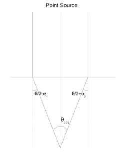
Figure 6: Scattering of a point source in the lens plane.

Consider a one-dimensional case of a point source which is scattered by the medium of an intervening galaxy. Let the scattering size be $\theta$. As the next step, we introduce the deflections contributed by gravitational lensing which results in ($\theta/2-\alpha_{1}$) and ($\theta/2+\alpha_{2}$) as the total deflection at the edges of the lensed image, where $\alpha_{1}$ and $\alpha_{2}$ are the angular deflections attributed to lensing. Then, the condition for the light rays from the lensed object to reach the observer is,

$$\theta_{\mathrm{obs}}\;=\;\theta+(\alpha_{2}-\alpha_{1})\;=\;\theta+\frac{\mathrm{d}\alpha}{\mathrm{d}\theta}\,\theta_{\mathrm{obs}}\;,$$ (13)

where $\theta_{\mathrm{obs}}$ is the observed angular extent of the lensed object. Hence

$$\theta_{\mathrm{obs}}\;=\;\mu\theta\,\quad;\quad\mu\;=\;\frac{1}{1-d\alpha/d\theta}\,,$$ (14)

where $\mu$ is the radial magnification produced by an axially symmetric lens (Schneider et al. 1992). Thus, the observed image size is the scattering size scaled by the lens-magnification factor. The result just derived does not apply only for radial magnification but is true in general.

References

- Biggs (2005) Biggs, A. 2005, in ASP Conf. Ser. 340: Future Directions in High Resolution Astronomy, ed. J. Romney & M. Reid, 433
- Biggs et al. (1999) Biggs, A. D., Browne, I. W. A., Helbig, P., et al. 1999, MNRAS, 304, 349
- Biggs et al. (2003) Biggs, A. D., Wucknitz, O., Porcas, R. W., et al. 2003, MNRAS, 338, 599
- Biggs et al. (2004) Biggs, A. D. et al. 2004, MNRAS, 350, 949
- Brown (1987) Brown, R. L. 1987, in Spectroscopy of Astrophysical Plasmas, 35–58
- Browne et al. (1993) Browne, I. W. A., Patnaik, A. R., Walsh, D., & Wilkinson, P. N. 1993, MNRAS, 263, 32
- Carilli et al. (2000) Carilli, C. L., Menten, K. M., Stocke, J. T., et al. 2000, Physical Review Letters, 85, 5511
- Carilli et al. (1993) Carilli, C. L., Rupen, M. P., & Yanny, B. 1993, ApJ, 412, L59
- Chengalur et al. (1999) Chengalur, J. N., de Bruyn, A. G., & Narasimha, D. 1999, in ASP Conf. Ser. 156: Highly Redshifted Radio Lines, ed. C. L. Carilli, S. J. E. Radford, K. M. Menten, & G. I. Langston, 228
- Cohen et al. (2000) Cohen, A. S., Hewitt, J. N., Moore, C. B., & Haarsma, D. B. 2000, ApJ, 545, 578
- Cohen et al. (2003) Cohen, J. G., Lawrence, C. R., & Blandford, R. D. 2003, ApJ, 583, 67
- Combes & Wiklind (1997) Combes, F. & Wiklind, T. 1997, ApJ, 486, L79
- Combes & Wiklind (1998) —. 1998, A&A, 334, L81
- Cordes & Lazio (2001) Cordes, J. M. & Lazio, T. J. W. 2001, ApJ, 549, 997
- Cordes & Lazio (2002) —. 2002, ArXiv Astrophysics e-prints
- Dalal & Kochanek (2002) Dalal, N. & Kochanek, C. S. 2002, ApJ, 572, 25
- Dobler & Keeton (2005) Dobler, G. & Keeton, C. R. 2005, MNRAS, 1122
- Falco et al. (1999) Falco, E. E., Impey, C. D., Kochanek, C. S., et al. 1999, ApJ, 523, 617
- Goodman (1997) Goodman, J. 1997, New Astronomy, 2, 449
- Guirado et al. (1999) Guirado, J. C. et al. 1999, A&A, 346, 392
- Henkel et al. (2005) Henkel, C., Jethava, N., Kraus, A., et al. 2005, A&A, 440, 893
- Jackson et al. (2000) Jackson, N., Xanthopoulos, E., & Browne, I. W. A. 2000, MNRAS, 311, 389
- Jones et al. (1996) Jones, D. L. et al. 1996, ApJ, 470, L23
- Kanekar & Briggs (2003) Kanekar, N. & Briggs, F. H. 2003, A&A, 412, L29
- Kanekar et al. (2003) Kanekar, N., Chengalur, J. N., de Bruyn, A. G., & Narasimha, D. 2003, MNRAS, 345, L7
- Klypin et al. (1999) Klypin, A., Kravtsov, A. V., Valenzuela, O., & Prada, F. 1999, ApJ, 522, 82
- Koopmans & de Bruyn (2000) Koopmans, L. V. E. & de Bruyn, A. G. 2000, A&A, 358, 793
- Lehár et al. (2000) Lehár, J., Falco, E. E., Kochanek, C. S., et al. 2000, ApJ, 536, 584
- Lo et al. (1987) Lo, K. Y., Ball, R., Masson, C. R., et al. 1987, ApJ, 317, L63
- Mao & Schneider (1998) Mao, S. & Schneider, P. 1998, MNRAS, 295, 587
- Marlow et al. (1999) Marlow, D. R. et al. 1999, MNRAS, 305, 15
- Marscher (1977) Marscher, A. P. 1977, ApJ, 216, 244
- Menten & Reid (1996) Menten, K. M. & Reid, M. J. 1996, ApJ, 465, L99
- Metcalf (2002) Metcalf, R. B. 2002, ApJ, 580, 696
- Mittal et al. (2006) Mittal, R., Porcas, R., Wucknitz, O., Biggs, A., & Browne, I. 2006, A&A, 447, 515
- Moore et al. (1999) Moore, B., Ghigna, S., Governato, F., et al. 1999, ApJ, 524, L19
- Muñoz et al. (2004) Muñoz, J. A., Falco, E. E., Kochanek, C. S., McLeod, B. A., & Mediavilla, E. 2004, ApJ, 605, 614
- Narasimha & Chitre (2004) Narasimha, D. & Chitre, S. M. 2004, Journal of Korean Astronomical Society, 37, 355
- Narayan (1992) Narayan, R. 1992, Phil. Trans. Roy. Soc., 341, 151
- O’Dea et al. (1992) O’Dea, C. P., Baum, S. A., Stanghellini, C., et al. 1992, AJ, 104, 1320
- Osterbrock (1974) Osterbrock, D. E. 1974, Astrophysics of gaseous nebulae (San Francisco: W. H. Freeman & Company)
- Patnaik et al. (1992) Patnaik, A. R., Browne, I. W. A., King, L. J., et al. 1992, LNP Vol. 406: Gravitational Lenses, 406, 140
- Rickett (1990) Rickett, B. J. 1990, ARA&A, 28, 561
- Rybicki & Lightman (1979) Rybicki, G. B. & Lightman, A. P. 1979, Radiative processes in astrophysics (New York, Wiley-Interscience, 1979. 393 p.)
- Schneider et al. (1992) Schneider, P., Ehlers, J., & Falco, E. E. 1992, Gravitational Lenses (Gravitational Lenses, XIV, 560 pp. 112 figs.. Springer-Verlag Berlin Heidelberg New York. Also Astronomy and Astrophysics Library)
- Shields (1990) Shields, G. A. 1990, ARA&A, 28, 525
- Solomon & Sanders (1980) Solomon, P. M. & Sanders, D. B. 1980, in Giant Molecular Clouds in the Galaxy, 41–73
- Spangler & Cordes (1998) Spangler, S. R. & Cordes, J. M. 1998, ApJ, 505, 766
- Spangler et al. (1986) Spangler, S. R., Mutel, R. L., Benson, J. M., & Cordes, J. M. 1986, ApJ, 301, 312
- Walker (1998) Walker, M. A. 1998, MNRAS, 294, 307
- Walker (2001) —. 2001, MNRAS, 321, 176
- Wiklind & Combes (1995) Wiklind, T. & Combes, F. 1995, A&A, 299, 382
- Winn et al. (2003) Winn, J. N., Rusin, D., & Kochanek, C. S. 2003, ApJ, 587, 80
- Winn et al. (2004) Winn, J. N. et al. 2004, AJ, 128, 2696
- Wucknitz et al. (2004) Wucknitz, O., Biggs, A. D., & Browne, I. W. A. 2004, MNRAS, 349, 14
- York et al. (2005) York, T., Jackson, N., Browne, I. W. A., Wucknitz, O., & Skelton, J. E. 2005, MNRAS, 357, 124