Formation and Collapse of Nonaxisymmetric Protostellar Cores in Planar Magnetic Interstellar Clouds: Formulation of the Problem and Linear Analysis

Abstract

We formulate the problem of the formation and collapse of nonaxisymmetric protostellar cores in weakly ionized, self-gravitating, magnetic molecular clouds. In our formulation, molecular clouds are approximated as isothermal, thin (but with finite thickness) sheets. We present the governing dynamical equations for the multifluid system of neutral gas and ions, including ambipolar diffusion, and also a self-consistent treatment of thermal pressure, gravitational, and magnetic (pressure and tension) forces. The dimensionless free parameters characterizing model clouds are discussed. The response of cloud models to linear perturbations is also examined, with particular emphasis on length and time scales for the growth of gravitational instability in magnetically subcritical and supercritical clouds. We investigate their dependence on a cloud’s initial mass-to-magnetic-flux ratio $\mu_{0}$ (normalized to the critical value for collapse), the dimensionless initial neutral-ion collision time $\tilde{\tau}_{\rm{ni,0}}$, and also the relative external pressure exerted on a model cloud $\tilde{P}_{\rm{ext}}$. Among our results, we find that nearly-critical model clouds have significantly larger characteristic instability lengthscales than do more distinctly sub- or supercritical models. Another result is that the effect of a greater external pressure is to reduce the critical lengthscale for instability. Numerical simulations showing the evolution of model clouds during the linear regime of evolution are also presented, and compared to the results of the dispersion analysis. They are found to be in agreement with the dispersion results, and confirm the dependence of the characteristic length and time scales on parameters such as $\mu_{0}$ and $\tilde{P}_{\rm{ext}}$.

1 Introduction

1.1 Background

In recent years there has been a steady and significant accumulation of observational data that support the idea that magnetic fields play a pivotal role in the evolution of interstellar molecular clouds and star formation. For instance, polarization maps of extended regions in clouds reveal large-scale magnetic fields that in several instances are aligned with the short axis of clouds (e.g. Pereyra & Magalhães 2004), which would be consistent with support from magnetic forces perpendicular to field lines. Infrared, far-infrared, and submillimeter maps of more localized regions show ordered field configurations with curvature, including “hourglass” shapes, that suggest dynamic interaction of magnetic fields and molecular cloud gas (Schleuning 1998; Schleuning et al. 2000; Fujiyoshi et al. 2001).

Interferometric polarization maps of molecular cloud cores by Lai et al. (2001, 2002) indicate similar ordered field structures. Furthermore, using a modification of the Chandrasekhar-Fermi (CF) method (Chandrasekhar & Fermi 1953), they estimated magnetic field strengths and energies that were large enough to exceed observed gas turbulence in their survey targets. A modified CF method was applied to the sub-mm polarization measurements of several prestellar cores by Crutcher et al. (2004), and they found that the mass-to-magnetic flux ratios of their cores were clustered about (within a factor $\sim 2$ above and below) the critical value for gravitational collapse. This result is consistent with earlier OH Zeeman determinations of the mass-to-flux ratios of protostellar cores (Crutcher 2004). Likewise, Curran et al. (2004) obtained sub-mm polarimetric images of two high-mass protostellar cores; a CF analysis of their data yielded mass-to-flux ratios for their two objects that were also nearly equal to the critical value for collapse. Finally, comparing CF results with OH Zeeman measurements for the immediate environment of the L184 prestellar core, Crutcher (2004) concludes that it may be an example of a nearly or barely critical core contained within a magnetically subcritical (i.e., supported) envelope. The grand picture painted by the various observational data above is one in which magnetic fields to a large degree control the structure and dynamics of star-forming molecular clouds, and has many elements of the original, unified theory of magnetically regulated star formation put forth early on by Mouschovias (1976, 1977, 1978, 1979; see, also, the review by Mouschovias & Ciolek 1999).

Ambipolar diffusion — the drift of neutral matter with respect to plasma and magnetic fields — initiates protostellar core formation in magnetically supported clouds. That is, because of imperfect collisional coupling between neutrals and charged particles (including dust grains; Ciolek & Mouschovias 1993, 1994), gravitationally-driven diffusion of matter in the inner flux tubes of clouds redistributes mass and magnetic flux that leads to the formation and subsequent dynamical collapse of supercritical cores or fragments within massive, subcritical envelopes. This process was exhibited in the two-dimensional axisymmetric magnetic cloud simulations of Fiedler & Mouschovias (1993), and the axisymmetric thin-disk model calculations by Ciolek & Mouschovias (1994, 1995) and Basu & Mouschovias (1994, 1995a,b). Uniformly, these studies demonstrated the formation of supercritical protostellar cores embedded in subcritical envelopes. They were also able to follow the resultant collapse of these cores well into the stage of dynamical infall, ending at the time when the central density was enhanced by a factor $\sim 10^{6}$.

Ciolek & Basu (2000; hereafter CB00) applied one of their axisymmetric magnetic disk models of core formation by ambipolar diffusion to the L1544 starless core. This model provided a good theoretical fit to the extended, subsonic infall profile as well as the distribution of mass in that core found by the earlier, complementary studies of Tafalla et al. (1998) and Williams et al. (1999). The predicted magnetic field strength in the CB00 model was later found to be in agreement with OH Zeeman observations of L1544 (Crutcher & Troland 2000; CB00). An analysis of submillimeter and millimeter maps and theoretical models of the dust temperature distribution in L1544 were found to be consistent with the emission distribution calculated from the CB00 model (Zucconi, Walmsley, & Galli 2001). Subsequent detailed, multispectral line maps used to further examine the kinematics within the L1544 core have also shown reasonable agreement between measured infall speeds and the CB00 predictions (Caselli et al. 2002). Finally, a multispectral survey by Crapsi et al. (2004) has found that some of the infall features of the prestellar core L1521F (which, like L1544, is in the Taurus complex) are comparable to those of the CB00 model.

However, despite the apparent successes of the aforementioned ambipolar diffusion models in describing the earliest stages of protostellar collapse, they are inherently limited because of their underlying assumption of axisymmetry. Axisymmetry is clearly a highly restrictive and idealized assumption, and is not likely to naturally occur in molecular clouds. In fact, sub-mm maps of star-forming clouds frequently indicate distinctively inhomogeneous and irregular large-scale structure and multiple cores (e.g., André, Motte, & Belloche 2001; Motte, André, & Neri 1998). Investigations at these wavelengths reveal irregularities on the scale of individual cores as well (e.g., Bacmann et al. 2000). Moreover, the observational studies of the L1544 core cited above find that it is definitely not axisymmetric. This is not a surprising result, as statistical analyses of data sets and catalogs of cores (e.g., Jones, Basu, & Dubinski 2001; Jones & Basu 2002; Kerton et al. 2003) reveal that their shapes can generally be best fit with a distribution of triaxial ellipsoids, which are typically more oblate than prolate.

Indebetouw & Zweibel (2000) simulated the formation of supercritical cores by ambipolar diffusion in infinitesimally thin, magnetic layers. Their models were two-dimensional and nonaxisymmetric, and they focused primarily on clouds that were initially subcritical. They followed the evolution of cores to when the maximum column density was a factor $\lesssim 5$ above the initial mean column density, and the irregular cores that developed were reminiscent of the sub-mm observations cited above. They also showed that the cores in their calculations developed on a timescale corresponding to the maximum linear growth rate of gravitational instability, and had a size equal to the corresponding wavelength (Zweibel 1998; see, also, § 3 below). Basu & Ciolek (2004; hereafter BC04) presented numerical models displaying the gravitational collapse of multiple dense, asymmetric protostellar cores in thin (yet, not infinitesimally so) planar magnetic clouds. One of their model clouds had an initial reference state with a mass-to-magnetic flux ratio that was exactly the critical value ($\mu_{0}=1$, see §§ 2.2 and 3.1 below). Another model of theirs was initially supercritical by a factor of 2 (i.e., $\mu_{0}=2$). They found that, in the initially critical model, transfer of mass by ambipolar diffusion resulted in the eventual formation of supercritical cores contained within subcritical envelopes, similar to that which occurred in their earlier axisymmetric models that started with initially subcritical conditions. By contrast, the initially supercritical model of BC04 had a much more rapid and dynamical infall, with significantly greater infall speeds (sonic and supersonic) extending over much larger regions. Based on the physically distinct and different predictions of these two models, they noted that molecular clouds that are supercritical by more than a factor $\sim 2$ would be incompatible with the generally observed subsonic infall motions.

1.2 Outline

In this paper, we present the formulation for modeling the formation and nonaxisymmetric collapse of protostellar cores in planar magnetic clouds. In § 2 we describe the fundamental assumptions and derive the necessary system of governing equations for a model cloud. The equations are put in nondimensional form, and the resulting free parameters of a model and their physical meaning are described. Our numerical method of solving the governing equations is also discussed. To provide a basis for understanding the underlying physics of ambipolar diffusion and gravitational collapse in magnetic sheets, the stability of model clouds is examined in § 3 by linearizing and Fourier-analyzing the governing equations. The results of the stability analysis are also compared with full numerical simulations of models in the limit of small-amplitude perturbations. In section § 4 we summarize our results, and discuss their relevance to forthcoming fully nonlinear studies of nonaxisymmetric core formation and collapse.

2 Physical Formulation

We model clouds as isothermal thin sheets with temperature $T$, embedded in a hot and tenuous external medium of constant pressure $P_{\rm{ext}}$. This simplifying assumption, the thin sheet approximation, is based on the numerical simulations of ambipolar-diffusion-initiated formation of cores by Fiedler & Mouschovias (1993), who found that two-dimensional, axially symmetric magnetically supported model molecular clouds rapidly flatten and establish force-balance along the direction of magnetic field lines, even while contraction and dynamical collapse took place in the direction perpendicular to the field. These results were soon afterward incorporated in the protostellar core formation studies of Ciolek & Mouschovias (1993; hereafter CM93) and Basu & Mouschovias (1994; hereafter BM94), who modeled molecular clouds as thin axisymmetric disks threaded by a vertical magnetic field, with hydrostatic equilibrium maintained along field lines at all times. Here we again adopt the formulation of CM93 and BM94, but now forego the restriction of axisymmetry.

The appealing feature of the thin-sheet approximation is that it can be used to model the physical processes necessary to core and star formation in a theoretically tractable and realistic way, including a self-consistent treatment of both magnetic pressure and tension forces. Another advantage of thin-sheet models is that because the physical equations have been simplified by integration in one dimension (here, in the direction of the vertical magnetic field), the problem has been substantially reduced from its full three-dimensional complexity. Because of this, sheet models can provide significantly higher spatial resolution, and require much less computational time and storage than fully three-dimensional cloud models. There is also some observational justification for the use of the thin sheet approximation. The often observed alignment, or at least close correlation, between the projected magnetic field direction from polarization measurements and the core minor axis is evidence for flattening along the field (Basu 2000). Furthermore, an analysis of core shapes by Jones et al. (2001) and Jones & Basu (2002) implies that they are preferentially flattened along one direction.

Of course, sheet models may not account for all of the observed morphological features of molecular clouds and their envelopes. Especially for those with large internal velocity dispersion, which can provide substantial support against self-gravity, and therefore be extended along magnetic field lines. It turns out though, that even in clouds or complexes with such substantial velocity dispersion or turbulence, thin-sheet models may still be used, so long as the application is restricted to dense sub-regions of the cloud. This has been demonstrated by Kudoh & Basu (2003, 2006), who analyzed the nonlinear support of stratified molecular clouds due to an ensemble of driven hydromagnetic waves. They found that because of density stratification, the largest, supersonic, velocities are in the low density envelope of a cloud, while a dense region near the midplane has transonic or subsonic motions. Hence, in this situation, thin-sheet models may reasonably be applied to a high-density fragment or sub-cloud, which will most likely be the site of subsequent star formation.

The most significant systematic source of possible inaccuracy of a thin-sheet model is that it typically overestimates the strength of the gravitational field in the equatorial plane (i.e., the plane of the disk) when compared to less condensed or concentrated systems. For instance, the critical wavelength for gravitational instability in very thin non-magnetic clouds is found to be half the value of the critical length found for an equilibrium layer with an exponential atmosphere. This can be seen by comparing our equation (40) derived in § 3.1, in the limit of zero external pressure, to equations (13-36) and (13-42) of Spitzer (1978). However, the equilibrium layer calculation assumes an infinite vertical extent, which reduces the system’s total gravitational binding energy; this is therefore an upper limit to the possible overestimate of calculating the gravitational field by using a thin disk. A better estimate was made by Kiguchi et al. (1987, see their Fig. 11), who showed that the magnitude of the planar gravitational field for an infinitesimally thin disk exceeds that of a flattened cloud of finite extent by at most only $\sim 40\%$, with the largest discrepancy between the two occurring for a very small region around the cloud center. BM94 presented a method of correcting for finite-thickness effects in the magnetic thin-disk approximation, deriving a quadratic correction (in terms of the local disk thickness) to the gravitational field. For the density regimes we intend to study ($\lesssim 10^{7}~{}{\rm{cm}^{-3}}$), the BM94 correction had the effect of altering the evolution of a model’s core by about 10% during the early stages of core evolution, to $\lesssim 30\%$ at much later stages. Finally, we note that because the planar magnetic field in the sheet is calculated the same way that the planar gravitational field is (see eqs. [15] - [16b] and [20] - [21b] below), there is also a comparable overestimate in the magnitude of the magnetic tension force. Since the magnetic tension force opposes the gravitational force, the overestimate in the value of the gravitational field due to the thin-sheet approximation is offset by a corresponding overestimate of the planar magnetic field, thereby reducing the net effect of overestimating both fields.

Thin-sheet models have been used by many workers in the field of molecular clouds and protostars. They were used early on by Narita, Hayashi, & Miyama (1984) to study star formation in axisymmetric, non-magnetic clouds. As mentioned above, the thin-sheet approximation was developed and applied to ambipolar diffusion and core formation in isothermal magnetic molecular clouds by CM93 (who included the effects of dust) and BM94 (who included rotation and magnetic braking). It was also later adopted by Li & Shu (1997a,b), who studied the equilibria and self-similar gravitational collapse of clouds with frozen-in magnetic flux (i.e., no diffusion). The approach to self-similar collapse during the later stage of core collapse with ambipolar diffusion in thin-disk clouds was described by Basu (1997). Ciolek & Königl (1998) incorporated the effect of the formation of a central gravitating point mass (a protostar) in numerical simulations of ambipolar-diffusion-driven dynamical core collapse in axisymmetric thin-disk clouds; a self-similar solution to this same problem was also provided by Contopoulos, Ciolek, & Königl (1998). Tassis & Mouschovias (2005a,b) also investigated this particular topic, further extending the analysis by including a detailed calculation of multi-fluid effects on the conductivity of the infalling gas during the later stages of supercritical core collapse and accretion.

A nonaxisymmetric ‘toy model’ idealization of a magnetically critical, flux-frozen turbulent sheet-like molecular cloud was suggested by Allen & Shu (2000). As noted in §1.1, Indebetouw & Zweibel (2000) first presented nonaxisymmetric simulations of core formation by ambipolar diffusion in infinitesimally thin magnetic sheets. BC04 presented models of nonaxisymmetric, gravitationally collapsing cores in magnetically critical and supercritical finite-thickness sheet-like molecular clouds, including ambipolar diffusion and its consequent effect on the dynamical evolution of clouds and cores. Li & Nakamura (2004) and Nakamura & Li (2005) used the thin-sheet approximation to examine the combined effect of turbulent initial conditions and ambipolar diffusion in forming supercritical cores.

2.1 Fundamental Equations

We present the necessary system of equations to model core formation in weakly ionized, magnetic interstellar clouds. As stated above, our model clouds are taken to be thin, with local vertical half-thickness $Z(x,y,t)$ in a Cartesian coordinate system. By a sheet being thin we mean that for any physical quantity $f(x,y,z,t)$, the criterion $f/|\nabla_{p}f|\gg Z$ is always satisfied, where $\nabla_{p}\equiv\mbox{\boldmath$\hat{x}$}\partial/\partial x+\mbox{\boldmath$\hat{y}$}\partial/\partial y$ is the planar gradient operator. The magnetic field threading a cloud is taken to have the form

$$\mbox{\boldmath$B$}(x,y,z,t) = B_{z,\rm{eq}}(x,y,t)\mbox{\boldmath$\hat{z}$}\hskip 160.00024pt{\rm for}~{}|z|\leq Z(x,y,t),~{}~{}~{}~{}$$ (1a)

$$\mbox{\boldmath$B$}(x,y,z,t) = B_{z}(x,y,z,t)\mbox{\boldmath$\hat{z}$}+B_{x}(x,y,z,t)\mbox{\boldmath$\hat{x}$}+B_{y}(x,y,z,t)\mbox{\boldmath$\hat{y}$}\hskip 15.50005pt{\rm for}~{}|z|>Z(x,y,t),~{}~{}$$ (1b)

where $B_{z,\rm{eq}}$ is the magnetic field strength in the equatorial plane of the cloud. In the limit $|z|\rightarrow\infty$, $\mbox{\boldmath$B$}\rightarrow B_{\rm ref}\mbox{\boldmath$\hat{z}$}$, where $B_{\rm ref}$ is a constant, uniform reference magnetic field very far away from the sheet. From now on, all physical quantities are understood to be a function of time $t$.

Note that the condition on the planar gradient of physical quantities within the thin-sheet approximation implies that $Z$ is the lower limit to the scales that can be described by our model. (For the gravitationally unstable modes, this condition is always satisfied, as the critical lengths always exceed this value — see eq. [40].)

The unit normal vector to the upper and lower surfaces of the sheet is

$$\mbox{\boldmath$\hat{n}$}(x,y,\pm Z)=\frac{\pm\mbox{\boldmath$\hat{z}$}\mp\left[(\partial Z/\partial x)\mbox{\boldmath$\hat{x}$}+(\partial Z/\partial y)\mbox{\boldmath$\hat{y}$}\right]}{\left[1+(\partial Z/\partial x)^{2}+(\partial Z/\partial y)^{2}\right]^{1/2}}~{}~{}.$$ (2)

Use of the integral form of Gauss’s law yields the continuity equation for the normal component of the magnetic field across the upper and lower surfaces of the sheet,

$$B_{z}(x,y,\pm Z)-B_{x}(x,y,\pm Z)\frac{\partial Z}{\partial x}-B_{y}(x,y,\pm Z)\frac{\partial Z}{\partial y}=B_{z,\rm{eq}}(x,y).$$ (3)

The system of multifluid equations necessary to model a weakly-ionized, magnetic, self-gravitating, isothermal molecular cloud is given by equations ($9a$)-($9m$) of CM93. (In this study we ignore the dynamical effect of interstellar dust grains. Hence, those terms representing grain contributions appearing in the system of fluid equations in CM93 are neglected.) As was done in CM93 and BM94, we simplify these basic equations in the thin-sheet approximation by vertically integrating them from $z=-Z(x,y)$ to $z=+Z(x,y)$. Doing so for the equation of mass continuity yields

$$\frac{\partial\sigma_{\rm n}}{\partial t}+\frac{\partial}{\partial x}(\sigma_{\rm n}v_{{\rm n},x})+\frac{\partial}{\partial y}(\sigma_{\rm n}v_{{\rm n},y})=0~{}~{},$$ (4)

where $\sigma_{\rm n}(x,y)\equiv\int_{-Z}^{+Z}\rho_{\rm n}(x,y)dz$ is the mass column density, and $v_{{\rm n},x}$ and $v_{{\rm n},y}$ are respectively the $x$- and $y$-components of the neutral velocity. In deriving equation (4) we have used the chain rule to obtain the velocity of the surface of the disk,

$$\frac{dZ}{dt}=v_{{\rm n},x}\frac{\partial Z}{\partial x}+v_{{\rm n},y}\frac{\partial Z}{\partial y}~{}~{}.$$ (5)

We have also employed a “one-zone” approximation, where we assume $z$-independence of physical quantities such as $\rho_{\rm n}$, and the planar velocity components $v_{{\rm n},x}$, and $v_{{\rm n},y}$. This approximation is also used for the planar components of the gravitational acceleration $g_{x}$ and $g_{y}$ that appear in the equations below.

To derive the $x$- and $y$-components of the force equation (per unit area) for the neutrals, we use equation (2) and the total (thermal plus Maxwell) stress tensor

$${\sf T}=-\left(\rho_{\rm n}C^{2}+\frac{B^{2}}{8\pi}\right){\sf 1}+\frac{\mbox{\boldmath$B$}\mbox{\boldmath$B$}}{4\pi}~{}~{},$$ (6)

where ${\sf 1}$ is the identity tensor, $C=(k_{\rm B}T/m_{\rm n})^{1/2}$ is the isothermal speed of sound; $k_{\rm B}$ is the Boltzmann constant, and $m_{\rm n}$ is the mean mass of a neutral particle (= 2.33 a.m.u. for an ${\rm H}_{2}$ gas with a 10% He abundance by number). Using equation (3), the symmetry conditions on $B_{z,\rm{eq}}$ and $B_{z}$ and the antisymmetry conditions on $B_{x}$ and $B_{y}$ about the equatorial plane, along with the divergence theorem, the integrated force equations are

$$\frac{\partial}{\partial t}\left(\sigma_{\rm n}v_{{\rm n},x}\right)+\frac{\partial}{\partial x}\left(\sigma_{\rm n}v_{{\rm n},x}^{2}\right)+\frac{\partial}{\partial y}\left(\sigma_{\rm n}v_{{\rm n},x}v_{{\rm n},y}\right) = \sigma_{\rm n}g_{x}-C_{\rm{eff}}^{2}\frac{\partial\sigma_{\rm n}}{\partial x}+F_{{\rm mag},x}~{}~{},$$ (7a)

$$\frac{\partial}{\partial t}\left(\sigma_{\rm n}v_{{\rm n},y}\right)+\frac{\partial}{\partial x}\left(\sigma_{\rm n}v_{{\rm n},y}v_{{\rm n},x}\right)+\frac{\partial}{\partial y}\left(\sigma_{\rm n}v_{{\rm n},y}^{2}\right) = \sigma_{\rm n}g_{y}-C_{\rm{eff}}^{2}\frac{\partial\sigma_{\rm n}}{\partial y}+F_{{\rm mag},y}~{}~{},$$ (7b)

where

$$F_{{\rm mag},x} = \frac{B_{z,\rm{eq}}}{2\pi}\left(B_{{}_{x,Z}}-Z\frac{\partial B_{z,\rm{eq}}}{\partial x}\right)$$ (8a)

$$+\frac{1}{4\pi}\frac{\partial Z}{\partial x}\left[B_{{}_{x,Z}}^{2}+B_{{}_{y,Z}}^{2}+2B_{z,\rm{eq}}\left(B_{{}_{x,Z}}\frac{\partial Z}{\partial x}+B_{{}_{y,Z}}\frac{\partial Z}{\partial y}\right)+\left(B_{{}_{x,Z}}\frac{\partial Z}{\partial x}+B_{{}_{y,Z}}\frac{\partial Z}{\partial y}\right)^{2}\right]~{},\hskip 20.00003pt$$

$$F_{{\rm mag},y} = \frac{B_{z,\rm{eq}}}{2\pi}\left(B_{{}_{y,Z}}-Z\frac{\partial B_{z,\rm{eq}}}{\partial y}\right)$$ (8b)

$$+\frac{1}{4\pi}\frac{\partial Z}{\partial y}\left[B_{{}_{x,Z}}^{2}+B_{{}_{y,Z}}^{2}+2B_{z,\rm{eq}}\left(B_{{}_{x,Z}}\frac{\partial Z}{\partial x}+B_{{}_{y,Z}}\frac{\partial Z}{\partial y}\right)+\left(B_{{}_{x,Z}}\frac{\partial Z}{\partial x}+B_{{}_{y,Z}}\frac{\partial Z}{\partial y}\right)^{2}\right]~{},$$

$B_{{}_{x,Z}}\equiv B_{x}(x,y,+Z)$, $B_{{}_{y,Z}}\equiv B_{y}(x,y,+Z)$, and

$$C_{\rm{eff}}^{2}\equiv\frac{\pi}{2}G\sigma_{\rm n}^{2}\frac{\left(3P_{\rm{ext}}+\frac{\pi}{2}G\sigma_{\rm n}^{2}\right)}{\left(P_{\rm{ext}}+\frac{\pi}{2}G\sigma_{\rm n}^{2}\right)^{2}}C^{2}$$ (9)

is the local effective sound speed. $G$ is the gravitational constant. The second term on the right hand sides of equations (8a) and (8b) represent small modifications to the magnetic force due to planar gradients of the half-thickness $Z$.

The equations for $v_{{\rm i},x}$ and $v_{{\rm i},y}$, the $x$- and $y$-components of the ion velocity, are similarly obtained by vertical integration of the force equation for the ions. They are, respectively,

$$v_{{\rm i},x} = v_{{\rm n},x}+\frac{\tau_{\rm{ni}}}{\sigma_{\rm n}}F_{{\rm mag},x}~{}~{},$$ (10a)

$$v_{{\rm i},y} = v_{{\rm n},y}+\frac{\tau_{\rm{ni}}}{\sigma_{\rm n}}F_{{\rm mag},y}~{}~{},$$ (10b)

where the neutral-ion collision (momentum-exchange) time

$$\tau_{\rm{ni}}=1.4\left(\frac{m_{\rm i}+m_{{}_{{\rm H}_{2}}}}{m_{\rm i}}\right)\frac{1}{n_{\rm i}\langle\sigma w\rangle_{\rm{i{\rm H}_{2}}}}~{}~{}.$$ (11)

The quantity $m_{\rm i}$ is the ion mass, which we take to be 25 a.m.u., the mass of the typical atomic ($\rm{Na}^{+}$, $\rm{Mg}^{+}$) and molecular ($\rm{HCO}^{+}$) ion species in clouds; $\langle\sigma w\rangle_{\rm{i{\rm H}_{2}}}$ is the neutral-ion collision rate, and is equal to $1.69\times 10^{-9}~{}{\rm{cm}}^{3}~{}{\rm s}^{-1}$ for ${\rm H}_{2}-{\rm{HCO}}^{+}$ collisions (McDaniel & Mason 1973). The factor of 1.4 in equation (11) accounts for the fact that the inertia of helium is neglected in calculating the slowing-down time of the neutrals by collisions with ions. (Further discussion on this point can be found in § 2.1 of Mouschovias & Ciolek 1999.) For the ion number density we assume a power-law behavior of the form

$$n_{\rm i}={\cal K}\left(\frac{n_{\rm n}}{10^{5}~{}{\rm{cm}^{-3}}}\right)^{k}~{}~{},$$ (12)

where ${\cal K}$ ($\simeq 3\times 10^{-3}~{}{\rm{cm}^{-3}}$) and $k$ ($\simeq 1/2$) are constants. In reality, the exponent $k$ is also a function of density (Ciolek & Mouschovias 1998), due to the fact that ambipolar diffusion can deplete the abundance of dust grains in a contracting core (Ciolek & Mouschovias 1996), which alters the rate of capture and recombination of ions and electrons on grain surfaces. However, we ignore this effect in our models for the time being.

Integrating the $z$-component of the force equation for the neutrals from $z=0$ to $z=+Z$, and requiring that there be hydrostatic equilibrium along field lines yields

$$\rho_{\rm n}C^{2}=\frac{\pi}{2}G\sigma_{\rm n}^{2}+P_{\rm{ext}}+\frac{\left(B_{{}_{x,Z}}^{2}+B_{{}_{y,Z}}^{2}+\left[B_{{}_{x,Z}}\frac{\partial Z}{\partial x}+B_{{}_{y,Z}}\frac{\partial Z}{\partial y}\right]^{2}\right)}{8\pi}~{},$$ (13)

where we have used the Gaussian relation for a thin sheet, $g_{z}(x,y,+Z)=-2\pi G\sigma_{\rm n}(x,y,+Z)$. As discussed in CM93 and BM94, the first two terms on the right side of equation (13) represent the self-gravitational stress and external pressure acting on a sheet, respectively. The latter term — not included in our earlier studies (e.g., see eq. [26] of CM93) — is the total magnetic “pinching” term due to magnetic pressure and tension stresses that act to compress the sheet. Although this last term is generally smaller than the others, we retain it nevertheless in our models, since it costs very little computationally to include it.

We use Poisson’s equation for a very thin sheet to solve for the gravitational potential $\psi$:

$$\nabla^{2}\psi(x,y,z)=4\pi G\sigma_{\rm n}(x,y)\delta(z).$$ (14)

Imposing the boundary condition $\lim_{|z|\rightarrow\infty}\psi(x,y,z)\rightarrow 0$, equation (14) can be solved by the method of Fourier transforms (e.g., Wyld 1976; Byron & Fuller 1992). Doing so, one finds for $z=0$,

$${\cal F}[\psi(x,y,0)]=-2\pi G\frac{{\cal F}[\sigma_{\rm n}(x,y)]}{k_{z}},$$ (15)

where ${{\cal F}}[f]$ is the two-dimensional Fourier transform of the function $f$, and $k_{z}=(k_{x}^{2}+k_{y}^{2})^{\text@frac{1}{2}}$ is a function of the planar wave numbers $k_{x}$ and $k_{y}$. Hence, at any time $t$ we can determine ${\cal F}[\psi]$ by calculating ${\cal F}[\sigma_{\rm n}]$. Inverting the transform then yields $\psi$ at that time, and from that we can calculate the gravitational field

$$g_{x}(x,y,0)=-\frac{\partial\psi(x,y,0)}{\partial x},$$ (16a)

$$g_{y}(x,y,0)=-\frac{\partial\psi(x,y,0)}{\partial y}.$$ (16b)

The magnetic field components $B_{{}_{x,Z}}$ and $B_{{}_{y,Z}}$ can be gotten in a similar fashion. Above the sheet, the magnetic field can be written in the form $\mbox{\boldmath$B$}(x,y,z>+Z)=\mbox{\boldmath$B$}^{\prime}(x,y,z)+B_{\rm ref}\mbox{\boldmath$\hat{z}$}$, where $\mbox{\boldmath$B$}^{\prime}$ is the reduced magnetic field. The assumption that the constant pressure external medium is hot and tenuous implies that it is also current-free ($\mbox{\boldmath$j$}_{\rm{ext}}=0$). Consequently, Ampere’s law gives $\nabla\times\mbox{\boldmath$B$}=0$ in the region above the sheet. Therefore, $\mbox{\boldmath$B$}^{\prime}=-\nabla\Psi$, where $\Psi$ is a scalar magnetic potential, that, because of Gauss’s law ($\nabla\cdot\mbox{\boldmath$B$}=0$), satisfies Laplace’s equation,

$$\nabla^{2}\Psi(x,y,z>+Z)=0.$$ (17)

From our earlier comments on the external field we have $\mbox{\boldmath$B$}^{\prime}\rightarrow 0$ very far from the sheet. Therefore,

$$\lim_{z\rightarrow\infty}\Psi(x,y,z)=0~{}~{}.$$ (18)

The boundary condition on $\Psi$ at $z=+Z$ is derived from the continuity equation (3) for the normal component of the magnetic field across the top surface of the sheet, which is, written in terms of $\Psi$,

$$\frac{\partial\Psi(x,y,+Z)}{\partial z}-\frac{\partial\Psi(x,y,+Z)}{\partial x}\frac{\partial Z}{\partial x}-\frac{\partial\Psi(x,y,+Z)}{\partial y}\frac{\partial Z}{\partial y}=-\left[B_{z,\rm{eq}}(x,y)-B_{\rm ref}\right]~{}~{}.$$ (19a)

In the thin-sheet approximation, this becomes

$$\lim_{+Z\rightarrow 0}\frac{\partial\Psi(x,y,+Z)}{\partial z}=-\left[B_{z,\rm{eq}}(x,y)-B_{\rm ref}\right]~{}~{}.$$ (19b)

The solution of the magnetic Laplace equation (17) for $\Psi$, subject to the boundary conditions (18) and (19b), can also be performed by Fourier transform, in analogy to what is done for the gravitational potential $\psi$. In the limit $+Z\rightarrow 0$, we find

$${\cal F}[\Psi(x,y,0)]=\frac{{\cal F}\left[B_{z,\rm{eq}}(x,y)-B_{\rm ref}\right]}{k_{z}}~{}~{}.$$ (20)

Once $\Psi$ is obtained, by inverting the transform, it follows that

$$B_{{}_{x,Z}} = \lim_{+Z\rightarrow 0}-\frac{\partial\Psi(x,y,+Z)}{\partial x},$$ (21a)

$$B_{{}_{y,Z}} = \lim_{+Z\rightarrow 0}-\frac{\partial\Psi(x,y,+Z)}{\partial y}~{}~{}.$$ (21b)

To close our system of equations, the evolution of the equatorial magnetic field in the plane of the sheet $B_{z,\rm{eq}}(x,y)$ is governed by the magnetic induction equation. For the density range we consider in our cloud models, $10^{3}~{}{\rm{cm}^{-3}}\lesssim n_{\rm n}\lesssim 10^{8}~{}{\rm{cm}^{-3}}$, the magnetic field is effectively “frozen” in the ion-electron plasma (see §§ 2.2 - 2.4 of Mouschovias & Ciolek 1999 for a discussion). Hence, advection of magnetic flux in our system is described by

$$\frac{\partial B_{z,\rm{eq}}}{\partial t}=-\frac{\partial}{\partial x}\left(B_{z,\rm{eq}}v_{{\rm i},x}\right)-\frac{\partial}{\partial y}\left(B_{z,\rm{eq}}v_{{\rm i},y}\right)~{}~{}.$$ (22)

2.2 Boundary Conditions, Uniform Background State and Initial Conditions

As described in the preceding section, model clouds are assumed to be isothermal thin planar sheets of infinite extent. We follow the evolution in a square Cartesian region of size $L$, with $-L/2\leq x\leq L/2$, $-L/2\leq y\leq L/2$. Periodic boundary conditions are used for all physical quantities.

Model clouds are initially characterized by a static, uniform background state with constant column density $\sigma_{\rm{n,0}}$ and equatorial magnetic field $B_{\rm ref}\mbox{\boldmath$\hat{z}$}$ (i.e., $B_{z,{\rm{eq}},0}=B_{\rm ref}$). From equations (7a), (7b), (16a), (16b), (21a), and (21b), it is seen that all forces — thermal, gravitational, and magnetic — are identically equal to zero in the background state. Evolution is initiated in a cloud by superposing a set of random column density perturbations, $\delta\sigma_{\rm n}(x,y)$ ($\ll\sigma_{\rm{n,0}}$, typically) on the uniform background state at time $t=0$. To maintain the same local mass-to-flux ratio $\sigma_{\rm n}/B_{z,\rm{eq}}$ in the initial state as in the reference state, the magnetic field is simultaneously perturbed, with $\delta B_{z,\rm{eq}}/B_{\rm ref}=\delta\sigma_{\rm n}/\sigma_{\rm{n,0}}$.

2.3 Dimensionless Equations and Free Parameters

The actual system of equations we solve are dimensionless versions of the equations presented in § 2.1 above. We adopt the following normalizations: the velocity unit is $[v]=C$, the column density unit is $[\sigma]=\sigma_{\rm{n,0}}$, unit of acceleration is $[a]=2\pi G\sigma_{\rm{n,0}}$, the time unit is $[t]=C/2\pi G\sigma_{\rm{n,0}}$, and the length unit is $[l]=C^{2}/2\pi G\sigma_{\rm{n,0}}$. From this system one can also construct a unit of magnetic field strength, $[B]=2\pi G^{1/2}\sigma_{\rm{n,0}}$. With these normalizations, the dimensionless equations that govern the evolution of a model cloud are

$$\frac{\partial\sigma_{\rm n}}{\partial t} = -\frac{\partial}{\partial x}(\sigma_{\rm n}v_{{\rm n},x})-\frac{\partial}{\partial y}(\sigma_{\rm n}v_{{\rm n},y})~{}~{},$$ (23a)

$$\frac{\partial}{\partial t}\left(\sigma_{\rm n}v_{{\rm n},x}\right) = -\frac{\partial}{\partial x}\left(\sigma_{\rm n}v_{{\rm n},x}^{2}\right)-\frac{\partial}{\partial y}\left(\sigma_{\rm n}v_{{\rm n},y}v_{{\rm n},x}\right)+\sigma_{\rm n}g_{x}-\tilde{C}_{\rm{eff}}^{2}\frac{\partial\sigma_{\rm n}}{\partial x}+F_{{\rm mag},x}~{}~{},$$ (23b)

$$\frac{\partial}{\partial t}\left(\sigma_{\rm n}v_{{\rm n},y}\right) = -\frac{\partial}{\partial x}\left(\sigma_{\rm n}v_{{\rm n},y}v_{{\rm n},x}\right)-\frac{\partial}{\partial y}\left(\sigma_{\rm n}v_{{\rm n},y}^{2}\right)+\sigma_{\rm n}g_{y}-\tilde{C}_{\rm{eff}}^{2}\frac{\partial\sigma_{\rm n}}{\partial y}+F_{{\rm mag},y}~{}~{},$$ (23c)

$$F_{{\rm mag},x} = B_{z,\rm{eq}}\left(B_{{}_{x,Z}}-Z\frac{\partial B_{z,\rm{eq}}}{\partial x}\right)$$ (23d)

$$+\frac{1}{2}\frac{\partial Z}{\partial x}\left[B_{{}_{x,Z}}^{2}+B_{{}_{y,Z}}^{2}+2B_{z,\rm{eq}}\left(B_{{}_{x,Z}}\frac{\partial Z}{\partial x}+B_{{}_{y,Z}}\frac{\partial Z}{\partial y}\right)+\left(B_{{}_{x,Z}}\frac{\partial Z}{\partial x}+B_{{}_{y,Z}}\frac{\partial Z}{\partial y}\right)^{2}\right],\hskip 25.00003pt$$

$$F_{{\rm mag},y} = B_{z,\rm{eq}}\left(B_{{}_{y,Z}}-Z\frac{\partial B_{z,\rm{eq}}}{\partial y}\right)$$ (23e)

$$+\frac{1}{2}\frac{\partial Z}{\partial y}\left[B_{{}_{x,Z}}^{2}+B_{{}_{y,Z}}^{2}+2B_{z,\rm{eq}}\left(B_{{}_{x,Z}}\frac{\partial Z}{\partial x}+B_{{}_{y,Z}}\frac{\partial Z}{\partial y}\right)+\left(B_{{}_{x,Z}}\frac{\partial Z}{\partial x}+B_{{}_{y,Z}}\frac{\partial Z}{\partial y}\right)^{2}\right],\hskip 25.00003pt$$

$$\tilde{C}_{\rm{eff}}^{2} = \sigma_{\rm n}^{2}\frac{\left(3\tilde{P}_{\rm{ext}}+\sigma_{\rm n}^{2}\right)}{\left(\tilde{P}_{\rm{ext}}+\sigma_{\rm n}^{2}\right)^{2}}~{}~{},$$ (23f)

$$\frac{\partial B_{z,\rm{eq}}}{\partial t} = -\frac{\partial}{\partial x}\left(B_{z,\rm{eq}}v_{{\rm i},x}\right)-\frac{\partial}{\partial y}\left(B_{z,\rm{eq}}v_{{\rm i},y}\right)~{}~{},$$ (23g)

$$v_{{\rm i},x} = v_{{\rm n},x}+\frac{\tilde{\tau}_{\rm{ni,0}}}{\sigma_{\rm n}}\left(\frac{\rho_{\rm n}}{\rho_{\rm{n,0}}}\right)^{k}F_{{\rm mag},x}~{}~{},$$ (23h)

$$v_{{\rm i},y} = v_{{\rm n},y}+\frac{\tilde{\tau}_{\rm{ni,0}}}{\sigma_{\rm n}}\left(\frac{\rho_{\rm n}}{\rho_{\rm{n,0}}}\right)^{k}F_{{\rm mag},y}~{}~{}$$ (23i)

$$\rho_{\rm n} = \frac{1}{4}\left(\sigma_{\rm n}^{2}+\tilde{P}_{\rm{ext}}+B_{{}_{x,Z}}^{2}+B_{{}_{y,Z}}^{2}+\left[B_{{}_{x,Z}}\frac{\partial Z}{\partial x}+B_{{}_{y,Z}}\frac{\partial Z}{\partial y}\right]^{2}\right)~{}~{},$$ (23j)

$$Z = \frac{\sigma_{\rm n}}{2\rho_{\rm n}}~{}~{},$$ (23k)

$${{\cal F}}[\psi] = -\frac{{\cal F}[\sigma_{\rm n}]}{k_{z}}~{}~{},$$ (23l)

$$g_{x} = -\frac{\partial\psi}{\partial x}~{}~{},$$ (23m)

$$g_{y} = -\frac{\partial\psi}{\partial y}~{}~{},$$ (23n)

$${{\cal F}}[\Psi] = \frac{{\cal F}[B_{z,\rm{eq}}-\tilde{B}_{\rm ref}]}{k_{z}}~{}~{},$$ (23o)

$$B_{{}_{x,Z}} = -\frac{\partial\Psi}{\partial x}~{}~{},$$ (23p)

$$B_{{}_{y,Z}} = -\frac{\partial\Psi}{\partial y}~{}~{},$$ (23q)

where $\rho_{\rm{n,0}}=(1+\tilde{P}_{\rm{ext}})/4$ is the dimensionless neutral mass density of the background state, and $\psi$ and $\Psi$ represent their values in the equatorial plane.

The above equations are, for the most part, the Cartesian analogs of the axisymmetric thin-disk equations presented in CM93 (their [66a]-[66q]) and BM94 (their [34a]-[34m]). A similar set of non-ideal MHD equations were used to model nonaxisymmetric core formation by Indebetouw & Zweibel (2000), with one particular exception: they modeled clouds as infinitesimally thin, with $Z=0$, and neglected the effect of magnetic pressure (i.e., the terms dependent on $Z$ in the equations above, and also in CM93 and BM94). This means that the stabilizing effect of magnetosound modes were not accounted for in the models of Indebetouw & Zweibel. Although this may be valid in some cases, there are, as we show below, some regions in the physically allowed parameter space for clouds in which magnetic pressure cannot be considered negligible compared to magnetic tension. The omission of magnetic pressure in these instances leads to inaccuracies in the length- and timescales for the onset of gravitational instability in magnetic clouds.

Equations (23a)-(23q) have several non-dimensional parameters. $\tilde{P}_{\rm{ext}}\equiv 2P_{\rm{ext}}/\pi G\sigma_{\rm{n,0}}^{2}$ is the ratio of the external pressure acting on the sheet to the vertical self-gravitational stress of the background state. The effect of ambipolar diffusion is expressed by the dimensionless initial neutral-ion collision time, $\tilde{\tau}_{\rm{ni,0}}\equiv 2\pi G\sigma_{\rm{n,0}}\tau_{\rm{ni,0}}/C$. The limit $\tilde{\tau}_{\rm{ni,0}}\rightarrow\infty$ corresponds to extremely poor neutral-ion collisional coupling, so that the ions and magnetic field have no effect on the neutrals. In the opposite limit, $\tilde{\tau}_{\rm{ni,0}}=0$, the neutrals are perfectly coupled to the ions, due to frequent collisions, and the magnetic field will be essentially frozen in the neutral matter. The parameter $k$ (=1/2, typically) is the exponent in the power-law expression (12) used to calculate the ion density as a function of the neutral density. As we noted earlier, this constant power-law assumption is only an approximation, since ambipolar diffusion has been shown to make $k$ a function of $n_{\rm n}$ in models with a more realistic ion chemistry network (Ciolek & Mouschovias 1998). Finally, $\tilde{B}_{\rm ref}=B_{\rm ref}/2\pi G^{1/2}\sigma_{\rm{n,0}}$ is the dimensionless magnetic field strength of the background state. For the units we have chosen for the column density and the magnetic field, the dimensionless mass-to-magnetic-flux ratio of the background state is

$$\mu_{0}\equiv 2\pi G^{{}^{\text@frac{1}{2}}}\frac{\sigma_{\rm{n,0}}}{B_{\rm ref}}=\frac{1}{\tilde{B}_{\rm ref}}~{}~{}.$$ (24)

This also happens to be the mass-to-flux ratio in units of the critical value for gravitational collapse, $1/2\pi G^{\text@frac{1}{2}}$ (Nakano & Nakamura 1978; see, also, § 3.1 below). Models with $\mu_{0}<1$ ($\tilde{B}_{\rm ref}>1$) are subcritical clouds, while those with $\mu_{0}>1$ ($\tilde{B}_{\rm ref}<1$) are supercritical.

Normally, we set $\sigma_{\rm{n,0}}$ by specifying the temperature $T$ and the density $n_{\rm{n,0}}$ of the background state. Using equation (13), and the fact that $C=0.188(T/10~{}{\rm K})^{1/2}~{}{\rm{km~{}s^{-1}}}$ for $m_{\rm n}=2.33$ a.m.u.,

$$\sigma_{\rm{n,0}}=\frac{3.63\times 10^{-3}}{(1+\tilde{P}_{\rm{ext}})^{\text@frac{1}{2}}}\left(\frac{n_{\rm{n,0}}}{10^{3}~{}{\rm{cm}^{-3}}}\right)^{\text@frac{1}{2}}\left(\frac{T}{10~{}{\rm K}}\right)^{\text@frac{1}{2}}~{}~{}{\rm g}~{}{\rm{cm}^{-2}}~{}~{}.$$ (25)

Both $C$ and $\sigma_{\rm{n,0}}$ are normalizing units that we have adopted for our cloud models. The units for length and time have the scalings

$$[l]=7.48\times 10^{-2}\left(\frac{T}{10{\rm K}}\right)^{\text@frac{1}{2}}\left(\frac{10^{3}~{}{\rm{cm}^{-3}}}{n_{\rm{n,0}}}\right)^{\text@frac{1}{2}}\left(1+\tilde{P}_{\rm{ext}}\right)^{\text@frac{1}{2}}~{}~{}{\rm{pc}},$$ (26)

and

$$[t]=3.98\times 10^{5}\left(\frac{10^{3}~{}{\rm{cm}^{-3}}}{n_{\rm{n,0}}}\right)^{\text@frac{1}{2}}\left(1+\tilde{P}_{\rm{ext}}\right)^{\text@frac{1}{2}}~{}~{}{\rm{yr}}.$$ (27)

The unit of mass is then

$$[M]=9.76\times 10^{-2}\left(\frac{T}{10~{}{\rm K}}\right)^{\mbox{$\frac{3}{2}$}}\left(\frac{10^{3}~{}{\rm{cm}^{-3}}}{n_{\rm{n,0}}}\right)^{\text@frac{1}{2}}\left(1+\tilde{P}_{\rm{ext}}\right)^{\text@frac{1}{2}}~{}M_{\odot}~{}.$$ (28)

It follows from equations (11), (12), and (25) that

$$\tilde{\tau}_{\rm{ni,0}}=\frac{0.241}{(1+\tilde{P}_{\rm{ext}})^{\text@frac{1}{2}}}\left(\frac{3\times 10^{-3}{\rm{cm}^{-3}}}{{\cal K}}\right)\left(\frac{10^{5}~{}{\rm{cm}^{-3}}}{n_{\rm{n,0}}}\right)^{k-\text@frac{1}{2}}~{}~{}.$$ (29)

From equations (24) and (25), a model’s reference magnetic field is given by

$$B_{\rm ref}=\frac{5.89\times 10^{-6}}{\mu_{0}(1+\tilde{P}_{\rm{ext}})^{\text@frac{1}{2}}}\left(\frac{n_{\rm{n,0}}}{10^{3}~{}{\rm{cm}^{-3}}}\right)^{\text@frac{1}{2}}\left(\frac{T}{10~{}{\rm K}}\right)^{\text@frac{1}{2}}~{}~{}{\rm G}.$$ (30)

2.4 Numerical Method of Solution

The system of dimensionless partial differential equations presented in the preceding section is solved by the method of lines (e.g., Schiesser 1991). This was used in the axisymmetric models of Morton, Mouschovias, & Ciolek (1994), Ciolek & Mouschovias (1994, 1995), and Basu & Mouschovias (1994, 1995a, b), and the nonaxisymmetric models presented in BC04. In this method, spatial derivatives within the PDEs are approximated by finite differences. The square computational domain of size $L\times L$ is discretized by dividing the region into $N^{2}$ uniform cells of size $L/N\times L/N$. $L$ is typically chosen to be a factor $\sim 4$ greater than the wavelength of maximum gravitational instability $\lambda_{\rm T,m}$ (see § 3.1 below). Three-point centered differences are used to approximate gradients. Advection of mass and magnetic flux is performed with the monotonic upwind scheme of van Leer (1979). The spatial discretization converts the system of PDEs to a system of coupled ordinary differential equations of the form $d{\mbox{\boldmath$y$}}/dt=\mbox{\boldmath$F$}(\mbox{\boldmath$y$},t)$, where $d\mbox{\boldmath$y$}/dt$, $y$, and $F$ are all vectors of dimension $VN^{2}$ ($V$ is the number of dependent variables). An implicit Adams-Bashforth-Moulton method is then used to time-integrate the resulting system of ODEs.

At each time step, numerical solution of the Fourier transform and also the inverse transform of quantities in the equations for the gravitational and magnetic potentials ([23l] and [23o]) is carried out with standard two-dimensional Fast Fourier Transform (FFT) techniques (e.g., Press et al. 1996).

3 Stability of Cloud Models

We now consider the response of model clouds to small-amplitude disturbances or perturbations. Such an analysis will illuminate the basic physics of gravitational instability in weakly ionized, sheet-like magnetic clouds, and will also provide the basis for understanding the length and time scales over which instabilities will develop in fully nonlinear calculations.

The linear stability of isothermal self-gravitating equilibrium layers with frozen-in magnetic fields was examined early on by Nakano & Nakamura (1978). They determined the critical mass-to-flux ratio for such objects, which is discussed further below. The gravitational stability of weakly-ionized and thin (but with finite thickness) axisymmetric magnetic disks was investigated by Morton (1991) and Morton & Mouschovias (1991, unpublished). Their analysis is very similar to the one that we present in this paper, and we reprise many of their results in the following section. A later, independent linear study of partially-ionized magnetic disks/sheets was also presented by Zweibel (1998). Similar to that which was done in Indebetouw & Zweibel (2000), Zweibel (1998) studied clouds that were infinitesimally thin ($Z=0$), and concentrated on those that are magnetically subcritical.

3.1 Linearization and Analysis

As is frequently done, the unperturbed zero-order (background) state of a model is assumed to be uniform and static. The dimensionless equations presented in § 2.3 above are linearized to first-order by writing, for any physical quantity,

$$f(x,y,t) = f_{0}+\delta f$$ (31)

$$= f_{0}+\delta f_{{}_{\rm a}}e^{i(k_{x}x+k_{y}y-\omega t)},$$

where $f_{0}$ refers to the unperturbed state, $\delta f$ is the perturbation and $\delta f_{{}_{\rm a}}$ is its amplitude, $k_{x}$ and $k_{y}$ are again the $x$ and $y$ wave numbers, and $\omega$ is the complex angular frequency. The perturbations are small, with $|\delta f_{{}_{\rm a}}|\ll f_{0}$. With regard to velocities, which have $\mbox{\boldmath$v$}_{0}=0$ because of the static assumption, it is understood that $|\delta\mbox{\boldmath$v$}|\ll$ characteristic signal speeds of the multifluid system (i.e., sound speed, Alfvén speed, etc.).

For the assumed type of perturbation (31), we can set $\partial/\partial t\rightarrow-i\omega$, $\partial/\partial x\rightarrow ik_{x}$, and $\partial/\partial y\rightarrow ik_{y}$. The dimensionless equations for a model cloud then become, collecting and retaining terms to first-order,

$$\omega~{}\delta\sigma_{\rm n} = k_{x}\delta v_{{\rm n},x}+k_{y}\delta v_{{\rm n},y}~{}~{},$$ (32a)

$$\omega~{}\delta v_{{\rm n},x} = \frac{k_{x}}{k_{z}}\left(\tilde{C}_{\rm{eff},0}^{2}k_{z}-1\right)\delta\sigma_{\rm n}+\tilde{B}_{\rm ref}\frac{k_{x}}{k_{z}}\left(1+k_{z}Z_{0}\right)\delta B_{z,\rm{eq}}~{}~{},$$ (32b)

$$\omega~{}\delta v_{{\rm n},y} = \frac{k_{y}}{k_{z}}\left(\tilde{C}_{\rm{eff},0}^{2}k_{z}-1\right)\delta\sigma_{\rm n}+\tilde{B}_{\rm ref}\frac{k_{y}}{k_{z}}\left(1+k_{z}Z_{0}\right)\delta B_{z,\rm{eq}}~{}~{},$$ (32c)

$$\omega~{}\delta B_{z,\rm{eq}} = \tilde{B}_{\rm ref}k_{x}\delta v_{{\rm n},x}+\tilde{B}_{\rm ref}k_{y}\delta v_{{\rm n},y}-i\tilde{\tau}_{\rm{ni,0}}\tilde{B}_{\rm ref}^{2}k_{z}\left(1+k_{z}Z_{0}\right)\delta B_{z,\rm{eq}}~{}~{}.$$ (32d)

From equation (23f), the reference state effective isothermal speed of sound is

$$\tilde{C}_{\rm{eff},0}=\frac{\left(1+3\tilde{P}_{\rm{ext}}\right)^{\text@frac{1}{2}}}{1+\tilde{P}_{\rm{ext}}}~{}.$$ (33)

In deriving the linearized system (32a)-(32d), we have used equations (23l)-(23n) to relate gravitational field perturbations to column density perturbations, (23o)-(23q) to relate planar magnetic field perturbations to those of the equatorial vertical magnetic field, and (23h) and (23i) to substitute the perturbed ion velocity components with those of the neutrals. The wavenumber $k_{z}$ has the same meaning as previously defined. A mode is unstable if the imaginary part of the complex frequency $\omega_{{}_{\rm I}}>0$. The growth timescale of the instability is $\tau_{\rm g}=1/\omega_{{}_{\rm I}}$.

The fundamental physics of the linear system is readily discerned from the various terms in equations (32a)-(32d): thermal-pressure and self-gravitational forces are proportional to perturbations in the column density in equations (32b) and (32c), and magnetic tension and pressure forces are proportional to perturbations in the equatorial magnetic field. The drift or diffusion of magnetic field and plasma with respect to the neutrals is represented by the term in the magnetic induction equation (32d) that contains $\tilde{\tau}_{\rm{ni,0}}$; comparison with the linearized mass continuity equation (32a) shows that, in the limit $\tilde{\tau}_{\rm{ni,0}}=0$, collisional coupling of the neutrals and ions (and therefore, the magnetic field) is instantaneous and perfect, and they all move together as a single fluid. In the opposite extreme, $\tilde{\tau}_{\rm{ni,0}}\gg 1$, neutral-ion collisions are infrequent, and the neutral and ion-magnetic field fluids are increasingly decoupled and move independently of one another.

The solution of the full dispersion relation for the gravitationally unstable mode of the linearized equations (32a) - (32d) are presented in Figure 1 for (a) $\tilde{\tau}_{\rm{ni,0}}=0$, (b) $\tilde{\tau}_{\rm{ni,0}}=0.04$, (c) $\tilde{\tau}_{\rm{ni,0}}=0.1$, (d) $\tilde{\tau}_{\rm{ni,0}}=0.2$, (e) $\tilde{\tau}_{\rm{ni,0}}=1$, and (f) $\tilde{\tau}_{\rm{ni,0}}=10$. The external pressure parameter for these models is $\tilde{P}_{\rm{ext}}=0.1$, which sets the dimensionless effective sound speed $\tilde{C}_{\rm{eff},0}=1.04$. (Note that $\tilde{C}_{\rm{eff},0}=1$ at $\tilde{P}_{\rm{ext}}=0$ and 1. $\tilde{C}_{\rm{eff},0}$ is maximal at $\tilde{P}_{\rm{ext}}=1/3$, and is equal to 1.061.) Displayed in each panel of Figure 1 is the growth time $\tau_{\rm g}$ as a function of the wavelength $\lambda$ ($=2\pi/k_{z}$), for various values of $\mu_{0}=1/\tilde{B}_{\rm ref}$. The separately labeled curves show the result for $\mu_{0}=0.5$, 0.8, 1, 1.1, 2, and 10, respectively. We are able to use $\lambda$ as the independent variable because the characteristic polynomial for our eigensystem is found to be only a function of $k_{z}=(k_{x}^{2}+k_{y}^{2})^{\text@frac{1}{2}}$. This means that to this order of approximation, all perturbations are independent of the planar angle of propagation $\theta$ [$=\tan^{-1}(k_{y}/k_{x})$].

Understanding the data presented in Figure $1a$ - $f$ is aided by examining the results for the instability growth timescale in the following two limits.

Limit 1: Flux-freezing, $\tilde{\tau}_{\rm{ni,0}}=0$.

In this limit, the neutrals, ions, and magnetic field respond as a single combined fluid, with the magnetic flux frozen in the neutrals, and the resulting dispersion relation is found to be

$$\omega^{2}-\left(\tilde{C}_{\rm{eff},0}^{2}+\tilde{B}_{\rm ref}^{2}Z_{0}\right)k_{z}^{2}-\left(\tilde{B}_{\rm ref}^{2}-1\right)k_{z}=0.$$ (34)

The gravitationally unstable mode corresponds to one of the roots of $\omega^{2}<0$, and occurs for $\tilde{B}_{\rm ref}<1$, or, equivalently, $\mu_{0}>1$. The growth timescale for this mode can be written as

$$\tau_{\rm g}=\frac{\lambda}{\left[2\pi(1-\tilde{B}_{\rm ref}^{2})(\lambda-\lambda_{\rm MS})\right]^{\text@frac{1}{2}}}~{}~{},$$ (35)

for $\lambda\geq\lambda_{\rm MS}$, where

$$\lambda_{\rm MS}\equiv 2\pi\left(\frac{\tilde{C}_{\rm{eff},0}^{2}+\tilde{B}_{\rm ref}^{2}Z_{0}}{1-\tilde{B}_{\rm ref}^{2}}\right)$$ (36)

is the critical or threshold wavelength for instability. The minimum growth timescale (= maximum growth rate) occurs at $\lambda_{\rm MS,m}\equiv 2\lambda_{\rm MS}$. The flux-freezing growth timescale (35) for our various model clouds is plotted as a function of $\lambda$ in Figure $1a$ - $f$, shown as open circles.

We have given to the critical wavelength $\lambda_{\rm MS}$ the subscript ‘MS’ because it is the maximum lengthscale that can be supported by both magnetic and thermal pressure effects, and therefore is related to magnetosound modes. This can be readily seen by noting that the dimensionless Alfvén speed in our model clouds is given by

$$\tilde{V}_{\rm{A,0}}=\frac{\tilde{B}_{\rm ref}}{\sqrt{2\rho_{\rm{n,0}}}}=\tilde{B}_{\rm ref}Z_{0}^{\text@frac{1}{2}},$$ (37)

(see eq. [23k]) and the fact that the dimensionless column density is unity for an unperturbed cloud. It follows then that the isothermal magnetosound speed (since we consider only isothermal perturbations in our models) in the adopted set of units is

$$\tilde{V}_{\rm{MS,0}} = \left(\tilde{C}_{\rm{eff},0}^{2}+\tilde{V}_{\rm{A,0}}^{2}\right)^{\text@frac{1}{2}}$$ (38)

$$= \left(\tilde{C}_{\rm{eff},0}^{2}+\tilde{B}_{\rm ref}^{2}Z_{0}\right)^{\text@frac{1}{2}}$$

$$= \tilde{C}_{\rm{eff},0}\left[1+\frac{2}{\mu_{0}^{2}}\frac{(1+\tilde{P}_{\rm{ext}})}{(1+3\tilde{P}_{\rm{ext}})}\right]^{\text@frac{1}{2}}~{}.$$

In the brackets of the last equality we have used eq. (33) and the relation

$$Z_{0}=\frac{2}{(1+\tilde{P}_{\rm{ext}})}~{}~{},$$ (39)

which follows from the linearization of equations (23j) and (23k), to eliminate $\tilde{C}_{\rm{eff},0}^{2}$ and $Z_{0}$ in terms of $\tilde{P}_{\rm{ext}}$. Examination of equation (36) reveals the presence of the magnetosound speed (38) in this expression, thus identifying the combined action of thermal and magnetic pressure in the support of a cloud against self-gravity. It also shows the importance of magnetic pressure in setting the instability timescale and the wavelength of maximum growth rate. For clouds that are close to being critical ($\mu_{0}\sim 1$), neglecting this effect (e.g., Zweibel 1998; Indebetouw & Zweibel 2000) can significantly underestimate $\tau_{\rm g}$ and $\lambda_{\rm MS,m}$.

When there is negligible magnetic support, that is, when $\tilde{B}_{\rm ref}\rightarrow 0$ ($\mu_{0}\rightarrow\infty$) it follows that $\tilde{V}_{\rm{MS,0}}\rightarrow\tilde{C}_{\rm{eff},0}$, and $\lambda_{\rm MS}\rightarrow\lambda_{\rm T}$, where

$$\lambda_{\rm T}\equiv 2\pi\tilde{C}_{\rm{eff},0}^{2}=\pi\left(\frac{1+3\tilde{P}_{\rm{ext}}}{1+\tilde{P}_{\rm{ext}}}\right)Z_{0}$$ (40)

is the critical thermal lengthscale. For this situation, the growth timescale for the unstable mode is still given by equation (35), with $\tilde{B}_{\rm ref}=0$, and $\lambda_{\rm T}$ replacing $\lambda_{\rm MS}$. The maximum growth rate for the unstable mode in this circumstance then occurs at $\lambda_{\rm T,m}\equiv 2\lambda_{\rm T}$.

Limit 2: Stationary magnetic field lines, $\omega\delta B_{z,\rm{eq}}=0$.

For this situation, which would be relevant to models with effective ambipolar diffusion, and therefore, relatively weak coupling of the neutrals to the ions and magnetic field, the resulting dispersion relation is

$$\omega^{2}+\frac{i}{\tilde{\tau}_{\rm{ni,0}}}\omega-\left(\tilde{C}_{\rm{eff},0}^{2}k_{z}^{2}-k_{z}\right)=0.$$ (41)

From this relation, one finds that an unstable mode exists for $\lambda>\lambda_{\rm T}$, and has a growth timescale

$$\tau_{\rm g}=\frac{2\tilde{\tau}_{\rm{ni,0}}\lambda}{\left[\lambda^{2}+8\pi\tilde{\tau}_{\rm{ni,0}}^{2}\left(\lambda-\lambda_{\rm T}\right)\right]^{\text@frac{1}{2}}-\lambda}~{}~{}.$$ (42)

The minimum growth time for this mode is at the wavelength $\lambda_{\rm T,m}$, defined above. The growth time (42) is also displayed as a function of wavelength in Figure $1a$ - $f$ (crosses).

As $\tilde{\tau}_{\rm{ni,0}}\rightarrow\infty$, $\tau_{\rm g}\rightarrow\lambda/\sqrt{2\pi(\lambda-\lambda_{\rm T})}$, which is identical to the result from equation (35) when $\tilde{B}_{\rm ref}=0$. This is because in both of these circumstances the magnetic field does not affect the neutrals: $\tilde{\tau}_{\rm{ni,0}}\rightarrow\infty$ corresponds to when there is no collisional coupling between the neutrals and ions (and, hence, the magnetic field). The ions are completely “invisible” to the neutrals in this situation, and there is no transmission of magnetic force to them via neutral-ion collisions. Similarly, when $\tilde{B}_{\rm ref}=0$, there is no magnetic field, and therefore magnetic forces do not contribute to the support or dynamics of a model cloud in that case.

With the results of the two limiting cases 1 and 2 described above in hand, the underlying physics of the gravitationally unstable modes presented in Figure $1a$ - $f$ is made more transparent. For instance, the models with the magnetic field frozen into the neutrals ($\tilde{\tau}_{\rm{ni,0}}=0$) displayed in Figure $1a$ are seen to be in exact agreement with the growth timescale predicted by equation (35). Particularly noteworthy is the dependence on the parameter $\mu_{0}$ ($=1/\tilde{B}_{\rm ref}$) for these models: there is no unstable, gravitationally collapsing mode for $\mu_{0}<1$. Moreover, models with $\mu_{0}\sim 1$ have minimum growth timescales at wavelengths $\lambda_{\rm MS,m}$ that are much larger than those for models with greater values of $\mu_{0}$. As an example, we note that $\lambda_{\rm MS,m}$ for the model with $\mu_{0}=1.1$ in Figure $1a$ is an order of magnitude greater than that in the model with $\mu_{0}=2$. The actual value of the growth timescale for the $\mu_{0}=1.1$ model is seen to be about an order of magnitude greater than that for the $\mu_{0}=2$ model as well. This is a consequence of there still being near-equality of gravitational and magnetic forces when $\mu_{0}$ is very close to unity.

When there is imperfect neutral-ion coupling ($\tilde{\tau}_{\rm{ni,0}}>0$), gravitational instability is possible even for model clouds with $\mu_{0}<1$. This can be seen in panels $b$ - $f$ of Figure 1. The timescale for the instability is typically greater than that for the supercritical flux-frozen models (Fig. $1a$), but it is finite. For these models, a Jeans-like growth of density perturbations occurs with the collapse moderated by the retarding collisional forces exerted on the neutrals as they diffuse through the plasma and field. A result of this type was first noted by Langer (1978). Models that are more subcritical are better approximated by the stationary field limit described above. This can be seen by the excellent agreement of the limiting growth timescale given by equation (42) — and also the wavelength of maximum growth ($\lambda_{\rm T,m}$) — with the dispersion curve for the $\mu_{0}=0.5$ model displayed in Figure $1b$ - $f$. As $\mu_{0}$ approaches unity, there is a transition of the growth timescale behavior from the stationary field/ambipolar diffusion limit (eq. [42]) and toward the flux-freezing limit (eq. [35]). For $\mu_{0}$ close to unity, the instability proceeds through a hybrid mode in which both ion-neutral drift and gravitational contraction with field-line dragging are active. As discussed above, the two limiting approximations approach one another for models with $\tilde{\tau}_{\rm{ni,0}}\gg 1$ and $\mu_{0}\gg 1$, since either limit describes clouds with effectively no magnetic support. This accounts for the near equality of all the model curves seen in Figure $1f$.

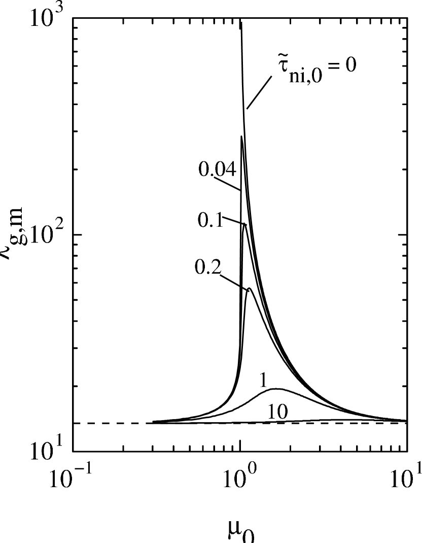
Figure 2: Wavelength with the minimum growth time (= maximum growth rate) as a function of initial mass-to-flux ratio. The displayed curves are for models with $\tilde{\tau}_{\rm{ni,0}}=0$, 0.04, 0.1, 0.2, 1, and 10, respectively. All models have $\tilde{P}_{\rm{ext}}=0.1$. The dashed curve is the value of $\lambda_{\rm T,m}$ for these models.

Figure 2 presents the wavelength $\lambda_{\rm g,m}$, which is defined as the wavelength $\lambda$ that has the minimum growth time, as a function of $\mu_{0}$ for models with the same values of $\tilde{\tau}_{\rm{ni,0}}$ and $\tilde{P}_{\rm{ext}}$ as in Figure $1a$ - $f$. For comparison, the dashed line in Figure 2 is the constant value of $\lambda_{\rm T,m}$ for those particular models. Consistent with our discussion above, we note that there is singular and limiting behavior of this lengthscale for the model cloud with $\tilde{\tau}_{\rm{ni,0}}=0$ and $\mu_{0}=1$. The value of $\lambda_{\rm g,m}$ is also seen to be especially sensitive to the value of $\mu_{0}$ for near-critical clouds with $\tilde{\tau}_{\rm{ni,0}}>0$, exhibiting a sharp, resonant-like peak in the region $\mu_{0}\sim 1$. Table 1 lists the ratio $\lambda_{\rm g,m}/\lambda_{\rm T,m}$ at the peak for each of the non-flux-frozen models in Figure 2. The peak ratio is largest for models with $\tilde{\tau}_{\rm{ni,0}}\lesssim 1$, while, for models with $\tilde{\tau}_{\rm{ni,0}}\gg 1$, magnetic field effects are barely transmitted to the neutrals (because neutral-ion collisions are very rare), and this ratio instead approaches unity.

Based on these results, we expect then, that clouds that are marginally or slightly supercritical will form cores that evolve more slowly, and have size scales (radii, and core spacing) significantly greater than that which will occur in clouds that are more highly supercritical. In addition, nearly critical clouds will also have size scales that are markedly larger than those in distinctly subcritical clouds. As we shall see in a following nonlinear study, this specific dependence of the gravitational instability on the initial mass-to-flux ratio leads to notable differences in the physical characteristics of collapsing cores in magnetic interstellar clouds that should be easily discerned by observations.

Figure $3a$ - $f$ shows the growth timescales for the same model clouds as in Figure 1, but with the dimensionless external pressure $\tilde{P}_{\rm{ext}}=10$. In the limit of large $\tilde{P}_{\rm{ext}}$, equation (23j) shows that the cloud is pressure confined, with $Z\propto\sigma_{\rm n}$ (eq. [23k]). As a result, a local peak in $\sigma_{\rm n}$ is a peak in $Z$. For this situation then, the top surface of the cloud looks like a dome and the external pressure force has horizontal components that point inward to the dome’s peak, acting in the same directions as the gravitational field components $g_{x}$ and $g_{y}$. This further enables the gravitational clumping, and decreases the growth timescale, appearing as a reduction of $\tilde{C}_{\rm{eff},0}$ in our equations. Because of this, the dimensionless sound speed $\tilde{C}_{\rm{eff},0}$ is decreased by a factor of 2.05 from its value in the models with $\tilde{P}_{\rm{ext}}=0.1$. This also reduces the growth timescale $\tau_{\rm g}$ and associated lengthscales $\lambda_{\rm MS}$ and $\lambda_{\rm T}$, since they are also functions of $\tilde{C}_{\rm{eff},0}$, and therefore, of $\tilde{P}_{\rm{ext}}$. The net effect is to shift and reduce the instability timescale and critical wavelengths by a corresponding factor from those seen in the models with lower external pressure. This means that clouds in regions with much greater external pressure (perhaps due to being embedded in a massive cloud complex or fragment, or adjoining hotter environments such as an HII region and/or shocked gas) will have characteristic sizes that are smaller when compared to clouds surrounded by lesser external pressures. However, the general behavior and physics of the models as a function of $\tilde{\tau}_{\rm{ni,0}}$ and $\mu_{0}$, including the applicability of the limiting analytical approximations discussed above, is similar to that seen in the previously described models with smaller $\tilde{P}_{\rm{ext}}$.

The wavelength with the minimum growth time $\lambda_{\rm g,m}$ is shown as a function of $\mu_{0}$ in Figure 4 for models with the same values of $\tilde{\tau}_{\rm{ni,0}}$ and $\tilde{P}_{\rm{ext}}$ as in Figure 3. It is again the case that, for clouds that are almost critical and with $\tilde{\tau}_{\rm{ni,0}}\lesssim 1$, the wavelength that has the most rapid gravitational response is significantly greater than in models that are farther away from $\mu_{0}=1$. The peak ratio values of $\lambda_{\rm g,m}$ to $\lambda_{\rm T,m}$ for the models with $\tilde{\tau}_{\rm{ni,0}}>0$ are also listed in Table 1. As before, this ratio is much greater for the models with $\tilde{\tau}_{\rm{ni,0}}\lesssim 1$.

3.2 Comparison to numerical simulations

We now compare the results of the dispersion analysis of the preceding section to simulations of the early evolution of model clouds governed by the full system of non-ideal magnetohydrodynamic equations (23a) - (23q). This system of equations is solved by a numerical code using the techniques described in § 2.4. The code was previously used to generate results for two model clouds whose nonlinear evolution was presented by BC04. During the early evolution of a model cloud, physical variables do not change very much from their initial state values. Hence, during this period the physical evolution should be close to that determined by the linear analysis above. Comparing the results of the early-time evolution of the full simulations to those of the dispersion analysis allows us to reinforce our understanding of the underlying physics governing the early evolution of a cloud — the precursor to the later nonlinear phase of evolution — as well as provide a useful benchmark and theoretical standard to establish the overall accuracy of our numerical code.

Because we are concerned with the linear stages of gravitational instability, we will confine our focus of the numerical simulations in this study to the evolution of the column density in model clouds. The detailed time-dependent behavior of other quantities, such as the velocity fields of the ions and neutrals, and the evolution and redistribution of mass in magnetic flux tubes will be described in a following paper.

3.2.1 Monochromatic perturbations

We follow the evolution of clouds initially given perturbations with a single wavelength $\lambda$. The evolution of a model cloud is initiated by imposing at time $t=0$ an initial (normalized) column density profile of the form

$$\sigma_{\rm n}(x,y,0)=1+\delta\sigma_{\rm n,a}\cos(2\pi x/\lambda),$$ (43)

that is, a uniform background state with a perturbation with amplitude $\delta\sigma_{\rm n,a}$. In using this particular perturbation, we make use of the fact that, as mentioned in § 3.1 above, the dispersion analysis indicates that the effects of linear disturbances are independent of the angle of propagation $\theta$. Since it really doesn’t matter for our purposes which direction of propagation we choose, we take $\theta=0$ (parallel to the $x$-axis), which means that $k_{y}=0$, and therefore $k_{x}=k_{z}=2\pi/\lambda$. The initial velocity and magnetic field are also perturbed in a way that is consistent with the system of equations (32a) - (32d) for the column density perturbation specified by equation (43). Solving for the initial perturbations $\delta v_{{\rm n},x}$, $\delta B_{z,\rm{eq}}$, and $\delta v_{{\rm n},y}$ in terms of the given $\delta\sigma_{\rm n}$, $k_{x}$, and $\tau_{\rm g}=i/\omega$ (which is a function of $\lambda$) from this set of equations yields

$$\delta v_{{\rm n},x}(x,y,0) = -\frac{\lambda}{2\pi\tau_{\rm g}}\delta\sigma_{\rm n,a}\sin(2\pi x/\lambda),$$ (44)

$$\delta B_{z,\rm{eq}}(x,y,0) = \frac{\lambda\tilde{B}_{\rm ref}}{\lambda+2\pi\tau_{\rm g}\tilde{\tau}_{\rm{ni,0}}\tilde{B}_{\rm ref}^{2}(1+2\pi Z_{0}/\lambda)}\delta\sigma_{\rm n,a}\cos(2\pi x/\lambda)~{},$$ (45)

and $\delta v_{{\rm n},y}(x,y,0)=0$. By specifying the relation between the perturbed physical variables in this way, we are basically selecting the eigenvector of the perturbation at the wavelength $\lambda$. Hence, the monochromatic perturbation excites a single eigenmode of a model cloud at $t=0$.

Not surprisingly, when we initiate the time evolution in this fashion, the subsequent evolution of a model cloud is simply the continued growth of the excited lone eigenmode. The left panel of Figure 5 displays the growth of the column density maxima for four different cloud models as a function of time. Each has $\tilde{\tau}_{\rm{ni,0}}=0.2$ and $\tilde{P}_{\rm{ext}}=0.1$. For all of these models, $\delta\sigma_{\rm n,a}=0.02$ and $\lambda=4\pi$. The calculations were performed on an equally spaced mesh of 32 $\times$ 32 cells on a square computational region of size $L=4\pi$ in each direction. Shown in that Figure (solid curves) is the evolution of the maximum reduced column density $\delta\sigma_{\rm n}(t)=\sigma_{\rm n}(t)-1$ for models with $\mu_{0}=0.5$, 1, 2, and 10. Also shown (dashed curves) is the growth of the column density perturbations that would occur as predicted by the linear relation for an unstable mode at the same location, $\delta\sigma_{\rm n}(t)=\delta\sigma_{\rm n,a}\exp(t/\tau_{\rm g})$. The values of $\tau_{\rm g}$ used to plot the curves are those derived from the earlier dispersion analysis for $\lambda=4\pi$, $\tilde{\tau}_{\rm{ni,0}}=0.2$ and $\tilde{P}_{\rm{ext}}=0.1$. From the data in Figure $1d$ we find that $\tau_{\rm g}=$ (20.3, 16.0, 4.34, 2.12) for $\mu_{0}=$ (0.5, 1.0, 2, 10). Comparing the numerical simulation results to the theoretical values predicted by the linear analysis indicates that they are in excellent agreement and overlap during much of the early evolution of each model. In fact, significant deviation ($\gtrsim 1\%$) between the simulation results and the linear predictions does not begin to occur until $\delta\sigma_{\rm n}$ has grown to $\sim 0.2$, which is well beyond what is generally considered the regime of linear growth. At later times nonlinear effects are evident, and the column density grows more rapidly and significantly exceeds that predicted by the linear analysis by the end of the period shown in Figure 5, when $\delta\sigma_{\rm n}=1$.

The growth of the column density perturbations in the numerical simulations at early times is entirely consistent with our discussion of the physical processes acting in the dispersion analysis in § 3.1. For instance, the linear analysis predicts that the onset of gravitational instability in the subcritical $\mu_{0}=0.5$ model is due to the action of ambipolar diffusion (see Fig. $1d$). Moreover, using the stationary field limit approximation (eq. [42]) to calculate $\tau_{\rm g}$ for this model ($\lambda_{\rm T}=6.75$ for these parameters) gives $\tau_{\rm g}=21.8$, which differs from the full dispersion analysis result quoted above by only $7\%$. The critical model $\mu_{0}=1$ and supercritical model $\mu_{0}=2$ are also heavily influenced by ambipolar diffusion, and they would not be able to collapse in its absence, because the excited wavelength for both of these models is in the region $\lambda_{\rm T}<\lambda<\lambda_{\rm MS}$. Thus, these two models lie in the transition region between diffusion-regulated and flux-frozen collapse for this particular wavelength, as noted in our discussion of these models in regard to Figure $1d$. Finally, the instability of the highly supercritical model $\mu_{0}=10$ occurs essentially with freezing of magnetic field lines in the neutral matter. For this model, $\lambda_{\rm MS}=6.93$ which is $<4\pi$. Using the flux-frozen approximate expression for the growth time given by equation (35) yields $\tau_{\rm g}=2.12$ for this model, which is exactly the same as the full dispersion relation solution, and is also in very good agreement with the model simulation’s early-time linear growth.

The right panel of Figure 5 shows the growth of the column density maxima in another four model clouds, with the same wavelength and parameters except $\tilde{P}_{\rm{ext}}=10$. The development of these higher-$\tilde{P}_{\rm{ext}}$ models is again seen to be in excellent agreement with the dispersion analysis for the linear stage of evolution. They are also in accordance with the values of $\tau_{\rm g}$ predicted by the analytic relations (42) and (35) for the subcritical and supercritical models, respectively.

We conclude then, that our numerical code accurately reproduces the physics of gravitational instability in planar magnetic model clouds.

3.2.2 White noise perturbations: the wavelength of minimum growth time $\lambda_{\rm g,m}$ and its dependence on $\mu_{0}$

In this subsection we consider cloud models that are given a spectrum of random, small-amplitude perturbations in the physical variables at $t=0$. The spectrum we use is white noise, i.e, flat, so that there is no preferred wavelength selected by the perturbations. However, we introduce damping so that wavelengths equal to twice the mesh spacing and smaller are negligible. The root-mean-square amplitude of the fluctuations in the initial state of a model cloud is 3% of the uniform background. The size of the computational region in each direction is $L=16\pi$, and the number of cells in each direction is $N=128$.

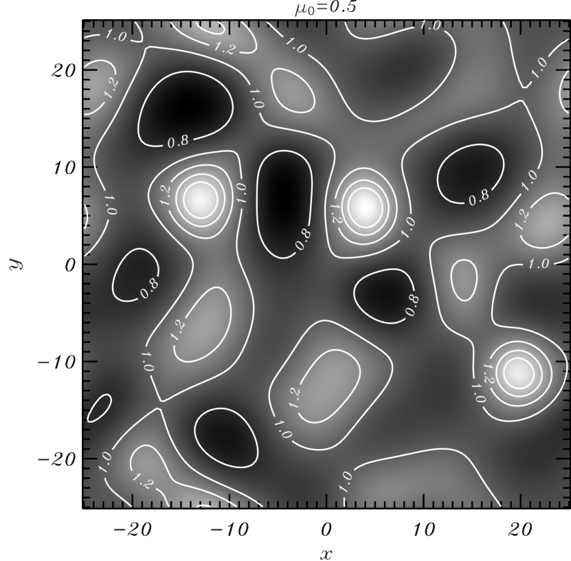
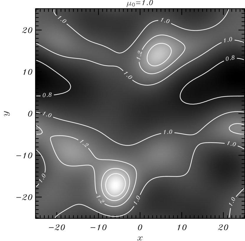
Figure 6: Column density contours of two model clouds that initially had random small-amplitude fluctuations in physical variables superposed on a uniform background state. The contours are overlaid on a grayscale image of the logarithm of the column density. At the time shown, the peak column density in each model is twice the value of the background state ($\sigma_{\rm n,max}=2$). Each model has $\tilde{\tau}_{\rm{ni,0}}=0.2$ and $\tilde{P}_{\rm{ext}}=0.1$. The left model has $\mu_{0}=0.5$, and the right one has the critical value $\mu_{0}=1$. The density contours range from 0.8 to 1.6, in steps of 0.2.

The white noise spectrum will excite an ensemble of eigenmodes with a wide range of wavelengths. The dominant evolutionary modes that will emerge from this ensemble of fluctuations and govern the subsequent evolution will be those grouped about the one with the minimum growth time. A cloud will then develop features with lengthscales comparable to the wavelength with the minimum growth time, $\lambda_{\rm g,m}$. That this intuitive notion is valid can be seen in Figure 6, which shows contour maps of the column density $\sigma_{\rm n}(x,y)$ in two model evolution simulations at the time for which the value of the maximum column density has grown to $\sigma_{\rm n,max}=2$ (twice the initial background value) in each model. Both models again have $\tilde{\tau}_{\rm{ni,0}}=0.2$ and $\tilde{P}_{\rm{ext}}=0.1$. The model displayed in the left panel is initially subcritical with $\mu_{0}=0.5$, and the one in the right panel started as a critical cloud with $\mu_{0}=1$. The density contours cover the range 0.8 to 1.6, in increments of 0.2. By the time that the contour snapshots are taken, nonlinear effects have set in. This is evidenced by column densities that are relatively large compared to that of the initial background state, and the beginning of nonaxisymmetric gravitational fragmentation (which will form protostellar cores) due to the interaction of various eigenmodes. Despite this, both cloud models retain a significant imprint from the predecessor linear stage of evolution: there is a nearly uniform separation between core fragments — defining here a core as the enclosed higher column density regions with $\sigma_{\rm n}>1.2$ — and the fragmentation scale for these nascent cores is close to $\lambda_{\rm g,m}$ in each model. For the model with $\mu_{0}=0.5$, Figure 2 indicates that $\lambda_{\rm g,m}=14$, while for the cloud with $\mu_{0}=1$, $\lambda_{\rm g,m}=24$. Examination of Figure 6 reveals that these scales correspond to the mean distance between the different $\sigma_{\rm n}=1.2$ contours for these models. Additionally, we note that the behavior of the fragmentation scale in these models as a function of $\mu_{0}$ is also consistent with the linear analysis. Notably, the average spacing between cores in the critical model evolution simulation is larger than that in the subcritical model, in line with the predicted dependence of $\lambda_{\rm g,m}$ on $\mu_{0}$ (see Fig. 2). This results in there being fewer cores within the same size region. In fact, according to Table 1 (see, also, Fig. $1d$), the maximal $\lambda_{\rm g,m}(=52.8)$ for these values of $\tilde{\tau}_{\rm{ni,0}}$ and $\tilde{P}_{\rm{ext}}$ occurs at $\mu_{0}=1.13$.

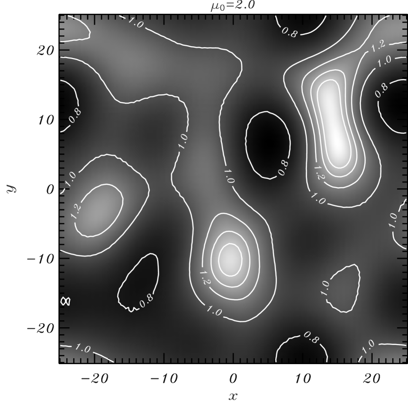
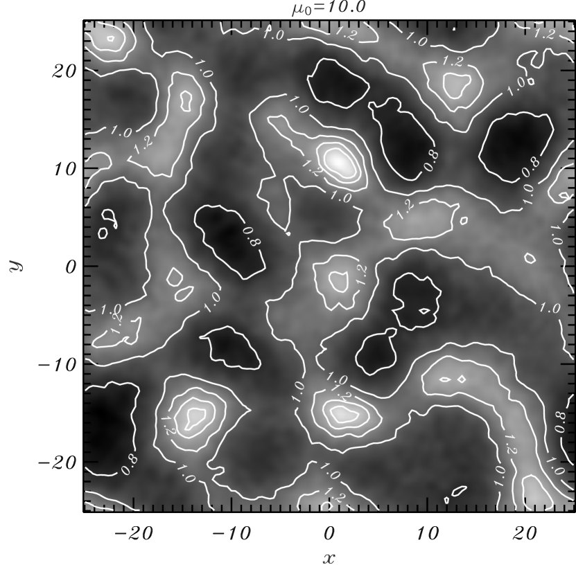
Figure 7: Same as in Fig. 6, but for supercritical models with $\mu_{0}=2$ (left) and $\mu_{0}=10$ (right).

Further confirmation that $\lambda_{\rm g,m}$ sets the characteristic lengthscales in clouds can be seen in Figure 7, which presents the column density plots of two more model clouds, with the same values of $\tilde{\tau}_{\rm{ni,0}}$ and $\tilde{P}_{\rm{ext}}$ as in Figure 6. The model in the left panel of Figure 7 is supercritical and has $\mu_{0}=2$. The linear analysis predicts $\lambda_{\rm g,m}=23$ for this model, which is indeed close to the the distance between core-bounding contours in that Figure. There are also relatively fewer cores that have formed, similar to that seen in the critical model. The similarity in the structural (lengthscale) properties of the $\mu_{0}=1$ and $\mu_{0}=2$ models is not surprising, as they have nearly equal values for $\lambda_{\rm g,m}$. However, the dynamical properties of the $\mu_{0}=1$ and $\mu_{0}=2$ models are quite different in the nonlinear regime, as shown by BC04. Specifically, the maximum velocities in the supercritical models become supersonic on scales that are well within the resolving power of modern observations. We defer the detailed discussion of the dynamical and related nonlinear evolution of cloud models to a study that will follow this paper, and to that already presented in BC04. Finally, the right panel of Figure 7 shows the column density contours for a highly supercritical model with $\mu_{0}=10$. For this model, $\lambda_{\rm g,m}=13$. This is also in agreement with the mean distance between cores in the contour plot. The lengthscales and number of cores in the highly supercritical model are akin to that seen in the subcritical $\mu_{0}=0.5$ model. This is no coincidence, since these two models have similar values of $\lambda_{\rm g,m}$. Although a somewhat counterintuitive result, this is because there is also a Jeans-like growth of density perturbations in the subcritical models, but it occurs on the much longer ambipolar diffusion timescale as neutrals drift past near-stationary plasma and magnetic field.

There are also some differences in the models in Figures 6 and 7 that become more pronounced with increasing initial mass-to-flux ratio: the cores become more nonaxisymmetric with greater values of $\mu_{0}$, showing enhanced elongation along a single axis. This second-order effect — an amplification of nonaxisymmetry due to the nonlinear interaction of certain eigenmodes for the more supercritical models — will be a topic of investigation in a following paper. And, as mentioned above, the dynamical properties of the model clouds, such as their velocity fields, are also markedly different, characteristically having greater infall velocities over larger scales with increasing $\mu_{0}$. This too will be studied further in a future paper. Despite these differences, we conclude from our representative evolution simulations that the gravitational fragmentation scale of a model cloud with an initial spectrum of perturbations is effectively the value of $\lambda_{\rm g,m}$ for that particular model. The fragmentation scale has a dependence on $\mu_{0}$ in agreement with the result of the linear analysis, especially with the prediction that near the critical value there is a dramatic increase in $\lambda_{\rm g,m}$. Because of this resonant-like behavior, clouds that are close to critical will have significantly larger size scales than in models that are more highly supercritical or more highly subcritical.

4 Summary

We have presented the formulation of physical models that we will use to study the nonaxisymmetric formation and self-gravitational collapse of protostellar cores in magnetic interstellar molecular clouds. Model clouds are partially ionized isothermal thin planar sheets with finite half-thickness $Z(x,y)$.

The system of equations that are used to govern the time evolution of model clouds contain four fundamental parameters, all defined in § 2.3. The first is the dimensionless background magnetic field strength of a cloud, $\tilde{B}_{\rm ref}$; the inverse of this parameter is the initial mass-to-magnetic flux ratio in units of the critical value for gravitational collapse, $\mu_{0}$. Clouds with $\tilde{B}_{\rm ref}>1$ ($\mu_{0}<1$) are subcritical and are initially magnetically supported, and cannot collapse in the absence of ambipolar diffusion. Models with $\tilde{B}_{\rm ref}<1$ ($\mu_{0}>1$) are supercritical from the outset and unable to support themselves against their own self-gravity. The next parameter is the normalized neutral-ion collisional momentum-exchange time $\tilde{\tau}_{\rm{ni,0}}$. It is a measure of the efficiency of ambipolar diffusion in model clouds: $\tilde{\tau}_{\rm{ni,0}}\rightarrow 0$ corresponds to very effective momentum transfer and collisional coupling of neutrals and ions, resulting in freezing of magnetic flux in the neutral matter. In the opposite limit of $\tilde{\tau}_{\rm{ni,0}}\gg 1$, collisions are so infrequent that the neutrals are essentially decoupled from the plasma and magnetic field, and magnetic forces contribute negligibly to the support and evolution of a model cloud. $\tilde{P}_{\rm{ext}}$ is the ratio of the external pressure to the vertical self-gravitational stress in the initial uniform reference state of a model cloud. The final parameter is the exponent $k$ in the power-law expression used to calculate the ion density as a function of the neutral density.

We also investigated the linear stability of model clouds, and how the growth times $\tau_{\rm g}$ and critical wavelengths of the gravitationally unstable modes depend on $\mu_{0}$, $\tilde{\tau}_{\rm{ni,0}}$, and $\tilde{P}_{\rm{ext}}$. Analytic expressions for $\tau_{\rm g}$ and the critical wavelengths were derived for the limits of weak and strong ambipolar diffusion. These expressions (eqs. [35] and [42]) agreed well with the full dispersion results in these limits.

Models with frozen-in magnetic flux ($\tilde{\tau}_{\rm{ni,0}}=0$) are gravitationally unstable when they are supercritical and the wavelength of a perturbation exceeds the magnetosound critical wavelength $\lambda_{\rm MS}$. For finite thickness clouds, magnetic pressure contributes substantially to setting the value of $\lambda_{\rm MS}$ and $\tau_{\rm g}$ when $\mu_{0}\sim 1$. Ambipolar diffusion ($\tilde{\tau}_{\rm{ni,0}}>0$) allows clouds to be unstable even when subcritical, so long as the perturbation’s wavelength is greater than the thermal critical wavelength $\lambda_{\rm T}$ ($\lambda_{\rm T}\leq\lambda_{\rm MS}$, see eqs. [36] and [40]). The instability modes of clouds with $\tilde{P}_{\rm{ext}}>1$ behave qualitatively the same way as for those with $\tilde{P}_{\rm{ext}}\leq 1$, except that quantitatively their critical wavelengths and growth times are reduced, due to the effective retarding sound speed being decreased at higher external pressures. The dispersion analysis also revealed how the wavelength with the minimum growth time, $\lambda_{\rm g,m}$, behaves as a function of $\mu_{0}$. For models with $\tilde{\tau}_{\rm{ni,0}}>0$, $\lambda_{\rm g,m}$ has a resonance at a value of $\mu_{0}$ that is usually just slightly greater than the critical value $\mu_{0}=1$. Because of this resonance, a model cloud with $\mu_{0}\sim 1$ will have a $\lambda_{\rm g,m}$ that is significantly greater when compared to that of models that are much more sub- or supercritical.

In addition to providing basic insight to the physics of gravitational instability in partially ionized media, the linear analysis was also used as a theoretical standard to test the accuracy of our numerical method of solution of the full set of nonlinear equations (eqs. [23a] - [23q]) that govern the time evolution of a model cloud. The early-time evolution of several cloud simulations given an initial monochromatic perturbation of wavelength $\lambda$ was compared to the predicted value of the growth timescale from the dispersion analysis. The temporal growth of the column density maxima in each model simulation was in excellent agreement with the theoretically predicted values of $\tau_{\rm g}$, thus establishing the accuracy of our non-ideal magnetohydrodynamic computational code.

Finally, we presented a suite of model simulations that had their evolution initiated by fluctuations with a spectrum of wavelengths, following their evolution a little beyond the linear growth phase. The characteristic fragmentation scale that developed in these models tends to correspond to the wavelength with the minimum growth time $\lambda_{\rm g,m}$ of the initial state. The resonance behavior of $\lambda_{\rm g,m}$ for clouds with the parameter $\mu_{0}$ near the critical value — as predicted by the linear analysis — was also in evidence in the numerical simulations. Those having $\mu_{0}\sim 1$ had a much greater mean spacing ($\approx\lambda_{\rm g,m}$) between cores than in models with $\mu_{0}\ll 1$ and $\mu_{0}\gg 1$. Because of this, the total number of cores that developed in the models near the resonance was less than in those that were farther away. This sensitive dependence of $\lambda_{\rm g,m}$ about $\mu_{0}\sim 1$ has important implications for core and star formation, since observations currently indicate that mass-to-flux ratios in molecular clouds generally lie in the range $0.5\lesssim\mu_{0}\lesssim 2$ (Crutcher 2004).

In forthcoming studies we will explore further the formation and nonaxisymmetric collapse of protostellar cores as a function of the fundamental model parameters, building on the formulation and analysis presented in this paper. The properties of dynamically infalling cores such as spatial density and velocity maps, core shapes, magnetic field strengths, and other quantities of interest, will be investigated in detail. In doing so, we will be providing a physically consistent model with testable, quantitative predictions that may be used to interpret and perhaps guide observations of star formation in magnetic interstellar molecular clouds.

Table 1

Peak ratio of wavelength with minimum growth time ($\lambda_{\rm g,m}$) to wavelength of maximum gravitational instability ($\lambda_{\rm T,m}$)

	$\tilde{\tau}_{\rm{ni,0}}$	$~{}~{}\mu_{0}~{}~{}$	$~{}~{}\left(\frac{\lambda_{\rm g,m}}{\lambda_{\rm T,m}}\right)_{\rm peak}~{}~{}$
$\tilde{P}_{\rm{ext}}=0.1$:
	0.04	$~{}~{}1.02~{}~{}$	$~{}~{}21.1~{}~{}$
	0.1	$~{}~{}1.06~{}~{}$	$~{}~{}8.37~{}~{}$
	0.2	$~{}~{}1.13~{}~{}$	$~{}~{}4.20~{}~{}$
	1	$~{}~{}1.64~{}~{}$	$~{}~{}1.42~{}~{}$
	10	$~{}~{}3.50~{}~{}$	$~{}~{}1.04~{}~{}$
$\tilde{P}_{\rm{ext}}=10$:
	0.04	$~{}~{}1.06~{}~{}$	$~{}~{}6.04~{}~{}$
	0.1	$~{}~{}1.11~{}~{}$	$~{}~{}2.89~{}~{}$
	0.2	$~{}~{}1.23~{}~{}$	$~{}~{}1.90~{}~{}$
	1	$~{}~{}1.87~{}~{}$	$~{}~{}1.17~{}~{}$
	10	$~{}~{}3.31~{}~{}$	$~{}~{}1.01~{}~{}$

Figure 1: Instability growth times for various model clouds as a function of wavelength, for models with (a) $\tilde{\tau}_{\rm{ni,0}}=0$, (b) $\tilde{\tau}_{\rm{ni,0}}=0.04$, (c) $\tilde{\tau}_{\rm{ni,0}}=0.1$, (d) $\tilde{\tau}_{\rm{ni,0}}=0.2$, (e) $\tilde{\tau}_{\rm{ni,0}}=1$, and (f) $\tilde{\tau}_{\rm{ni,0}}=10$, respectively. In each panel are shown the timescale curves for models with mass-to-flux ratios $\mu_{0}=0.5$, 0.8, 1, 1.1, 2, and 10 (labeled). Each model has $\tilde{P}_{\rm{ext}}=0.1$. Also shown are the results of the approximate analytical solutions in the limit of flux-freezing (open circles), and stationary magnetic field lines with ambipolar diffusion (crosses), given by eqs. (35) and (42), respectively.

Figure 3: Same as in Fig. 1, but with $\tilde{P}_{\rm{ext}}=10$.

Figure 4: Same as in Fig. 2, but with $\tilde{P}_{\rm{ext}}=10$.

Figure 5: Time evolution of column density maxima for numerical simulations of various cloud models given an initial monochromatic perturbation of wavelength $\lambda=4\pi$. The amplitude of the initial perturbation of the column density is $\delta\sigma_{\rm n,a}=0.02$. Each model has $\tilde{\tau}_{\rm{ni,0}}=0.2$, and is labeled by the value of its mass-to-flux ratio $\mu_{0}$, which is $0.5$, $1$, $2$, and $10$, respectively. Left panel: models with $\tilde{P}_{\rm{ext}}=0.1$. Right: models with $\tilde{P}_{\rm{ext}}=10$. The solid lines show the peak density in each model simulation. The dashed lines are the theoretical values given by the relation $\delta\sigma_{\rm n}(t)=\delta\sigma_{\rm n,a}\exp(t/\tau_{\rm g})$, where $\tau_{\rm g}$ is the growth time for each model predicted from the linear analysis.

References

- (1) Allen, A., & Shu, F. H. 2000, ApJ, 536, 368
- (2) André, P., Motte, F., & Belloche, A. 2001, in From Darkness to Light: Origin and Evolution of Young Stellar Clusters, ed. T. Montmerle & P. André (San Francisco: ASP), 209
- (3) Bacmann, A., André, P., Puget, J.-L., Abergel, A., Bontemps, S., & Ward-Thompson, D. 2000, A&A, 361, 555
- (4) Basu, S. 1997, ApJ, 485, 240
- (5) . 2000, ApJ, 540, L103
- (6) Basu, S., & Ciolek, G. E. 2004, ApJ, 607, L39 (BC04)
- (7) Basu, S., & Mouschovias, T. Ch. 1994, ApJ, 432, 720 (BM94)
- (8) . 1995a, ApJ, 452, 386
- (9) . 1995b, ApJ, 453, 271
- (10) Byron, F. W., Jr., & Fuller, R. W. 1992, Mathematical Methods of Classical and Quantum Physics (Mineola: Dover)
- (11) Caselli, P., Walmsley, C. M., Zucconi, A., Tafalla, M., Dore, L., & Myers, P. C. 2002, ApJ, 565, 331
- (12) Chandrasekhar, S., & Fermi, E. 1953, ApJ, 118, 113
- (13) Ciolek, G. E., & Basu, S. 2000, ApJ, 529, 925 (CB00)
- (14) Ciolek, G. E., & Mouschovias, T. Ch. 1993, ApJ, 418, 774 (CM93)
- (15) . 1994, ApJ, 425, 142
- (16) . 1995, ApJ, 454, 194
- (17) . 1996, ApJ, 468, 749
- (18) . 1998, ApJ, 504, 280
- (19) Ciolek, G. E., & Königl, A. 1998, ApJ, 504, 257
- (20) Contopoulos, I., Ciolek, G. E., & Königl, A. 1998, ApJ, 504, 247
- (21) Crapsi, A., Caselli, P., Walmsley, C. M., Tafalla, M., Lee, C. W., Bourke, T. L., & Myers, P. C. 2004, A&A, 420, 957
- (22) Crutcher, R. M. 2004, in The Magnetized Interstellar Medium, ed. B. Uyaniker, W. Reich, & R. Wielebinski (Katlenburg-Lindau: Copernicus GmbH), 123
- (23) Crutcher, R. M., Nutter, D. J., Ward-Thompson, D. W., & Kirk, J. M. 2004, ApJ, 600, 279
- (24) Crutcher, R. M., & Troland, T. H. 2000, ApJ, 537, L139
- (25) Curran, R. L., Chrysostomou, A., Collett, J. L., Jenness, T., & Aitken, D. K. 2004, A&A, 421, 195
- (26) Fiedler, R. A., & Mouschovias, T. Ch. 1993, ApJ, 415, 680
- (27) Fujiyoshi, T., Smith, C. H., Wright, C. M., Moore, T. J. T., Aitken, D. K., & Roche, P. F. 2001, MNRAS, 327, 233
- (28) Indebetouw, R. M., & Zweibel, E. G. 2000, ApJ, 532, 361
- (29) Jones, C. E., & Basu, S. 2002, ApJ, 569, 280
- (30) Jones, C. E., Basu, S., & Dubinski, J. 2001, ApJ, 551, 387
- (31) Kerton, C. R., Brunt, C. M., Jones, C. E., & Basu, S. 2003, A&A, 411, 149
- (32) Kiguchi, M., Narita, S., Miyama, S., & Hayashi, C. 1987, ApJ, 317, 830
- (33) Kudoh, T., & Basu, S. 2003, ApJ, 595, 842
- (34) . 2006, ApJ, 642, 270
- (35) Lai, S.-P., Crutcher, R. M., Girart, J. M., & Rao, R. 2001, ApJ, 561, 864
- (36) . 2002, ApJ, 566, 925
- (37) Langer, W. D. 1978, ApJ, 225, 95
- (38) Li, Z.-Y., & Nakamura, F. 2004, ApJ, 609, L83
- (39) Li, Z.-Y., & Shu, F. H. 1997a, ApJ, 475, 237
- (40) . 1997b, 475, 251
- (41) McDaniel, E. W., & Mason, E. A. 1973, The Mobility and Diffusion of Ions and Gases (New York: Wiley)
- (42) Morton, S. A. 1991, Ph.D. thesis, University of Illinois, Urbana-Champaign
- (43) Morton, S. A., Mouschovias, T. Ch., & Ciolek, G. E. 1994, ApJ, 421, 561
- (44) Motte, F., André, P., & Neri, R. 1998, A&A, 336, 150
- (45) Mouschovias, T. Ch. 1976, ApJ, 207, 141
- (46) . 1977, ApJ, 211, 147
- (47) . 1978, in Protostars and Planets, ed. T. Gehrels (Tucson: U. Arizona Press), 209
- (48) . 1979, ApJ, 228, 475
- (49) Mouschovias, T. Ch., & Ciolek, G. E. 1999, in The Origin of Stars and Planetary Systems, ed. C. J. Lada & N. D. Kylafis (Dordrecht: Kluwer), 305
- (50) Nakamura, F., & Li, Z.-Y. 2005, ApJ, 631, 411
- (51) Nakano, T., & Nakamura, T. 1978, PASJ, 30, 671
- (52) Narita, S., Hayashi, C., & Miyama, S. 1984, Prog. Theo. Phys., 72, 1118
- (53) Pereyra, A., & Magalhães, A. M. 2004, ApJ, 603, 584
- (54) Press, W. H., Teukolsky, S. A., Vetterling, W. T., & Flannery, B. P. 1996, Numerical Recipes in Fortran 77: The Art of Scientific Computing (Vol. 1 of Fortran Numerical Recipes), 2nd. Ed. (New York: Cambridge)
- (55) Schiesser, W. E. 1991, The Numerical Method of Lines: Method of Integration of Partial Differential Equations (San Diego: Academic)
- (56) Schleuning, D. A. 1998, ApJ, 493, 811
- (57) Schleuning, D. A., Vaillancourt, J. E., Hildebrand, R. H., Dowell, C. D., Novak, G., Dotson, J. L., & Davidson, J. A. 2000, ApJ, 535, 913
- (58) Spitzer, L., Jr. 1978, Physical Processes in the Interstellar Medium (New York: Wiley-Interscience)
- (59) Tafalla, M., Mardones, D., Myers, P. C., Caselli, P., Bachiller, R., & Benson, P. J. 1998, ApJ, 504, 900
- (60) Tassis, K., & Mouschovias, T. Ch. 2005a, ApJ, 618, 769,
- (61) . 2005b, ApJ, 618, 783
- (62) van Leer, B. 1979, J. Comput. Phys., 32, 101
- (63) Williams, J. P., Myers, P. C., Wilner, D. J., & Di Francesco, J. 1999, ApJ, 513, L61
- (64) Wyld, H. W. 1976, Mathematical Methods for Physics (Reading: Benjamin)
- (65) Zucconi, A., Walmsley, C. M., & Galli, D. 2001, A&A, 376, 650
- (66) Zweibel, E. G. 1998, ApJ, 499, 746