Simulation of neutrino and charged particle production and propagation in the atmosphere

Abstract

A precise evaluation of the secondary particle production and propagation in the atmosphere is very important for the atmospheric neutrino oscillation studies. The issue is addressed with the extension of a previously developed full 3-Dimensional Monte-Carlo simulation of particle generation and transport in the atmosphere, to compute the flux of secondary protons, muons and neutrinos. Recent balloon borne experiments have performed a set of accurate flux measurements for different particle species at different altitudes in the atmosphere, which can be used to test the calculations for the atmospheric neutrino production, and constrain the underlying hadronic models. The simulation results are reported and compared with the latest flux measurements. It is shown that the level of precision reached by these experiments could be used to constrain the nuclear models used in the simulation. The implication of these results for the atmospheric neutrino flux calculation are discussed.

I Introduction

The need of a precise knowledge of the atmospheric production of secondary particles induced by the cosmic ray (CR) flux of charged particles, became a major stake for the scientific community with the recently reported evidence for atmospheric neutrino oscillations pointing to a non-zero neutrino mass, which evidence was based on a comparison of the measured data with secondary atmospheric neutrino flux calculations. In this context, the rapidly increasing amount and statistical significance of the data collected by underground neutrino detectors superkandsoudan ; soudan , also made precise atmospheric neutrino flux calculations highly desirable as a potential tool to test calculations and models. One-dimensional calculations of the neutrino flux have been considered for long as a good approximation of the flux at earth, until some first attempts of three dimension calculations were performed honda ; battistoni ; barr , which rapidly became the new standard approach. A survey of the different approaches can be found in wentz . A precise calculation of the neutrino flux relies on a precise knowledge of the hadronic production cross sections, of nucleons and mesons at the top of the decay chains leading to neutrinos in the final state. These cross sections however are not known in general with a high level of accuracy.

A three-dimensional (3D) simulation describing the CR induced cascade in the atmosphere, particle propagation in the geomagnetic field, and interactions with the medium, was developed by the authors for the interpretation of the AMS01 data. The code was successfully used to reproduce the proton, electron-positron, and helium 3 flux data DER0 ; DER1 ; DER2 measured by AMS and their respective dependence on the geomagnetic coordinates. The lack of a 3D calculation of the neutrino flux at this time led the authors to be the first to investigate this important issue either, with some first results reported in LI00 . A complete report on the calculated muon and neutrino flux was published in munu .

This paper reports the results of a further investigation of the issue, with the calculations improved by several respects. One improvement consisted in the use of variance reduction techniques (see section II.6 below) which allowed, together with some code optimization, to appreciably increase the statistics of the simulated events sample, and thereby improve the Monte-Carlo precision (statistical accuracy) of the calculation. A second improvement was based on the observation that the particle production cross sections are the main source of uncertainty in the secondary particle flux calculations. The reliability of the neutrino flux simulation is usually tested on the capacity of the calculations to reproduce the atmospheric muon and proton flux measurements. The latter can be as well used to directly constrain the secondary particle production cross sections, and to reduce the simulation uncertainties on the calculated neutrino flux. This prospect has been explored in details and it is shown (see section III.3) that the accuracy of the flux calculations can be significantly improved by this method.

The paper is organized as follows. The method and models used in the calculations are introduced in section II. Section III is devoted to the results on the proton, muon and neutrino flux in the atmosphere. Summary and conclusions are given in section IV.

II Simulation model

The calculation proceeds by means of a full 3D-simulation Monte Carlo simulation. In this section the main features of the program are recalled for convenience. See refs DER0 ; DER1 ; DER2 ; BA03 ; munu for other details.

II.1 Cosmic ray flux

For the primary flux, the 1998 AMS measurement of CR proton and helium flux PROTHELI and the fit from WS for heavier elements (up to iron), are used. The kinetic energy range of incident CRs covered in the simulation is $[0.2,10000]$ GeV/n.

For each periods of the solar cycle, the incident cosmic flux are corrected for the different solar modulation effects using the simple force field approximation SOLMOD .

Incident Cosmic Rays are generated on a virtual sphere at a finite distance in the earth neighborhood. The flux at any point inside the volume of this virtual sphere is isotropic provided the differential element of the zenith angle distribution of the particle direction generated on the sphere is proportional to $\cos\theta_{z}\ d(\cos\theta_{z})$, $\theta_{z}$ being the zenithal angle of the particle. The geomagnetic cut-off is applied by backtracing the particle trajectory in the geomagnetic field (using the method described in II.3), keeping in the sample only those particles reaching a backtracing distance of 10 Earth radii. The altitude of the virtual sphere has to be chosen outside the atmosphere to ensure a backtracing process in a region free of interaction. In the present case it was chosen at 2000 km.

For cosmic ray nuclei, the superposition model engel was used. In this approximation a nucleus of mass number $A$ and charge number $Z$ is replaced by $A-Z$ neutrons and $Z$ protons with the same velocity as the parent nucleus. The particles are then processed like real protons and neutrons, excepted that the effective charge used for the propagation in the geomagnetic field is set to $Z/A$ to keep the same rigidity (i.e. the same trajectory) as the parent nucleus.

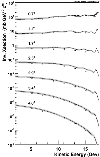
Figure 1: Proton invariant triple differential cross section measured (open square) in the $p+Be\rightarrow p+X$ at 19 Gev/c reaction allaby compared with the fitted parametrization as a function of the proton kinetic energy and for different production angles : 0.7^o, 1.1^o (scaled by a factor $10^{-1}$), 1.7^o ($\times 10^{-2}$), 2.3^o ($\times 10^{-3}$), 2.9^o ($\times 10^{-4}$), 3.4^o ($\times 10^{-5}$) , 4.0^o ($\times 10^{-6}$).

II.2 Atmospheric and Geomagnetic model

The model used to simulate the atmosphere is the MSISE-90 model available from MSISE which describes the temperature and densities in the earth’s atmosphere from ground to thermospheric altitudes.

The geomagnetic model used in this version of the simulation is IGRF9 IGRF which is the ninth generation of a mathematical model of the Earth’s main field and its annual rate of change (secular variation) adopted by the International Association of Geomagnetism and Aeronomy (IAGA).

II.3 Particle propagation

Each particle is propagated in the geomagnetic field and interacts with nuclei of the local atmospheric density. The particles trajectory is built by numerically integrating the equation of motion using the fifth order Runge Kutta method with adaptive step-size control from ref recipes . At each step of the propagation, in addition to the three coordinates and the three components of the momentum, the grammage crossed by the particle is computed. This allows the integration step size to be adapted to the local value of the atmosphere density and then insure a smooth penetration in the atmosphere and a precise calculation of the interaction probability and of the ionization energy loss, and the latter be computed for each step along the trajectory.

Every secondary particles are processed the same way as their parent particle, leading to the generation of an atmospheric cascade, more or less extensive, for each event. Nucleons, pions and kaons are produced for each interaction with their respective triple differential cross sections.

II.4 Particle interaction and secondary production

The cross sections used to produce secondary particles ($p$, $n$, $\pi^{\pm}$, $K^{\pm}$) are a very important input in the calculation, and the main source of uncertainty in the atmospheric flux estimation. In the present approach the particle production cross sections are obtained from fits to the data using an approach based on the Kalinovsky-Mokhov-Nikitin (KMN) parametrization of the inclusive hadronic cross sections kali . In the present work, a wide set of experimental data have been used to constrain the parameters of a modified KMN analytical formula Cross . The set of data included in the fits have been selected to cover as far as possible, the kinematics of interest for atmospheric secondary particles production. An interest of this method is that together with the best fit parameter set for each reaction channel, the errors on the parameters can also be estimated.

An illustrative example is shown on figure 1 with the comparison between the data from allaby ($p+\textrm{Be}\rightarrow p+X$ at 19 Gev/c) and the fit results (solid line). For all the studied samples of each reaction channel, the reduced $\chi^{2}$ obtained from fits were found larger than 1, typically between 1 and 5. This could be expected since the statistical and systematic errors on the cross section measurements are usually approximate or poorly known. To account for this uncertainty, a scale factor on the experimental error equal to 1/$\sqrt{\chi^{2}}$ has been included to evaluate the 95% confidence interval on the cross sections. This procedure is strictly valid only in case of purely statistical errors. It is thus not completely satisfying from this point of view but it should be rather conservative however. The gray band on the figure corresponds to this 95% confidence interval obtained for the proton production cross section (from the overall proton data analysis).

The obtained confidence intervals on the cross sections were then used to compute the uncertainty on the secondary particles flux, and ultimately, on the neutrino flux.

For the proton induced kaon production and the pion induced pion production the original KMN parametrizations were used kali . These cross sections are less critical since their contribution to the final neutrino flux are rather small, namely less than 25% and 5% respectively up to 30 GeV incident energy.

II.5 Particle decay

In the simulation, the ($\nu,\bar{\nu},e^{\pm}$) spectra from muon decay, were generated according to the Fermi theory, and the muon polarization was taken into account as in the previous work by the authors. For the kaon decay, the Dalitz plot distribution given in pdg04 was used.

II.6 Variance reduction techniques

To increase the efficiency of the simulation several techniques could be used to reduce the variance of the estimator produced by the simulation vrt . The technique used here was the important sampling method which consists simply of increasing arbitrarily the incident flux of particles, where the latter produce secondaries which contribute dominantly to the final differential flux to be evaluated, in a particular kinematical domain.

For instance, in the computation of the high energy neutrino flux, the high energy galactic flux of charged cosmic rays provides the dominant contribution. The natural abundance of this generic flux is extremely small however. The above mentioned technique is then used to get around this difficulty and the HE CR production probability is enhanced by a factor increasing the production yield of the secondaries of interest. The incident particle and all the particles produced in this event will then simply be weighted with the inverse enhancement factor used to boost the particle production. This weight is then taken into account when computing the estimator from the simulation (see next section).

Another classical use of this method is for computing the flux of a given particle in a given area at a given altitude. The primary particle flux generated vertically downwards around the zenith of the fiducial virtual detector area will have a much larger contribution to the calculated final flux, compared to CRs produced far away from this geographical region. In this case a natural way to improve the simulation efficiency is to increase production probability for particles generated near the detection region, and to correct for the induced bias by appropriate statistical weighting of the corresponding events, as described above.

The advantage of the method is that all contributing particles are taken into account in the generation process, none of them being excluded or neglected. A bad choice in the enhancement factor used to increase a certain class of primary particles would thus increase the variance of the estimators but it would not bias the results.

II.7 Particle detection and flux estimation

Each particle was traced by the program, and his history, trajectory parameters and kinematics, were recorded. The event file was then analyzed separately to generate the various distributions of interest.

To compare the simulated and the measured flux, a virtual surface of detection was defined at the detector altitude. It had to be large enough to ensure a large counting statistics and a precise estimation of the physics observables, but small enough to preserve the accuracy of the calculation. In practice the size of area for each computation was chosen to provide an accuracy below 1%.

The simulated differential particle flux is calculated ($m^{-2}\cdot s^{-1}\cdot sr^{-1}\cdot GeV^{-1}$) from the sum of the number of particles detected in the chosen area times, for each particle, the geometrical efficiency in the given particle direction of the considered experiment, times the weight obtained from the sampling method discussed in section II.6 to compensate the enhancement factor.

This latter number is then divided by the (local) surface of the particle collection area, the integral of detector acceptance over the full solid angle, energy bin size, and equivalent sampling time of the CR flux.

The equivalent sampling time of CR flux is obtained from the total event number generated in the simulation run(s) divided by the surface of the generation sphere times the integrated ($\cos\theta_{z}$ weighted) solid angle ($\pi$) times the energy integrated flux.

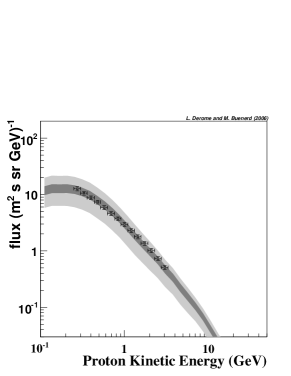
Figure 2: Open squares : Proton flux measured by the BESS experiment at mountain altitude 2770 m above sea level, data from BESS99 . Light gray band : 95 % confidence interval from the simulation. The estimation of the confidence interval includes only errors from the production cross sections. The dark gray band corresponds to the 95 % confidence interval obtained by fitting the cross section on atmospheric data (see section III.3.

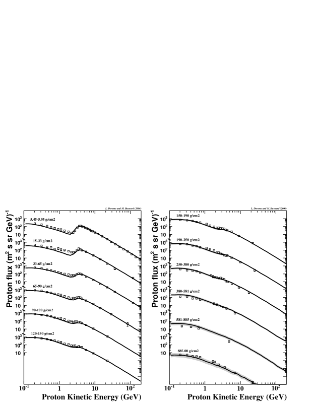
Figure 3: Proton flux measured by the Caprice experiment (open squares) for different altitudes in the atmosphere CAP98PROTON compqred with the flux estimated from the simulation (solid line). The light gray band shows the 95 % confidence interval from the simulation. This estimation of the confidence interval includes only errors from the production cross sections.

III Results

III.1 Proton flux in the atmosphere

The ability of the simulation to account for the proton production in the atmosphere can be probed by comparing the simulation results with the recent $p$ flux measurements performed by the CAPRICE experiment between sea level and high altitude ($\sim$ 40 km) CAP98PROTON , and by the BESS experiment at mountain altitude BESS99 .

Figure 2 shows the flux measured by BESS BESS99 compared to the calculated flux. The Bess measurements were performed at Mt Norikura, Japan (geographical location 36N,137.5E) at 2770 m of altitude above sea level (corresponding to an atmospheric depth of 742 g/cm2 ) in 1999.

The virtual detector area for this computation was chosen as the geographical region defined by $0.4<|\lambda_{CGM}|<0.6$ rad where $\lambda_{CGM}$ is the CGM latitude CGM , thus consisting of two bands (one in each hemisphere) centered on plus or minus the experiment CGM latitude (0.509 rad).

As in the measurements, the geometrical efficiency is set to one for zenithal angular range $\theta_{z}$ with $\cos\theta_{z}\geq 0.95$.

Figure 2 shows the confidence interval on the accuracy of the simulated flux (with a 95 % level). The estimation of the confidence interval includes only the error associated to the cross section and were computed using the confidence interval associated to the cross section parametrization (see section II.4). The large width of the confidence interval in this estimation is due to the large number of collisions between the primary particle and the detected proton at low altitude. Any uncertainty in the proton production cross section is then amplified by a large factor (approximatively 8 on the average, see BA03 ).

Figure 3 shows the flux measured by CAPRICE for different altitudes in the atmosphere during the 1998 flight from Fort Summer, N. M., (34.28 N, 105.14 W, CGM latitude 0.76 rad) CAP98PROTON and the corresponding simulation results.

The virtual detector area for this computation was chosen as the region defined by $0.74<|\lambda_{CGM}|<0.78$ rad. The geometrical efficiency used here was taken from CAP98PROTON to reproduce the detector acceptance. At high altitude, the effect of the geomagnetic cutoff is clearly observed in all spectra. At this CGM latitude the mean geomagnetic cutoff is 6 GeV for protons. Above the cutoff the flux is dominated by the primary cosmic component whereas below the geomagnetic cutoff the flux consists only of secondary protons produced by cosmic rays above the cutoff. The primary flux is increasingly absorbed in the atmosphere with the decreasing altitude, and the secondary component becomes dominant over the entire energy range.

The confidence interval of the calculated flux is seen to increase with the decreasing altitude, i.e., with the mean number of interactions as it could be expected BA03 . It can be observed that at low altitudes, the uncertainty of the simulation results (which includes only the production cross section uncertainties) is much larger than the uncertainty from the flux measurements. Therefore, the precise proton flux data at low altitudes can be used to constrain the parametrization of the secondary particles production more tightly and more accurately than the available nuclear data.

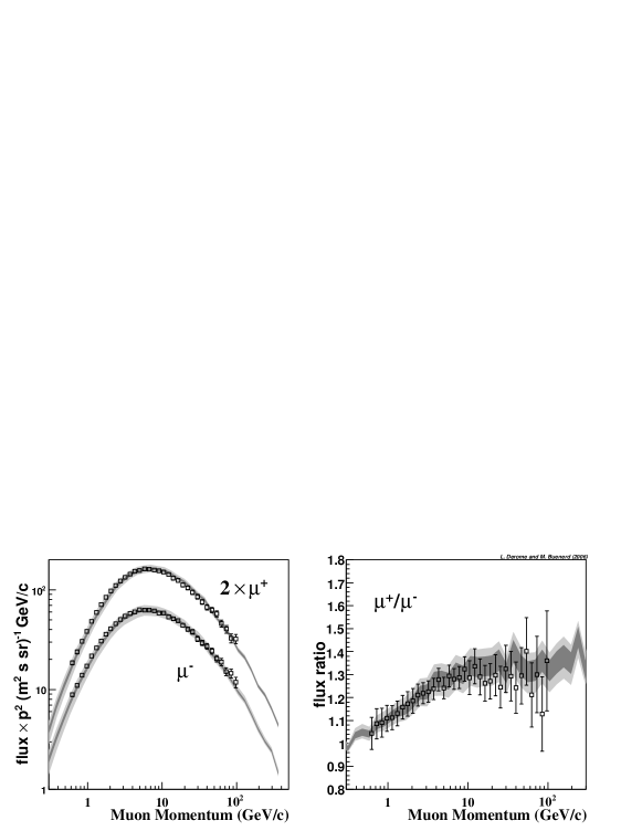
Figure 4: Open squares : Muon flux and muon flux ratio measured at Mt Norikura, Japan (location 36 ^oN,137.5 ^oE, altitude 2770 m above see level corresponding to a atmospheric depth of 742 g/cm2 ). Data from BessMuonMountain . The light gray band shows the 95 % confidence interval from the simulation. The estimation of the confidence interval includes only errors from the production cross sections. The dark gray band corresponds to the 95 % confidence interval obtained by fitting the cross section on atmospheric data (see text, section III.3).

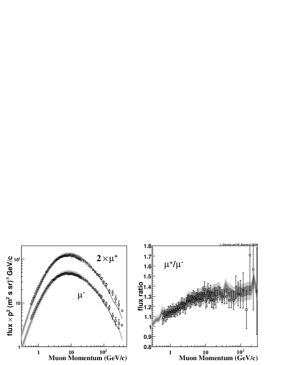
Figure 5: Open squares : Muon Flux and muon flux ratio in Tsukuba, Japan (location 36.2 ^oN,140.1 ^oE, altitude 30 m above sea level). The data are from BessMuonTsukuba . The light and dark gray bands are defined as in figure 4.

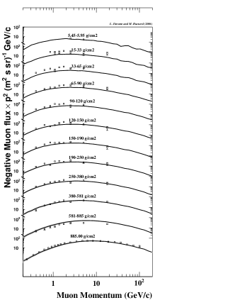
Figure 6: Positive and negative muon flux measured by the Caprice experiment for different altitudes in the atmosphere. The solid line shows the calculated flux and the light gray area corresponds to the 95% confidence interval.

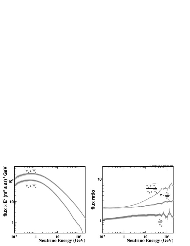
Figure 7: Neutrino flux (left) and Neutrino flux ratio (right) at the SK location average over $4\pi$. The light gray band corresponds to the 95 % confidence interval from the simulation. The estimation of the confidence interval includes only errors from the production cross sections. The dark gray band represents the 95 % confidence interval obtained by fitting the cross section on atmospheric data (see text, section III.3).

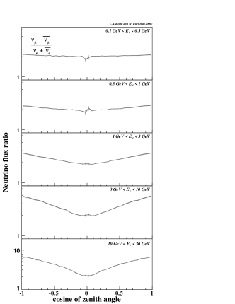
Figure 8: Zenith angle distributions and flavor ratio $(\nu_{\mu}+{\bar{\nu}_{\mu}})/(\nu_{e}+{\bar{\nu}_{e}})$ of the calculated neutrino flux around the Super-Kamiokande detector for five energy bin from 0.1 to 30 Gev. The light and dark gray bands are defined as in Fig. 7 (see text, section III.3).

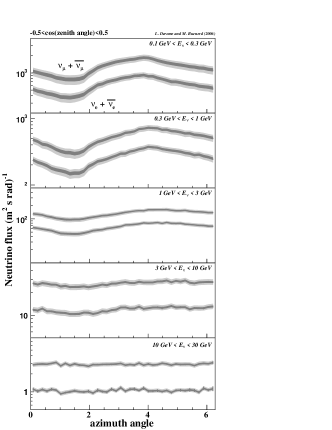
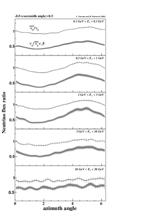
Figure 9: Azimuth angle distribution of the neutrino flux (left) and flavor ratios, $\nu_{e}/{\bar{\nu}_{e}}$ and ${\bar{\nu}_{\mu}}/{\nu_{\mu}}$ (right) at the SK detector location for five energy bins from 0.1 to 30 Gev. The light and dark gray bands are defined as in Fig. 7 (see text, section III.3).

III.2 Muon flux in the atmosphere

Atmospheric muons are produced in the same decay chain as neutrinos. Their spectra are thus an essential ground to probe the reliability of the neutrino flux calculated in the same framework. Several experiments, CAPRICE, HEAT, BESS, have made precise flux measurements at various altitudes in the atmosphere BessMuon2 ; BessMuonMountain ; BessMuonTsukuba ; Cap98Muon ; CapMuon ; HeatMuon which can be used for this purpose.

Figures 4 and 5 show the calculated positive and negative muon flux and the corresponding flux ratios compared with the data measured by the BESS experiment at mountain altitude (Mt Norikura, location 36N,137.5E, altitude 2770 m) BessMuonMountain and at sea level (Tsukuba, location 36.2 ^oN,140.1 ^oE, altitude 30 m) BessMuonTsukuba .

For these two calculations, the virtual detectors were chosen as the region defined by $0.4<|\lambda_{CGM}|<0.6$ rad at the experiment altitude, and with the geometrical efficiency set to one for zenithal angles $\theta_{z}$ with $\cos\theta_{z}\geq 0.98$.

The 95 % confidence interval is also shown on the figure. It includes the uncertainty originating from the parametrization of the secondary protons, neutrons and pions production cross sections. Note that for the muon charge ratio the uncertainty results only from the uncertainty on the pion production cross section.

Figure 6 shows the calculated positive and negative muon flux compared with the data measured by the CAPRICE experiment during the 1998 flight Cap98Muon at Fort Summer. A good agreement is found between data and the calculation for the positive and negative fluxes at different altitude going from the top of atmosphere to the ground level.

III.3 Use of atmospheric flux measurements to constrain hadron production cross sections

It is clearly seen on the figures 2 to 6 that, at least for the low altitude measurements, the statistical precision achieved by the atmospheric experiments is significantly better than the precision obtained from the simulation, taking into account the uncertainty on secondary particles production cross section. This results was obtained although all the relevant available nuclear data have been collected to constrain the parametrized cross sections used in these calculations. Therefore, the atmospheric flux measurements are in this sense more accurate that the nuclear data.

In other works on neutrino flux calculations, the calculated atmospheric flux of charged particles, used to check the reliability of the calculations, were all based on existing hadronic Monte Carlo generator honda ; battistoni ; barr , whereas in the present approach, in account of the good accuracy of the available measurements, the atmospheric data flux can be used to constrain the hadronic cross sections to ultimately improve the final accuracy of the calculated neutrino flux.

In this work, the proton and muon measurements at the Mt Norikura altitude and the muon measurements in Tsukuba, from the Bess experiment, were used to constrain both the proton and pion production cross sections. The obtained 95 % interval of confidence is shown (dark gray) on figure 2,4 and 5. The reduced $\chi^{2}$ obtained from this fit was 4.7, and the same procedure as described in section II.4 was thus used to estimate the confidence interval. It must be noted that these fitted cross sections may absorb systematic errors originating from other sources, like the primary CR fluxes, although the uncertainty on the latter are much smaller than on the cross sections. However, this does not affect the ultimate improvement of the neutrino flux uncertainty, since the deduced interval of confidence accounts for both sources of uncertainty.

III.4 Neutrino flux at SuperKamiokande Location

The calculated energy distributions of the atmospheric neutrino flux around the SuperKamiokande (SK) detector have been computed with the same simulation program. A virtual detector center was defined at the SK geographical coordinates (36^oN,137^oE) with a size of 8^o in latitude and 18^o in longitude (or $\sim$900$\times$1600 km²). The virtual detector size has been chosen so as not to change the calculated flux by more than 1 %.

Figure 7 shows the average flux over the full $4\pi$ range of solid angle for $\nu_{\mu}+\bar{\nu}_{\mu}$ and $\nu_{e}+\bar{\nu}_{e}$ (left) and the flux ratio $\frac{\nu_{\mu}+\bar{\nu}_{\mu}}{\nu_{e}+\bar{\nu}_{e}}$, $\frac{\nu_{\mu}}{\bar{\nu}_{\mu}}$ and $\frac{\nu_{e}}{\bar{\nu}_{e}}$ (right). The light gray area represents the 95 % confidence level corresponding to the uncertainty due to the particle production cross sections inaccuracies. The uncertainty for the absolute neutrino flux is of the order of 10 % and, as expected, these error contributions are largely reduced for the ratio of flux $\frac{\nu_{e}}{\bar{\nu}_{e}}$ (insensitive to proton/neutron production cross sections) and for $\frac{\nu_{\mu}}{\bar{\nu}_{\mu}}$ (insensitive to proton/neutron production cross sections but also to pion production cross sections for low energy neutrinos) and vanished for the $\frac{\nu_{\mu}+\bar{\nu}_{\mu}}{\nu_{e}+\bar{\nu}_{e}}$ flux ratio (insensitive to proton/neutron and pion production cross sections). The dark gray band correspond to the 95 % confidence interval obtained by fitting the cross section on atmospheric data discussed in the section III.3. Using this method the uncertainty for the absolute flux is reduced to the order of 3 %.

The zenith angle distribution of the flux and of the flavor ratios are shown on figure 8.left for 5 energy bins between 0.1 and 30 GeV. At low energy the zenith angle distribution displays an enhancement for directions close to horizontal, in qualitative agreement with lip1 . This enhancement originates from the isotropisation of the neutrino flux resulting from cosmic ray showers. It is expected to be maximum for a purely isotropic neutrino emission and nil for a perfectly collimated neutrino production. The maximum is then naturally obtained for the lowest energy bin (about twice the downward or upward going flux out of the horizontal plane). It is decreasing with the increasing energy. At low energy the zenith angle distribution for downward and upward neutrinos, outside the $\cos\theta=0$ peak, is approximatively flat, this isotropy naturally originating from the CR isotropy. The small structures observed arise from geomagnetic effects on the primary flux. At high energies the distributions become sensitive to the muon decay probability which depends on the muon pathlength in the atmosphere and on its energy. As expected the $|\cos\theta_{z}|$ dependence is becoming steeper with the increasing energy. The effect is enhanced for electronic neutrino which originate exclusively from muon decay. This is shown on figure 8.right where the flavor ratio $(\nu_{\mu}+{\bar{\nu}_{\mu}})/(\nu_{e}+{\bar{\nu}_{e}})$ is seen to depend on the zenith angle, especially for high energy neutrinos, for the same reason as given previously.

On these figures, the light gray area represents the 95% confidence level corresponding to the particle production uncertainty. Here again we see that the uncertainty is reduced at high energy, this is mainly due to the decrease of the mean number of interactions between the primary cosmic ray impinging the atmosphere and the final neutrino detection. As in figure 7, for the flavor ratio $(\nu_{\mu}+{\bar{\nu}_{\mu}})/(\nu_{e}+{\bar{\nu}_{e}})$ the error contributions from particle production uncertainty vanished. The dark gray band represents the 95 % confidence interval obtained by fitting the cross section on atmospheric data as described in section III.3.

The azimuth angle distribution of the flux and of the flavor ratios are shown on figure 9 for 5 energy bins between 0.1 and 30 GeV. On this figure northward and westward going particles correspond to azimuth angles 0, $\frac{\pi}{2}$ respectively. The non-flatness of the low energy bin originates from the geomagnetic cutoff on primary cosmic rays lip2 . The east-west (EW) effect of the primary flux (more eastward going than westward going cosmic rays) results in a EW asymmetry in the produced secondary particles and then in the neutrino flux at low energy. With the increasing energy, neutrinos are increasingly produced in atmospheric showers initiated by higher energy cosmic rays which are less and less sensitive to the geomagnetic cutoff (the cosmic ray flux becomes isotropic at a rigidity of 60 GV). This results in the simulated azimuthal distribution becoming flat for the last energy bin in figure 9.left (neutrino energy between 10 Gev and 30 Gev).

For the azimuth angle distributions of the flavor ratios (figure 9.right), it can be noted that the $\nu_{e}/{\bar{\nu}_{e}}$ ratio is strongly EW asymmetric while the opposite is observed for the $\nu_{\mu}/{\bar{\nu}_{\mu}}$ ratio. The $(\nu_{\mu}+\bar{\nu_{\mu}})/(\nu_{e}+\bar{\nu_{e}})$ ratio (not shown) is found to be almost structureless at all latitudes. This additional EW asymmetry featured by the $\nu_{e}/{\bar{\nu}_{e}}$ and $\nu_{\mu}/{\bar{\nu}_{\mu}}$ ratio can be explained by the muon bending in the geomagnetic field lip2 . In the production chain $p\rightarrow\pi^{+}\rightarrow\mu^{+}\nu_{\mu}\rightarrow\nu_{e}{\bar{\nu}_{\mu}}$, the muon will propagate with the same bending as the proton one. An enhancement of EW effect originating from the geomagnetic cutoff is then expected for the neutrino $\nu_{e}$ and ${\bar{\nu}_{\mu}}$ produced in the $\mu^{+}$ decay. In the $p\rightarrow\pi^{-}\rightarrow\mu^{-}{\bar{\nu}_{\mu}}\rightarrow\nu_{\mu}{\bar{\nu}_{e}}$ production chain, the muon will propagate with the opposite bending and a reduction of the EW asymmetry is expected for the $\mu^{-}$ decay products $\nu_{\mu}$ and ${\bar{\nu}_{e}}$. This explains the EW features seen in the $\nu_{e}/{\bar{\nu}_{e}}$ and the $\nu_{\mu}/{\bar{\nu}_{\mu}}$ ratio. In addition, because muonic neutrinos are also produced in the pion decay, the EW asymmetry is found to be higher for $\nu_{e}/{\bar{\nu}_{e}}$ than for ${\bar{\nu}_{\mu}}/\nu_{\mu}$. These results confirm the qualitative prediction from lip2  :

$$A_{\bar{\nu}_{e}}<A_{\nu_{\mu}}<A_{\bar{\nu}_{\mu}}<A_{\nu_{e}}$$

where $A$ stands for the neutrino EW asymmetry.

In figure 9 the light and dark gray area represents respectively the 95 % confidence level corresponding to the particle production cross section uncertainty and the 95 % confidence interval obtained by fitting the cross section on atmospheric data as described in section III.3. The uncertainty are largely reduced for the ratio of flux $\frac{\nu_{e}}{\bar{\nu}_{e}}$ (insensitive to the proton/neutron production cross sections) and for $\frac{\bar{\nu}_{\mu}}{\nu_{\mu}}$ (insensitive to proton/neutron production cross sections but also to pion production cross sections for low energy).

IV Summary and conclusion

A full three-dimensional simulation has been used to compute the secondary particles production in the atmosphere. In these calculations the statistics of the simulated sample has been significantly increase with respect to our previous work, resulting in a negligible contribution of the statistical uncertainty. The dominant error then appeared to come from the uncertainty on the particle production cross sections. In this work this systematic uncertainty has been studied quantitatively.

The simulation has been used to reproduce the atmospheric measurements of the proton and muon flux, in order to test the reliability of the calculations. These atmospheric measurements, in account of their good accuracy, were also used to constrain the secondary particle production cross sections, which experimental values from direct measurements on accelerators were of lesser accuracy.

The results for the absolute neutrino fluxes and their zenithal and azimuthal angular distributions together with the flavor ratio of these flux at the Super-Kamiokande location, have been presented. The high statistics accumulated allowed to investigate the detailed structure of these distribution and to discuss them. The uncertainty of the calculations has been estimated. It has been shown first, that this uncertainty is at the level of 10 % for the absolute flux, and second that it can be reduced to the level of 3 % by using the atmospheric data on the muon and proton flux to constrain the production cross sections. These results provide an accurate basis for the comprarison to future experimental data.