Measuring Flexion

Abstract

We describe practical approaches to measuring flexion in observed galaxies. In particular, we look at the issues involved in using the Shapelets and HOLICs techniques as means of extracting 2nd order lensing information. We also develop an extension of HOLICs to estimate flexion in the presence of noise, and with a nearly isotropic PSF. We test both approaches in simple simulated lenses as well as a sample of possible background sources from ACS observations of A1689. We find that because noise is weighted differently in shapelets and HOLICs approaches, that the correlation between measurements of the same object is somewhat diminished, but produce similar scatter due to measurement noise.

1. Introduction

1.1. Motivation

Flexion has recently been introduced as a means of measuring small scale variations in weak gravitational lens fields (Goldberg & Bacon, 2005; Bacon, Goldberg, Rowe & Taylor, 2006, hereafter BGRT). Rather than simply measuring the ellipticities of arclets, this technique aims to measure the “arciness” and “skewness” (collectively referred to as “flexion”) of a lensed image. Flexion is a complementary approach to shear analysis in that it uses the odd moments (3rd multipole moments, for example) to compute local gradients in a shear field. BGRT have discussed how flexion may be used to identify substructure in clusters, to normalize the matter power spectrum on sub-arcminute scales via “cosmic flexion” (as an analog to cosmic shear), and to estimate the ellipticity of galaxy-galaxy lenses. As a practical application, flexion has already been used to measure galaxy-galaxy lensing (Goldberg & Bacon, 2005), and is presently being used in cluster reconstruction (Leonard et al., in preparation).

However, there have been several difficulties in the estimation of flexion on real objects. First, the flexion inversion is difficult to describe, contains an enormous number of terms, and thus, is rather daunting to code. Secondly, there has been little discussion of the explicit effects of PSF convolution or deconvolution. Finally, unlike shear, there has, until recently, been no simple form to even approximate what the “flexion” is.

The remainder of this paper will thus be a practical guide to measuring flexion in real images. We begin, below, by reminding the reader of the basic terms involved in flexion analysis. In § 2, we review shapelet decomposition, and discuss some of the issues involved in using shapelets to measure flexion. In § 3, we discuss a new, conceptually simpler, form of flexion analysis developed by Okura et al. (2006), which uses moments, rather than basis functions to measure flexion. They call their technique Higher Order Lensing Image’s Characteristics, or HOLICs. We refine the HOLICs approach somewhat, and develop a KSB (Kaiser, Squires, & Broadhurst, 1995)-type approach using a Gaussian filter to perform an inversion, as well as describe a technique for PSF deconvolution. In § 4, we discuss comparisons of the two techniques using simulated lenses and simulated PSFs. In § 5, we compare shapelets and HOLICs inversions on HST images. Finally, in § 6, we discuss the implications of this study.

In Appendix A, we also present the explicit HOLICs inversion matrix, so the reader can write his/her own code. He/she need not do so, however, as all codes discussed herein are available from the flexion webpage.

1.2. Flexion

What is flexion? Conceptually, flexion represents local variability in the shear field which expresses itself as second-order distortions in the coordinate transformation between unlensed and lensed images:

$$\beta_{i}\simeq A_{ij}\theta_{j}+\frac{1}{2}D_{ijk}\theta_{j}\theta_{k},$$ (1)

with

$$D_{ijk}=\partial_{k}A_{ij}\ ,$$ (2)

where $\partial_{k}$ is shorthand for $\partial/\partial x_{k}$. Here, ${\bf A}$ is the normal deprojection operator:

$${\bf A}=\left(\begin{array}[]{cc}1-\kappa-\gamma_{1}&-\gamma_{2}\\ -\gamma_{2}&1-\kappa+\gamma_{1}\end{array}\right)\ ,$$ (3)

and thus, the second term on right in equation (1) represents the flexion signal. ${\bf D}$ may be written as:

$$D_{ij1} = \left(\begin{array}[]{cc}-2\gamma_{1,1}-\gamma_{2,2}&\ \ -\gamma_{2,1}\\ -\gamma_{2,1}&\ \ -\gamma_{2,2}\end{array}\right),$$ (6)

$$D_{ij2} = \left(\begin{array}[]{cc}-\gamma_{2,1}&\ \ -\gamma_{2,2}\\ -\gamma_{2,2}&\ \ 2\gamma_{1,2}-\gamma_{2,1}\end{array}\right).$$ (9)

These distortions create asymmetries in a lensed image – a skewness and a bending, depending on the values of individual coefficients. Irwin & Shmakova (2005;2006) describe a similar lensing analysis technique in which the elements of ${\bf D}$ are referred to as “Catenoids” and “Displacements.”

BGRT describe an inversion whereby one can estimate the individual components, and thus measure two “flexions”:

$${\cal F}\equiv\partial^{\ast}\gamma$$ (10)

$${\cal G}=\partial\gamma$$ (11)

where $\partial$ is the complex derivative operator:

$$\partial=\partial_{1}+i\partial_{2}\ .$$ (12)

Figure 1 is reproduced from BGRT and shows the effect of a first or second flexion on a circular source.

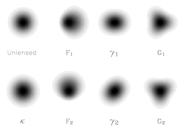
Figure 1.— From Bacon, Goldberg, Rowe & Taylor, 2006. The lensed images corresponding to pure first or second flexion, shear, or magnification.

An object with first flexion, ${\cal F}$, appears skewed, while an object with second flexion, ${\cal G}$, appears arced, especially if the image has an induced shear as well. The first flexion has an $m=1$ rotational symmetry, and thus behaves like a vector. In particular, it is a direct tracer of the gradient of the convergence:

$${\cal F}_{1}{\bf i}+{\cal F}_{2}{\bf j}=\nabla\kappa$$ (13)

where ${\cal F}_{1}$ is the real component and ${\cal F}_{2}$ is the imaginary part (as with the second flexion and, as the standard convention, with shear).

The second flexion has an $m=3$ rotational symmetry, though unlike the first flexion, it has no simple physical interpretation like that of the first flexion. It is, however, roughly proportional to the local derivative of the magnitude of the shear. A more complete discussion of flexion formalism can be found in BGRT.

2. Shapelets Decomposition

2.1. Review of Shapelets

Measurement of flexion ultimately requires very accurate knowledge of the distribution of light in an image. The shapelets (Refregier 2003; Refregier & Bacon 2003) method of image reconstruction decomposes an image into 2D Hermite polynomial bases:

$$f({\bf\theta})=\sum_{n,m}{\cal B}_{nm}({\bf\theta})f_{nm}\ .$$ (14)

This technique has a number of very natural advantages. In the absence of a PSF, all shapelet coefficients will have equal noise. Moreover, the basis set is quite localized (Hermite polynomials have a Gaussian smoothing filter), and thus is ideal for modeling galaxies. Furthermore, the generating “step-up” and “step-down” operators for the Hermite polynomials are simply combinations of the $x_{i}$, and $\partial_{i}$ operators.

Refregier (2003) shows that if we decompose a source image, $f$, into shapelet coefficients, the transformation to a lensed image may be expressed quite simply as:

$$f^{\prime}=(1+\kappa\hat{K}+\gamma_{j}\hat{S}_{j})f$$ (15)

where the various lensing operators are:

$$\hat{K} = 1+\frac{1}{2}\left(\hat{a}_{1}^{\dagger 2}+\hat{a}_{2}^{\dagger 2}-\hat{a}_{1}^{2}-\hat{a}_{2}^{2}\right)$$

$$\hat{S}_{1} = \frac{1}{2}\left(\hat{a}_{1}^{\dagger 2}-\hat{a}_{2}^{\dagger 2}-\hat{a}_{1}^{2}+\hat{a}_{2}^{2}\right)$$

$$\hat{S}_{2} = \frac{1}{2}\left(\hat{a}_{1}^{\dagger}\hat{a}_{2}^{\dagger}-\hat{a}_{1}\hat{a}_{2}\right)\ ,$$ (16)

$\hat{a}^{\dagger}$ and $\hat{a}$ are the normal step-up and step-down operators, and the subscript refers to the directional component of the coefficient (i.e. 1 for the first or x-component, and 2 for the second, or y-component). Note that in the weak field limit, these operators indicate that power will be transferred between coefficients with indices $|\Delta n|+|\Delta m|=2$, which preserves symmetry as well as keeping the image representation in shapelet space compact.

In Goldberg & Bacon (2005), similar (albeit more complicated) transforms were found relating the derivatives of shear. We will not reproduce the full second order operators here, as they are written in full in the earlier work, but we will point out some key features. First, some of the elements in the operators have an explicit dependence on the (unlensed) quadrupole moments of the light distribution. This is due to a relatively subtle effect not present in shear analysis. Since the flexion signal is asymmetric, the center of brightness in the image plane will no longer necessarily correspond to the center of brightness in the source plane, and since the shapelet decomposition is performed around the center of light, we need to correct for this.

Most important, though, is the fact that second order lensing terms yield transfer of power between indices with $|\Delta n|+|\Delta m|=$ 1 or 3. To second order, then, a lensed image can be expressed as:

$$f^{\prime}=(1+\kappa\hat{K}+\gamma_{j}\hat{S}_{j}+\hat{S}_{ij}^{(2)}\gamma_{i,j})f\ .$$ (17)

Flexion analysis assumes (as does shear analysis) that the intrinsic flexion is random, and thus all “odd” (defined as n+m) moments are expected to be zero. Thus, from a set of shapelet coefficients, a best estimate for the flexion signal may be found via $\chi^{2}$ minimization, where:

$$\chi^{2}\equiv\left[\mu_{n_{1}m_{1}}-f_{n_{1}m_{1}}+(\gamma_{i}\hat{S}_{i}^{(1)}+\gamma_{i,j}S_{ij}^{(2)})\overline{f}_{n^{\prime}_{1}m^{\prime}_{1}}\right]V^{-1}_{n_{1}m_{1}n_{2}m_{2}}\left[(\mu_{n_{2}m_{2}}-f_{n_{2}m_{2}}+(\gamma_{i}\hat{S}_{i}^{(1)}+\gamma_{i,j}S_{ij}^{(2)})\overline{f}_{n^{\prime}_{2}m^{\prime}_{2}}\right],$$ (18)

$V_{n_{1}m_{1}n_{2}m_{2}}$ is the covariance matrix of the shapelet coefficients, and $\mu_{nm}$ is the “unlensed” estimate of a shapelet coefficient. For odd modes, this is zero. For even modes, the relative effect of shear is typically much smaller than the intrinsic ellipticity of an image, thus it makes sense to set $\mu_{nm}=f_{nm}$.

2.2. Effective Estimation of the Flexion

Though the form looks quite complicated, conceptually, computing the flexion is very straightforward. A simplified pipeline may be written as follows:

1. Generate a catalog of objects and, for each, excise an isolated postage stamp.

2. Compute the shapelet coefficients of the postage stamp.

3. Deconvolve the postage stamp with a known PSF kernel.

4. Compute the transformation matrices associated with each of the four flexion operators, solve the $\chi^{2}$ minimization (equation 18) for $\gamma_{i,j}$, and estimate the flexion.

We discuss each of these steps in turn below. The data used for this analysis was taken using HST and the Advanced Camera for Surveys, and in the particular context of cluster lensing. In this context, the galaxies in which we are interested are potentially blended with much larger and brighter foreground objects. We discuss the specific properties of our data catalog in § 5, but many of the issues involved are quite generic.

2.2.1 Catalog Generation and Postage Stamp Cutout

The first step in the process, the generation of a catalog and postage stamps seems quite straightforward. For some datasets, such as the SDSS (York et al. 2000), the data release includes an atlas of pre-cut postage stamps. For other applications, such as in relatively shallow galaxy-galaxy or cosmic shear/flexion studies, fields will be relatively uncrowded and thus simple application of widely used packages such as SExtractor (Bertin & Arnouts, 1996) can be used.

When fields are crowded, however, and contain a wide range of brightnesses and sizes, the catalog generation becomes more complicated. It has been noted by Rix et al. (2004) that in general, a single set of SExtractor parameters is insufficient for detection of all the objects of interest within an image; setting the source detection threshold too low will result in excessive blending near bright objects, whereas a high threshold results in a failure to detect fainter sources. Rix et al. describe a two-pass strategy for object detection and deblending involving an initial (“cold”) pass to identify large, bright objects, followed by a lower-threshold (“hot”) pass to pick up dimmer objects. Their final catalog consists of all the objects detected in the cold run, plus any objects detected in the hot run that do not lie within the isophotal area of any object detected in the first pass.

This technique works well to prevent spurious deblending by SExtractor in images in which there is significant substructure. However, when dealing with crowded fields (such as clusters of galaxies) the largest problem in catalog generation is excessive blending of sources, particularly in the central region. To remedy this, we use a modified version of this hot/cold technique. Our method consists of a primary SExtractor run to detect only the brightest objects. In a lensing field, especially in a lensing cluster, these bright objects will tend to be the lenses. Making use of the RMS maps generated during this SExtractor run, we mask out the bright objects by setting the pixel values to background noise, and thus simulate an emptier field.

We then run SExtractor on the masked image, using a much lower detection threshold, to create a catalog of background objects. Since shape estimation including both flexion and shear have a minimum of 10 degrees of freedom, we require at least 10 connected pixels above the detection threshold, though in reality, we are unlikely to be able to get a reliable measurement from an image with fewer than 15 included pixels. We then discard all objects for which reliable shape estimates cannot be found.

For each remaining object, a postage stamp is generated. Ideally, this should identify any neighboring objects and mask them out (by setting their pixel values equal to background noise). Our postage stamp code also identifies objects which are blended by using a friends-of-friends algorithm to find sets of connected pixels that are a certain threshold (typically 2-3$\sigma$ for the stacked images described below) above the background. If there is any overlap between the object of interest and another object within the field of the postage stamp, we consider the source to be excessively blended and exclude it from further analysis.

2.2.2 Shapelet Decomposition

Shapelets can be an extremely compact representation of an individual image. However, in reality, they are a family of basis functions. There is a characteristic scaling parameter, $\beta$, which represents the width of the Gaussian kernel in the basis function Hermite polynomials:

$${\cal B}_{nm}({\bf\theta})\propto\exp\left(-\frac{\theta_{1}^{2}+\theta_{2}^{2}}{2\beta^{2}}\right)\ .$$ (19)

In principle, while all values of $\beta$ will yield an orthonormal basis set, some values produce a dramatically faster reconstruction in terms of the number of coefficients required to reach convergence. Moreover, in reality we don’t want to reconstruct all details in an image. Structure on the individual pixel scale may simply represent noise.

From a practical perspective, our goal is to optimize selection of $\beta$, and the maximum coefficient index, $n_{max}$. Refregier (2003) suggests the following parameters:

$$\beta\simeq\sqrt{\theta_{min}\theta_{max}}$$

$$n_{max}\simeq\frac{\theta_{max}}{\theta_{min}}-1\ ,$$ (20)

where $\theta_{min}$ and $\theta_{max}$ represent the minimum and maximum scales of image structure, respectively.

R. Massey (private communication) has found that rather than performing overlap integrals to solve for the shapelet coefficients (as was done, for example, in the analysis of Goldberg & Bacon 2005), the ideal approach is to do a $\chi^{2}$ minimization of the reconstructed image with the original postage stamp. This may seem complicated, and it is. Fortunately, a shapelets package is available in IDL at the shapelets webpage.

For our sample of co-added, background-subtracted, HST ACS images of Abell 1689, we find that $\theta_{min}=0.4$ pixels and $\theta_{max}=1.8\sqrt{a^{2}+b^{2}}$ give good shapelet reconstructions, where $a$ and $b$ are the semi-major and semi-minor axes of the galaxy as measured by SExtractor. However, it is important to note that these parameters are somewhat dependent on the noise level in the images.

For a sky-limited sample, we have found that the optimal choice of $\theta_{min}$ scales approximately linearly as the ratio of the flux to the RMS sky noise. We have looked at this scaling in a sample of galaxies detected with ACS (and which we describe in greater detail below), each of which was imaged in 4 frames. Prior to stacking of these frames, we found that $\theta_{min}=0.75$ produced low $\chi^{2}$ and convergence with small values of $n_{max}$. After stacking, $\theta_{min}=0.4$ was required. This makes sense, since the noisier our image, the more prone we might otherwise be to fitting complex polynomials to what is, essentially, noise.

Roughly, the processing time for a decomposition scales as $\theta_{max}^{4}$, as $\theta_{max}$ determines both the postage stamp size and the maximum order of the shapelet decomposition. Due to the high resolution of our images, we encountered a number of objects for which $n_{max}$ was so large that the decomposition time became prohibitive. We opted to re-grid images with $n_{max}>50$ into larger pixels by taking the mean of the pixel values in square bins, the size of which is determined by $binsize=n_{max}/50$. This number was rounded up for objects with $50<n_{max}\leq 75$.

A flexion measurement is then carried out using the $\chi^{2}$ minimization technique described previously. However, we have found that truncating the shapelet series prior to the flexion measurement yields a more accurate and robust measure of the flexion than using the full series. Excluding the higher order shapelet modes avoids contamination of the flexion signal by small scale substructure and by noise (particularly in dimmer objects). We exclude all shapelet modes with $n>n_{max}/5$ in our flexion measurement. This effectively increases $\theta_{min}$ to 2 pixels, without affecting the accuracy of the reconstruction.

2.2.3 PSF Deconvolution

One of the complications in measuring properties of lensed images is that, in practice, they are convolved with a PSF:

$$f({\bf\theta})=\int d^{2}\theta^{\prime}P({\bf\theta-\theta^{\prime}})f^{(0)}({\bf\theta})\ .$$ (21)

In principle, the PSF can be estimated through measurement of stars, but in deep, small-field, high galactic-latitude observations, stars may be scarce, and thus PSF estimation may rely partly on numerical analysis of the instrument (e.g. the Tiny Tim algorithm, Krist, J. 1993).

In reality, though, this should rarely be an issue. Estimations of the PSF flexion from Tiny Tim yield values of $\sigma_{aF,psf}\simeq 7\times 10^{-4}$. This represents the maximum induced flexion which can arise from convolution with the PSF, and is still several orders of magnitude lower than the scatter in intrinsic flexion of galaxies.

We are not surprised by this since, for example, PSF distortions arising from variable sizes in chips is likely to scale as the variation in PSF ellipticity. In ACS, chip distortions produce ellipticities of order $1\%$, and vary on scales of 100’s of pixels, producing an induced flexion of $\sim 10^{-4}\ pix.^{-1}$. From the ground, the atmospheric distortions are expected, on average, to be even more isotropic.

There is another reason to suppose that PSF flexion contributions will be unimportant. In shear measurements, the PSF ellipticity typically varies smoothly and somewhat symmetrically around the center of a field, mimicking (or partially reversing) the overall behavior of the expected shear field. Since flexion probes smaller scale effects, the induced flexion by the PSF will, on average, cancel out.

This is not to say that we cannot deal with PSF flexion inversion. Refregier (2003) describes an explicit deconvolution algorithm (see also Refregier and Bacon 2003, and references therein). In shapelet space, equation (21) can be re-written as:

$$f_{nm}=\sum_{n^{\prime}m^{\prime}n^{\prime\prime}m^{\prime\prime}}C_{nmn^{\prime}m^{\prime}n^{\prime\prime}m^{\prime\prime}}P_{n^{\prime}m^{\prime}}f^{(0)}_{n^{\prime\prime}m^{\prime\prime}}$$ (22)

Where $C_{nmn^{\prime}m^{\prime}n^{\prime\prime}m^{\prime\prime}}$ is the 2-dimensional convolution tensor:

$$C_{nmn^{\prime}m^{\prime}n^{\prime\prime}m^{\prime\prime}}(\gamma,\alpha,\beta)=2\pi(-1)^{n+m}i^{n+m+n^{\prime}+m^{\prime}+n^{\prime\prime}+m^{\prime\prime}}\int d^{2}{\bf x}{\cal B}_{n^{\prime\prime}m^{\prime\prime}}({\bf x}/\gamma){\cal B}_{n^{\prime}m^{\prime}}({\bf x}/\alpha){\cal B}_{nm}({\bf x}/\beta)\ ,$$ (23)

and $\alpha$, $\beta$ and $\gamma$ are the characteristic scales of $f^{(0)}$, $P$ and $f$, respectively. We may then define a PSF convolution matrix as:

$$P_{nmn^{\prime}m^{\prime}}\equiv\sum_{n^{\prime\prime}m^{\prime\prime}}C_{nmn^{\prime}m^{\prime}n^{\prime\prime}m^{\prime\prime}}P_{n^{\prime\prime}m^{\prime\prime}}\ .$$ (24)

If only low order terms in the convolution matrix are included, it may be inverted to perform a deconvolution via:

$$f^{(0)}_{nm}=\sum_{n^{\prime}m^{\prime}}(P^{-1})_{nmn^{\prime}m^{\prime}}f_{n^{\prime}m^{\prime}}\ .$$ (25)

This provides a good estimate of the low order coefficients, but high order information is lost. An alternative inversion scheme involves fitting the observed galaxy coefficients using a $\chi^{2}$ minimization scheme. Refregier and Bacon (2003) note that the $\chi^{2}$ scheme may be more robust numerically, and can take full account of variations in the noise characteristics across an image (although it is strictly only valid in the case of Gaussian noise). It is this scheme that is implemented in the shapelets IDL software.

2.2.4 Flexion Inversion

If the shapelet coefficients are statistically independent (as they will be in the absence of an explicit PSF deconvolution), formal inversion of the flexion operator is quite straightforward. Under these circumstances, we also have the benefit that the measurement error for each moment is identical (see Refregier 2003 for discussion).

Noting that, in most galaxies, the coefficients corresponding to the $n+m=$even moments will be much larger than the odd moments (and, indeed, upon random rotations, the latter will necessarily average to zero) we can dramatically simplify equation (18). First, we define the susceptibility of each odd moment as:

$$\Delta f_{n^{\prime}m^{\prime},ij}=\hat{S}^{(2)}_{ij}f_{nm}$$

where $f_{nm}$ represents all of the “even” coefficients, and $n^{\prime}m^{\prime}$ represents all of the odd coefficients. Thus, we wish to solve for the relation:

$$\sum_{n^{\prime}m^{\prime}}(f_{n^{\prime}m^{\prime}}-\gamma_{i,j}\Delta f_{n^{\prime}m^{\prime},ij})^{2}=min.$$ (26)

where the first term is taken directly from measurement. Taking the derivatives and rearranging, we find:

$$\sum_{n^{\prime}m^{\prime}}f_{n^{\prime}m^{\prime}}\Delta f_{n^{\prime}m^{\prime},ij}=\gamma_{i,j}\sum_{n^{\prime}m^{\prime}}(\Delta f_{n^{\prime}m^{\prime},ij}\Delta f_{n^{\prime}m^{\prime},i^{\prime}j^{\prime}})$$ (27)

which can readily be inverted to solve for $\gamma_{i,j}$.

In practice, however, there are a number of issues which must be considered. First, if the PSF or pixel scale are relatively large compared to the minimum resolution scale of an image then many of the high-order moments returned by shapelets decomposition will, in fact, not have any information. Thus, the above inversion will yield a systematic underestimate of the true image flexion. Above, we describe a truncation which minimizes this effect.

While the flexion inversion is, at its core, linear algebra, it involves an enormous number of terms. We have thus provided an inversion code for shapelets estimates of flexion along with examples on the flexion webpage.

3. HOLICs Analysis

3.1. Higher Order Moments

Okura et al. (2006) recently related flexion directly to the 3rd moments of observed images. This is a significant extension of flexion, and very much along the lines of Goldberg & Natarajan’s (2002) original work which talked about “arciness” in terms of the measured octopole moments. Throughout our discussion, we will use the notation:

$$Q_{ij}=\frac{1}{F}\int(\theta_{i}-\overline{\theta_{i}})(\theta_{j}-\overline{\theta_{j}})f({\bf\theta})d^{2}{\bf\theta}$$ (28)

to refer, in this case, to the unweighted quadrupole moments, with all higher moments being defined by exact analogy. In this context, $F$ refers to the unweighted integrated flux.

They define the complex terms:

$$\zeta\equiv\frac{(Q_{111}+Q_{122})+i(Q_{112}+Q_{222})}{\xi}$$ (29)

and

$$\delta\equiv\frac{(Q_{111}-3Q_{122})+i(3Q_{112}-Q_{222})}{\xi}$$ (30)

where

$$\xi\equiv Q_{1111}+2Q_{1122}+Q_{2222}\ .$$ (31)

These terms are collectively referred to as HOLICs.

If a galaxy is otherwise perfectly circular (i.e. no ellipticity), and in the absence of noise, then the HOLICs may be directly related to estimators of the flexion (subject to an unknown bias of $1-\kappa$). Namely:

$${\cal F}\simeq\frac{4\zeta\xi}{9\xi-6(Q_{11}^{2}+Q_{22}^{2})}$$ (32)

$${\cal G}\simeq\frac{4\delta}{3}$$ (33)

where the latter term in the denominator of ${\cal F}$ does not appear in the Okura et al. analysis. Bacon and Goldberg (2005) show that a flexion induces a shift in the centroid proportional to the quadrupole moments. In order to correctly invert the HOLICs, this term needs to be incorporated explicitly. The simplicity of the extra term results from an approximation of near circularity.

The beauty of this approach is that it gives us a very intuitive feel for what flexion means in an observational way. We thus introduce the term “skewness” to the intrinsic properties of a galaxy as measured from equation (32) whether or not the galaxy is otherwise circular, and whether or not it is lensed. The skewness may be thought of as the intrinsic property, much as the “ellipticity” is the intrinsic property related to the “shear.” Likewise, the intrinsic property associated with equation (33) will be referred to as the “arciness.”

In reality, however, equations (32) and (33) are not sufficient to perform a flexion estimate even if a galaxy has an ellipticity of only a few percent. Okura et al provide a general relationship between estimators for flexion and HOLICs, though the relation is best expressed in matrix form:

$${\cal M}\left(\begin{array}[]{c}{\cal F}_{1}\\ {\cal F}_{2}\\ {\cal G}_{1}\\ {\cal G}_{2}\end{array}\right)=\left(\begin{array}[]{c}\zeta_{1}\\ \zeta_{2}\\ \delta_{1}\\ \delta_{2}\end{array}\right)$$ (34)

where ${\cal M}$ is a $4\times 4$ matrix consisting of elements proportional to sums of $Q_{ijkl}$ and $Q_{ij}Q_{kl}$, the former of which can be found by explicitly expanding the expressions in Okura et al., and the latter of which is again derived from the shift in the centroid. For the convenience of the reader, we write out the explicit form of ${\cal M}$ in Appendix A.

It may be seen by examining the elements of ${\cal M}$ why this inversion must be done explicitly for even mildly elliptical sources. For fully circular sources, it may be seen by inspection that ${\cal M}$ is diagonal. However, when a source has an ellipticity even as small as $10\%$, it can be shown that $|M_{11}|\simeq|M_{12}|$, and thus equations (32) and (33) are no longer even approximately correct.

3.2. Gaussian Weighting with HOLICs

The application of the HOLICs technique would be trivial if there were no measurement noise. In the presence of noise, and especially, when the sky dominates, measurement of unweighted moments is inherently quite noisy. In a case where we are measuring the 3rd and 4th moments, it is even more so.

Kaiser, Squires & Broadhurst (1995; see also a nice review by Bartelmann & Schneider, 2001) developed perhaps the most comprehensive approach to dealing with the second moments (the ellipticity) with noisy observing, and with a (potentially anisotropic) PSF.

Our approach is similar. We have only worked with a Gaussian window thus far, but the approach is generalizable for any circularly symmetric weighting. We thus define a window function:

$$W({\bf\theta})=\frac{1}{2\pi\sigma_{W}}\exp\left(-\frac{\theta_{1}^{2}+\theta_{2}^{2}}{2\sigma_{W}^{2}}\right)$$ (35)

where the origin is taken to be the center of light, and the integral is normalized to unity. Further, we define the weighted moments as, for example:

$$\hat{Q}_{11}=\frac{1}{\hat{F}}\int(\theta_{1}-\overline{\theta_{1}})^{2}f({\bf\theta})W({\bf\theta})d^{2}{\bf\theta}\ .$$ (36)

We can thus redefine all HOLICs and moments similarly. We have found through experimentation (see below) that for a sky noise limited source, a reasonable value of $\sigma_{W}$ is 1.5 times the half-light radius.

If we were to simply replace all elements in ${\cal M}$, $\zeta$, and $\delta$ from equation (34) with their weighted counterparts we would not get an unbiased estimate of the flexion. There are two corrections. One has to do with the fact that centroid shift will differ from the unweighted case to the weighted case. Consider an extreme scenario in which the window width is arbitrarily small and in which the unlensed image was circularly symmetric with a peak at the center. In that case, the centroid will essentially remain at the center (peak brightness) even if the unweighted moments shift.

Thus, compared to the unweighted moments, the centroid will shift:

$$\Delta\overline{\theta}_{l}=\frac{\sum_{ijk}D_{ijk}\hat{Q}_{ijkl}}{\sigma_{W}^{2}}$$ (37)

where we have used the explicit fact that for a Gaussian:

$$\frac{dW({\bf\theta})}{d\theta_{i}}=-\frac{\theta_{i}}{\sigma_{W}^{2}}W({\bf\theta})\ ,$$ (38)

The other correction has to do with the fact that though lensing preserves surface brightness, it does not preserve total flux. This is normally related by the Jacobian of the coordinate transformation. However, when considering a window function, we need consider that transformation explicitly:

$$W(\beta)d^{2}\beta=\left|\frac{\partial\beta}{\partial\theta}\right|W(\beta)d^{2}\theta$$ (39)

as used by Okura et al. (2006), and where we have simply multiplied both sides by the factor $W(\beta)$. In this context, ${\bf\beta}$ refers to the image coordinate in the source plane. Ignoring the terms proportional to shear (which cannot be directly addressed by this method at any rate), we have the approximate relation:

$$W(\beta)\simeq W(\theta)+\frac{1}{2}D_{ijk}\theta_{i}\theta_{j}\frac{dW}{d\theta_{k}}$$ (40)

or, as we have already asserted:

$$W(\beta)\simeq W(\theta)-\frac{1}{2}D_{ijk}\frac{\theta_{i}\theta_{j}\theta_{k}}{\sigma_{W}^{2}}W(\theta)\ .$$ (41)

Note that the latter term contains an odd number of position elements, and thus, coupling to the generating equations for $\zeta$ and $\delta$ produces contributions of $6^{th}$ moments in ${\cal M}$:

$$\Delta\hat{Q}_{ijk}=-\frac{1}{2}D_{lmn}\frac{\hat{Q}_{ijklmn}}{\sigma_{W}^{2}}\ ,$$ (42)

which, in turn, must be corrected for.

We may thus say that:

$$\hat{\cal M}={\cal M}(\hat{Q}_{ij},...)+\Delta{\cal M}\ ,$$ (43)

where the latter expression can also be found in Appendix A.

3.3. PSF Correction in HOLICs

As with our discussion of shapelets, above, we must also consider PSF deconvolution in our HOLICs pipeline. We define the PSF function in equation (21), and all unweighted moments of the PSF are denoted by $P_{ij}$, etc. In principle, because of the higher signal-noise of the PSF, the unweighted moments are easier to estimate than the moments of the detected image. While we argued, above, that the induced flexion from a PSF is likely to be small, it is still the case, as with shear, that the PSF will reduce the measured flexion. Let’s first consider the case in which we were able to measure the unweighted moments of both the PSF and the observed image. It is straightforward to show that:

$$Q_{ij}=Q_{ij}^{(0)}+P_{ij}\ .$$ (44)

Thus may be computed via the relation:

$$Q_{ij}=\frac{1}{F}\int\theta_{i}\theta_{j}f^{(0)}(\theta^{\prime})P(\theta-\theta^{\prime})d^{2}\theta d^{2}\theta^{\prime}$$ (45)

Making the substitution,

$$\theta^{\prime\prime}=\theta-\theta^{\prime}$$ (46)

yields

$$Q_{ij}=\frac{1}{F}\int(\theta_{i}^{\prime}\theta_{j}^{\prime}+\theta_{i}^{\prime\prime}\theta_{j}^{\prime\prime}+\theta_{i}^{\prime}\theta_{j}^{\prime\prime}+\theta_{i}^{\prime\prime}\theta_{j}^{\prime})f^{(0)}(\theta^{\prime})P(\theta^{\prime\prime})d^{2}\theta^{\prime}d^{2}\theta^{\prime\prime}$$ (47)

It is straightforward to show that this yields equation (44).

Similarly, it may be shown that:

$$Q_{ijk}=Q_{ijk}^{(0)}+P_{ijk}\ .$$ (48)

However,

$$Q_{1111}=Q_{1111}^{(0)}+P_{1111}+6Q_{11}^{(0)}P_{11}\ ,$$ (49)

with a similar expression for $Q_{2222}$, and

$$Q_{1122}=Q_{1122}^{(0)}+P_{1122}+Q_{11}^{(0)}P_{22}+Q_{22}^{(0)}P_{11}$$ (50)

provided we assume the PSF is nearly circular.

If we further look only at nearly circular sources, then we may estimate the flexion using the forms in equations (32) and (33). Again, assuming unweighted moments, and zero PSF and intrinsic flexion we find:

$$\tilde{{\cal F}}_{i}={\cal F}_{i}\frac{9\xi^{(0)}-6(Q^{(0)2}_{11}+Q^{(0)2}_{22})}{9\xi-6(Q_{11}^{2}+Q_{22}^{2})}$$ (51)

Where ${\cal F}_{i}$ is an unbiased estimate of the flexion, and $\tilde{{\cal F}}_{i}$ is the estimated flexion if one does not include the correction for the PSF. However, the normalization constant may be estimated directly from combinations of the PSF 2nd and 4th moments, and the unweighted moments of the image. Since this term represents something like the overall radial profile of the source, the unweighted moments can be estimated even under noisy conditions.

Similarly, the second flexion may be estimated as:

$$\tilde{{\cal G}}_{i}={\cal G}_{i}\frac{\xi^{(0)}}{\xi}$$ (52)

Though we have derived these relations for a nearly circular source, we have found they provide a good correction even when the PSF and intrinsic image size are comparable, and when ellipticities for the source image are $\varepsilon\simeq 0.2$.

4. Simulated Lensing

Which approach is better, shapelets or HOLICs? From a signal perspective, the shapelets technique is better. It is designed to provide optimal weighting and return optimal signal-noise. Moreover, as described above, inversion of the PSF is a straightforward and well-designed process. In the absence of noise, the two techniques produce very similar results.

On the other hand, the HOLICs technique has several practical advantages, especially for large surveys. For one, the HOLICs code is typically much faster than shapelets. For an N pixel image, the HOLICs technique is an ${\cal O}(N)$ calculation, whereas the shapelets is ${\cal O}(N^{2})$. Additionally, some values of $\beta$ produce very bad reconstructions, and hence, minimization of $\chi^{2}$ can be time-consuming and may not converge to a minimum.

As a simple test, we created images with brightness profiles of:

$$I(r)\propto\exp[-(r/r_{0})^{n}]$$ (53)

and though we found similar results for a reasonable range of exponents, the results presented below are for $n=1.5$. We have used a constant source ellipticity, typical of those observed in the field, $\varepsilon=0.2$, and had measurement errors which were dominated by sky brightness. In each case, we had no intrinsic arciness or skewness (that is, the flexion of the unlensed objects were zero), since our aim was to measure the response of each of the estimators to lensing.

We then artificially lensed each of our simulated images, added sky noise, and measured the flexion using both the HOLICs and shapelets techniques. The noise is fixed throughout this discussion, as is the strength of the flexion signal. It is clear, however, that all relevant signal-noise values will scale linearly with the strength of the lensing signal and inversely with sky noise.

4.1. Optimzing the HOLICs Scale Factor

Our first questions is, what is the optimal value of $C_{W}$, such that:

$$\sigma_{W}=C_{W}\times r_{half-light}\ ?$$ (54)

Ideally, we would like an unbiased estimator of the flexion which also has very little scatter. It is clear that the larger the value of $C_{W}$, the larger the scatter will be (in general), since we will be measuring more and more of the noisy sky. However, the smaller the $C_{W}$, the less accurate will be our measure of the real shape of the galaxy. Figure 2 bears this out. There is an optimal value of $C_{W}$ around 1.5, which reflects a balance between minimizing measurement errors as well as any measurement bias inherent in the technique.

Figure 2.— The fractional error in the mean (left panel) and standard deviations (right panel) of the measured, simulated 1st flexion (solid), and 2nd flexion (dashed), as discussed in the text.

With shapelets, we find a systematic underestimate of 11% in the first flexion, and an overestimate of 12% in the second flexion. We find a scatter of about 12% in both. This is very similar in magnitude to the results found by an “optimal” HOLICs analysis.

4.2. Correlation of HOLICs and Shapelets Measurement Error

Since both HOLICs and shapelets give similar measurement errors at fixed sky noise, it is worth considering whether we expect measurement errors between the two techniques to be correlated. Even in these idealized circumstances, uncorrelated errors would mean that there is significant information in the images which is not being used. In Fig. 3, we show the correlation in uncertainty between our $C_{W}=1.5$ HOLICs estimates, and our shapelets estimates.

Figure 3.— Scatter plots showing the fractional random errors in first flexion (left panel), and second flexion (right panel) from HOLICs (x-axis), and shapelets (y-axis). The correlation is quite high for 1st flexion, with a Pearson correlation coefficient of $\rho_{F}=0.86$, and $\rho_{G}=0.23$.

For the first flexion, in particular, the correlation is quite high, with a Pearson correlation coefficient of $0.86$. The correlation in measurements of the second flexion is much lower, with $\rho_{G}=0.23$. Why don’t they have perfect correlation? The two techniques weight various components of the signal (and thus, the noise) differently, and therefore have a slightly different response to the noise.

This general trend is borne out with observed objects as well, in which we will see much higher correlation between measurements of the first flexion than the second flexion between the two techniques.

4.3. PSF Deconvolution

Finally, we can simulate PSF deconvolution. Using a Gaussian PSF with a characteristic size somewhat larger than the intrinsic image (the correction factor described in equation 51 is 2.7), we distorted and then recovered the flexion estimates from images of increasing intrinsic ellipticity. This analysis is done in the absense of sky noise, and thus any errors in shape recovery represent a systematic effect. We show the fractional errors in measurement of the first and second flexion in Figure 4. Since it is possible to estimate the systematic error for a combination of measured shear and PSF shape, it is advisable to those wishing to make high-precision flexion measurements to take this empirical correction into account.

Figure 4.— The fractional error in the recovered flexion estimate using a Gaussian PSF with scale of order the size of the intrinsic image. Note that errors increase with increasing ellipticity, but produce reasonable errors ($\sim 25\%$) in both the 1st flexion (solid line), and 2nd flexion (dashed). No measurement noise is included in these calculations, and thus, this result represents the systematic error in measurement.

We find that, despite the fact that the PSF correction is based on an assumption of circularity, it continues to produce a good result even if the image has an intrinsic ellipticity as high as 0.3.

5. Measurement of Flexion on HST Images

5.1. Sample Selection and Pipeline

We also compare the two approaches to flexion inversion on real objects. Our data consists of 4 HST ACS cosmic-ray rejected (CRJ) images of Abell 1689 using the F625W WFC filter (hereafter “R-band”). Each image was taken by H. Ford during HST Cycle 11, and has an exposure time between 2300-2400 seconds. The observations are described in detail in Broadhurst et al. (2005).

Using the SWarp software package , these four images were co-added to create a single “full” R-band image. We also generated 2 independent “split” images for comparison purposes by combining only two of the original images. The images are background-subtracted, aligned and re-sampled, then projected into subsections of the output frame using a gnomonic (or tangential) projection, and combined using median pixel values.

Each image undergoes a primary SExtractor run designed to detect only the foreground objects (cluster members and known stars). This detection is carried out using the cross-correlation utility in SExtractor, which allows us to specify the locations of the foreground objects. Our foreground object catalog was generated using a combination of spectroscopically confirmed cluster members (Duc et al. 2002), and identification by eye of foreground objects that were later confirmed as such by use of the NASA/IPAC Extragalactic Database (NED), as well as clearly identifiable stars in the field. These objects are then masked out as described previously, and a second SExtractor run carried out.

A catalog of objects is then generated, using only those objects that were detected in both of the split R-band images. We measure the flexion in our catalog objects using both the truncated shapelets method (described above) and the HOLICs approach, and then compare the measurements by computing Pearson correlation coefficients between the different estimates in the full image. We also compute correlation coefficients between measurements taken using the same technique in the two split images. This gives us an estimate of the robustness of the measurement technique.

When computing the correlation coefficients, we include only objects with $a>3$ pixels, and consider only the brightest half of our catalog objects. In order to exclude extreme or erroneous measurements, we require $(a|\cal{F}|)<$ 0.2 and $(a|\cal{G}|)<$ 0.5.

5.2. Results

Figure 5 shows a comparison of the HOLICs and shapelets estimates of flexion in the full image. Both $\cal{F}$ and $\cal{G}$ have a positive correlation, with a Pearson correlation coefficient of 0.17 for $\cal{F}$ and 0.12 for $\cal{G}$. Additionally, both methods yield similar standard deviations for both first and second flexion.

This is what we expected from our simulated results above. Clearly, if flexion represents any real signal, the two techniques should be correlated, and, as we showed in our simulated results, the correlation in first flexion is higher than in second flexion. But the correlation in our measured results is lower than in the simulated ones. Why? In part, this is due to a relatively noisy field. We’ve found that selections on brighter magnitudes and larger objects improves the correlation somewhat. In part, however, this is due to what we mean by “flexion.” Recall that the shapelets and HOLICs analysis of flexion involve weighting different modes in different ways. Real, unlensed, galaxies will have odd modes which are not necessarily correlated in a simple or obvious way. Lensing, of course, produces a significant correlation, and thus, a population of significantly lensed objects (for which the majority of the flexion is due to lensing) would be expected to have a more correlated flexion. This is similar to the case with weak shear analysis in that the S/N from a typical object is usually less than 1.

We can test this hypothesis directly by comparing the measurements in the split images and estimating the flexion in both using the same technique. Any discrepancies between the two ought to be the result of photon noise rather than intrinsic complexity in the structure of the 3rd moments.

Figure  6 shows a comparison of the HOLICs measurements made on each of the split images. These measurements are well correlated: the Pearson correlation coefficient here is 0.37 for $\cal{F}$ and 0.23 for $\cal{G}$. In Figure  7, we see a comparison of the shapelets measurements in these images, which appear to be more strongly correlated (particularly for $\cal{F}$). The Pearson correlation coefficients here are 0.58 for $\cal{F}$ and 0.18 for $\cal{G}$.

Figure 5.— A scatter plot of the values of ${\cal F}$ and ${\cal G}$ as measured using a truncated shapelets technique and a HOLICs (or moments) method in the full stacked image.

Figure 6.— A comparison of HOLICs measurements of ${\cal F}$ and ${\cal G}$ in the split images.

Figure 7.— Truncated shapelets measurements of ${\cal F}$ and ${\cal G}$ in the split images

As motivated above, most of the “noise” in our measurements comes from the intrinsic distribution of flexion within our sample. Indeed, using the HOLICs approach, we find:

$$\sigma_{a|F|+Noise}=0.05$$ (55)

$$\sigma_{a|G|+Noise}=0.08$$ (56)

The distribution function may be seen in Fig. 8. Note that this result includes noise. However, we may estimate the relative effect of photon noise on this scatter by using correlation between frames. That is:

$$\sigma_{a|F|}=\sqrt{\rho}\sigma_{a|F|+Noise}$$ (57)

And thus, we find that our best estimate of the intrinsic scatter in first flexion is:

$$\sigma_{a|F|}=0.03$$ (58)

(as found in Goldberg & Bacon 2005), and

$$\sigma_{a|G|}=0.04\ .$$ (59)

Figure 8.— The histogram of $a|{\cal F}|$ and $a|{\cal G}|$ for our measured sample. This represents an estimate of the intrinsic distribution of flexion among our source population.

The combination $a|{\cal F}|$ represents a dimensionless term, and thus is independent of distance.

It should also be noted that since these measurements are taken within a cluster, the signal is included as well, and one might question whether it is reasonable to estimate the intrinsic variability of flexion from lensed images. The intrinsic scatter in flexion was originally measured in Goldberg & Bacon (2005), and we merely confirm the result here. However, this is a reasonable thing to do, as flexion drops off much more quickly than shear, and thus, even within a rich cluster, the flexion signal is dominated by individual galaxies. Even at a separation of $1^{\prime\prime}$, the flexion from even a very massive $300km/s$ galaxy on an $a=0.4^{\prime\prime}$ source is about 0.05, approximately the level of the intrinsic flexion. Such separations are relatively rare, however.

6. Discussion

We have endeavored to present a detailed guide to measuring flexion in real observations, with a focus on space-based imaging. In the process, we have taken a look at two different approaches to measuring flexion: shapelets and HOLICs, with an eye toward which approach is “better.” From an idealized perspective of maximal signal-noise, the answer is simple. Shapelets produces a mode-by-mode comparison which optimally averages to produce a unique estimate of flexion. However, this result is complicated somewhat in two limits: blending, which affects larger objects, and PSF convolution, which affects smaller ones.

When images are blended, it is clear that we benefit by giving extra weighting to those pixels near the center of the the object. In that sense, HOLICs can be said to produce more robust results. Likewise, despite an explicit PSF deconvolution algorithm, applying the flexion inversion using shapelets results in inclusion of small scale power which has been blended away through the atmosphere or instrument. We have discussed, above, how this might be alleviated by only using relatively low order modes from the reconstruction in the estimate of flexion. However, doing so comes at the expense of some (but by no means all), of the signal-noise advantage from shapelets. Indeed, even using a relatively truncated form of the shapelets analysis still produced greater correlation between independent images of the same objects, and thus, cleaner estimates of the flexion.

However, one complication in the shapelets analysis is producing a good shapelets decomposition in the first place. While R. Massey’s shapelet code comes with an optimization routine to find the best fit scaling parameter, $\beta$, the shapelet decomposition runs several orders of magnitude slower than HOLICs. For very large lensing fields, this may prove a significant limitation, and thus, HOLICs provides a fast, physically motivated, reasonably reliable alternative.

Appendix A Expanded Coefficients for HOLICs Analysis of Flexion

In equation (34), we state that the flexion may be solved via inversion of the relation:

$$y={\cal M}x$$ (A1)

where $x$ is a vector of the desired flexion estimators, and $y$ is the measure of the 3rd order HOLICs. Here, we show the explicit form of M.

$$M_{11} = \frac{1}{4}(9+8\eta_{1})-\frac{33Q_{11}^{2}+14Q_{11}Q_{22}+Q_{22}^{2}+20Q_{12}^{2}}{4\xi}$$

$$M_{12} = 2\eta_{2}-\frac{32Q_{12}Q_{22}+32Q_{11}Q_{12}}{4\xi}$$

$$M_{13} = \frac{1}{4}(2\eta_{1}+\lambda_{1})-\frac{3Q_{11}^{2}-2Q_{11}Q_{22}-Q_{22}^{2}-4Q_{12}^{2}}{4\xi}$$

$$M_{14} = \frac{1}{4}(2\eta_{2}+\lambda_{2})-\frac{2Q_{11}Q_{12}}{\xi}$$

$$M_{21} = 2\eta_{2}-\frac{32Q_{12}Q_{22}+32Q_{11}Q_{12}}{4\xi}$$

$$M_{22} = \frac{1}{4}(-8\eta_{1}+9)-\frac{Q_{11}^{2}+14Q_{11}Q_{22}+20Q_{12}^{2}+33Q_{22}^{2}}{4\xi}$$

$$M_{23} = \frac{1}{4}(-2\eta_{2}+\lambda_{2})-\frac{-2Q_{12}Q_{22}}{/\xi}$$

$$M_{24} = \frac{1}{4}(2\eta_{1}-\lambda_{1})-\frac{(Q_{11}^{2}+4Q_{12}^{2}+Q_{11}Q_{22}-3Q_{22}^{2})}{4\xi}$$

$$M_{31} = \frac{1}{4}(10\eta_{1}+7\lambda_{1})-\frac{3(11Q_{11}^{2}-10Q_{11}Q_{22}-Q_{22}^{2}-20Q_{12}^{2})}{4\xi}$$

$$M_{32} = \frac{1}{4}(-10\eta_{2}+7\lambda_{2})-\frac{3(8Q_{11}Q_{12}-32Q_{12}Q_{22})}{4\xi}$$

$$M_{33} = \frac{3}{4}-\frac{3(-2Q_{11}Q_{22}+Q_{11}^{2}+Q_{22}^{2}+4Q_{12}^{2})}{4\xi}$$

$$M_{34} = 0$$

$$M_{41} = \frac{1}{4}(10\eta_{2}+7\lambda_{2})-\frac{3(32Q_{11}Q_{12}-8Q_{12}Q_{22})}{4\xi}$$

$$M_{42} = \frac{1}{4}(10\eta_{1}-7\lambda_{1})-\frac{3(Q_{11}^{2}+20Q_{12}^{2}+10Q_{11}Q_{22}-11Q_{22}^{2})}{4\xi}$$

$$M_{43} = 0$$

$$M_{44} = \frac{3}{4}-\frac{3(-2Q_{11}Q_{22}+Q_{11}^{2}+Q_{22}^{2}+4Q_{12}^{2})}{4\xi}$$ (A2)

where, as defined in Okura et al. (2006), we use:

$$\eta\equiv\frac{(Q_{1111}-Q_{2222})+2i(Q_{1112}+Q_{1222})}{\xi}$$ (A3)

$$\lambda\equiv\frac{(Q_{1111}-6Q_{1122}+Q_{2222})+4i(Q_{1112}-Q_{1222})}{\xi}$$ (A4)

Note that $\eta=0$ and $\lambda=0$ for all circularly symmetric distributions and even those with no ellipticity but with flexion.

If we apply a Gaussian weighting with width, $\sigma_{W}$, to our moment measurements, then ${\cal M}$ should be computed using the weighted moments. In addition, the following terms must be added:

$$\Delta M_{11} = \frac{-3Q_{111111}-6Q_{111122}-3Q_{112222}+3Q_{22}Q_{1122}+9Q_{11}Q_{1111}+6Q12Q_{1112}+9Q_{11}Q_{1122}+6Q_{12}Q_{1222}-3Q_{22}Q_{1111}}{4\xi\sigma_{W}^{2}}$$

$$\Delta M_{12} = \frac{-3Q_{111112}-6Q_{111222}-3Q_{122222}+3Q_{22}Q_{1112}+9Q_{11}Q_{1222}+3Q_{22}Q_{1222}+6Q_{12}Q_{1122}+9Q_{11}Q_{1112}+6Q_{12}Q_{2222}}{4\xi\sigma_{W}^{2}}$$

$$\Delta M_{13} = \frac{-Q_{111111}+2Q_{111122}+3Q_{112222}-3Q_{22}Q_{1122}+3Q_{11}Q_{1111}+2Q_{12}Q_{1112}-9Q_{11}Q_{1122}-6Q_{12}Q_{1222}+Q_{22}Q_{1111}}{4\xi\sigma_{W}^{2}}$$

$$\Delta M_{14} = \frac{-3Q_{111112}-2Q_{111222}+Q_{122222}+6Q_{12}Q_{1122}+9Q_{11}Q_{1112}-3Q_{11}Q_{1222}+3Q_{22}Q_{1112}-Q_{22}Q_{1222}-2Q_{12}Q_{2222}}{4\xi\sigma_{W}^{2}}$$

$$\Delta M_{21} = \frac{-3Q_{111112}-6Q_{111222}-3Q_{122222}+6Q_{12}Q_{1122}+3Q_{11}Q_{1112}+9Q_{22}Q_{1112}+3Q_{11}Q_{1222}+9Q_{22}Q_{1222}+6Q_{12}Q_{1111}}{4\xi\sigma_{W}^{2}}$$

$$\Delta M_{22} = \frac{-3Q_{111122}-6Q_{112222}-3Q_{222222}+6Q_{12}Q_{1112}+3Q_{11}Q_{2222}+6Q_{12}Q_{1222}+9Q_{22}Q_{1122}+3Q_{11}Q_{1122}+9Q_{22}Q_{2222}}{4\xi\sigma_{W}^{2}}$$

$$\Delta M_{23} = \frac{-Q_{111112}+2Q_{111222}+6Q_{122222}-6Q_{12}Q_{1122}+Q_{11}Q_{1112}+3Q_{22}Q_{1112}-3Q_{11}Q_{1222}-9Q_{22}Q_{1222}+2Q_{12}Q_{1111}}{4\xi\sigma_{W}^{2}}$$

$$\Delta M_{24} = \frac{-3Q_{111122}-2Q_{112222}+Q_{222222}+9Q_{22}Q_{1122}+3Q_{11}Q_{1122}-Q_{11}Q_{2222}+6Q_{12}Q_{1112}-2Q_{12}Q_{1222}-3Q_{22}Q_{2222}}{4\xi\sigma_{W}^{2}}$$

$$\Delta M_{31} = \frac{-3Q_{111111}+6Q_{111122}+9Q_{112222}-9Q_{22}Q_{1122}+9Q_{11}Q_{1111}-18Q_{12}Q_{1112}+9Q_{11}Q_{1122}-18Q_{12}Q_{1222}-9Q_{22}Q_{1111}}{4\xi\sigma_{W}^{2}}$$

$$\Delta M_{32} = \frac{-3Q_{111112}+6Q_{111222}+9Q_{122222}-9Q_{22}Q_{1112}+9Q_{11}Q_{1222}-9Q_{22}Q_{1222}-18Q_{12}Q_{1122}+9Q_{11}Q_{1112}-18Q_{12}Q_{2222}}{4\xi\sigma_{W}^{2}}$$

$$\Delta M_{33} = \frac{-Q_{111111}+6Q_{111122}-9Q_{112222}+9Q_{22}Q_{1122}+3Q_{11}Q_{1111}-6Q_{12}Q_{1112}-9Q_{11}Q_{1122}+18Q_{12}Q_{1222}-3Q_{22}Q_{1111}}{4\xi\sigma_{W}^{2}}$$

$$\Delta M_{34} = \frac{-3Q_{111112}+10Q_{111222}-3Q_{122222}-18Q_{12}Q_{1122}+9Q_{11}Q_{1112}-3Q_{11}Q_{1222}-9Q_{22}Q_{1112}+3Q_{22}Q_{1222}+6Q_{12}Q_{2222}}{4\xi\sigma_{W}^{2}}$$

$$\Delta M_{41} = \frac{-9Q_{111112}-6Q_{111222}+3Q_{122222}+18Q_{12}Q_{1122}+9Q_{11}Q_{1112}-9Q_{22}Q_{1112}+9Q_{11}Q_{1222}-9Q_{22}Q_{1222}+18Q_{12}Q_{1111}}{4\xi\sigma_{W}^{2}}$$

$$\Delta M_{42} = \frac{-9Q_{111122}-6Q_{112222}+3Q_{222222}+18Q_{12}Q_{1112}+9Q_{11}Q_{2222}+18Q_{12}Q_{1222}-9Q_{22}Q_{1122}+9Q_{11}Q_{1122}-9Q_{22}Q_{2222}}{4\xi\sigma_{W}^{2}}$$

$$\Delta M_{43} = \frac{-3Q_{111112}+10Q_{111222}-3Q_{122222}+18Q_{12}Q_{1122}+3Q_{11}Q_{1112}-3Q_{22}Q_{1112}-9Q_{11}Q_{1222}+9Q_{22}Q_{1222}+6Q_{12}Q_{1111}}{4\xi\sigma_{W}^{2}}$$

$$\Delta M_{44} = \frac{-9Q_{111122}+6Q_{112222}-Q_{222222}+9Q_{22}Q_{1122}+9Q_{11}Q_{1122}-3Q_{11}Q_{2222}+18Q_{12}Q_{1112}-6Q_{12}Q_{1222}+3Q_{22}Q_{2222}}{4\xi\sigma_{W}^{2}}$$ (A5)

References

- (1) Bacon, D. J., Goldberg, D.M., Rowe, B.T.P. & Taylor, A.N., 2006, MNRAS 365, 414
- (2) Bartelmann, M. & Schneider, P., 2001, Physics Reports 340, 291
- (3) Bertin, E. & Arnouts, S., 1996, A&AS 117, 393
- (4) Broadhurst, T., et al. 2005, ApJ 621, 53
- (5) Duc, P. et al., 2002, AA 382, 60
- (6) Goldberg, D.M. & Bacon, D.J., 2005 ApJ 619, 741
- (7) Goldberg, D.M. & Natarajan , P. 2002, ApJ 564, 65
- (8) Irwin, J. & Shmakova, M., 2005, NewAR 49, 83
- (9) Irwin, J. & Shmakova, M., 2006, ApJ, 645, 17
- (10) Kaiser N., Squires G., Broadhurst T., 1995, ApJ, 449, 460.
- (11) Krist, J. 1993, ASPC 52, 536
- (12) Okura, Y., Umetsu, K., & Futamase, T., 2006, submitted to ApJ, http://xxx.lanl.gov/abs/astro-ph/0607288
- (13) Refregier, A., 2003, MNRAS 338, 35
- (14) Refregier, A. & Bacon, D.J., 2003, MNRAS 338 48
- (15) Rix, H. et al., 2004, ApJS 152, 163
- (16) York, D.G. et al. 2000, AJ, 120, 1579