Evolution of Hii regions in hierarchically structured molecular clouds

Abstract

We present observations of the H 91$\alpha$ recombination line emission towards a sample of nine Hii regions associated with 6.7-GHz methanol masers, and report arcsecond-scale emission around compact cores. We derive physical parameters for our sources, and find that although simple hydrostatic models of region evolution reproduce the observed region sizes, they significantly underestimate emission measures. We argue that these findings are consistent with young source ages in our sample, and can be explained by existence of density gradients in the ionised gas.

1 Introduction

Ultracompact (UC) Hii regions are pockets of ionised hydrogen that form around massive stars in the earliest stages of their evolution. Together with massive bipolar outflows, strong far infrared emission by dust, and the presence of molecular masers, they are indicative of massive star formation in its earliest stages. The simple model of Hii region evolution [1978] does not explain many of their observed properties, such as the frequent occurrence of non-spherical morphologies and the lifetime paradox. This lifetime problem, first noted by Wood & Churchwell [1989], is that the number of observed UC Hii regions exceeds that predicted from their dynamical expansion timescales by two orders of magnitude, given the accepted massive star formation rate in the Galaxy. A number of modifications and enhancements to the basic model have been suggested, including the work of Dyson et al. [1995], Hollenbach et al. [1994], Tenorio-Tagle [1979] and van Buren et al. [1990], Franco et al. [1990], Arthur & Lizano [1997], Keto [2003]. The thermal [1995a] and turbulent [1996] pressure confinement models are appealing due to their dependence on the ambient conditions observed to commonly exist in molecular clouds.

De Pree et al. [1995a] suggested thermal pressure confinement as an explanation of the lifetime paradox. They noted that when Wood & Churchwell proposed the lifetime problem in 1989, the molecular medium surrounding the UC Hii regions was thought to have temperatures $\sim 25$ K and densities $\sim 10^{5}$ cm^-3. More recent observations indicate T$\sim 100$ K and n$\sim 10^{7}$ cm^-3. The resulting 400$\times$ increase in thermal pressure limits the expansion of the Strömgren sphere. A weakness of this model, noted by Xie et al. [1996], is the exceedingly high emission measures that it predicts ($\sim 10^{10}$ $\mbox{pc~{}cm}^{-6}$), which are more than two orders of magnitude greater than the values typically observed.

Hierarchical density and temperature structures are known to exist within star-forming regions, with hot cores embedded in larger, less dense molecular clumps which themselves are within still larger and less dense molecular clouds. The densities decrease by approximately an order of magnitude in going from core to clump and again from clump to cloud [1994]. In a seminal work, Franco et al. [1990] showed that these density inhomogeneities are important for Hii region evolution. That the hierarchical structure of molecular clouds plays an important role in Hii evolution is supported by the marked similarity in the ionised and neutral gas density structures observed within molecular clouds [1996, 2002, 2003].

The large thermal molecular line and recombination line widths observed towards many UC Hii regions suggest that significant turbulent motions are present, probably of magnetic origin [1996]. This led Xie et al. [1996] to suggest that turbulent pressure is the dominant mechanism to restrict the expansion of an Hii region. In contrast to thermal pressure confinement, the assumed densities are lower, resulting also in lower emission measures. During much of the expansion phase, however, the turbulent pressure is expected to play a lesser role than thermal pressure in confining the Hii region. This is discussed briefly in section 4.1.1.

Icke [1979] investigated the formation of Hii regions in non-homogeneous media and was able to explain some non-spherical morphologies. Observational evidence obtained in the last decade, however, suggests that many Hii regions have compact cores within diffuse, arcminute-scale extended emission [1999, 2001]. Other sources exhibit this to a smaller degree — the so-called core-halo morphology; see Wood & Churchwell [1989] and Kurtz et al. [1994]. A study of the compact and extended radio continuum emission and radio recombination lines (RRLs) from eight Hii regions known to be associated with 6.7-GHz methanol masers has been undertaken. The RRL analysis is presented here, while details of the continuum observations can be found in Ellingsen, Shabala & Kurtz [2005] (hereafter ESK05). In section 2 we briefly outline our observations. The results are presented in section 3, and these are compared with a simple model in section 4. A discussion of our findings is presented in section 5.

2 Observations

Eight UC Hii regions with associated methanol maser emission were observed with the Australia Telescope Compact Array (ATCA) on 1999 July 10 and 11. Both continuum and recombination line emission were observed in the ATCA 750D array, with an angular resolution of $7^{\prime\prime}$ and largest detectable angular scale of $\sim 50^{\prime\prime}$. Details of the continuum observations are found in ESK05.

The H91$\alpha$ recombination line ($\nu_{0}=8.58482$ GHz) was observed with an 8-MHz bandwidth and 512 spectral channels, giving a frequency resolution of 15.625 kHz (0.529 km s^-1), and total velocity coverage of 270 km s^-1. The data were further smoothed by frequency averaging over four or eight channels. All sources were observed together with associated secondary calibrators immediately before and after each on-source observation. The primary calibrator PKS B1934-638 was observed each day to calibrate the flux density scale.

The observations were made with the array in the 750D configuration, with a minimum baseline of 31 m and maximum of 719 m. Because the primary aim of these observations was to look for extended emission associated with the sources, baselines to the 6 km antenna were not used in order to maximize sensitivity to large-scale structure. A summary of the fields observed is given in Table 1.

Source	Methanol peak	Right Ascension	Declination	Associated	Central VLSR	Avg noise per spectral channel
	(km s-1)	(J2000)	(J2000)	IRAS Source	(km s-1)	(mJy beam-1)
G 308.92+0.12	-54.5 a	13:43:02	-62:08:51	13395-6153	21.8	2.3
G 309.92+0.48	-59.6 b	13:50:42	-61:35:10	13471-6120	21.6	2.0
G 318.95-0.20	-34.7 b	15:00:55	-58:58:42	14567-5846	18.3	3.1
G 328.81+0.63	-44.0 c	15:55:48	-52:43:07	15520-5234	14.7	3.9
G 336.40-0.25	-85.3 a	16:34:11	-48:06:26	none	11.2	3.3
G 339.88-1.26	-38.7 d	16:52:05	-46:08:34	16484-4603	9.3	2.8
G 345.01+1.79	-18.0 d	16:56:48	-40:14:26	16533-4009	7.8	4.1
NGC 6334F	-10.4 a	17:20:53	-35:47:01	17175-3544	4.4	5.5
NGC 6334E	- e	17:20:53	-35:47:01	17175-3544	4.4	5.5

Table 1: Observed Sources. a) Phillips et al. [1998]; b) Walsh et al. [1998]; c) Ellingsen et al. [2003]; d) Ellingsen et al. [1996]. e) Observed within the same primary beam as NGC 6334F. Tabulated right ascension and declination values refer to the pointing centre (usually the methanol maser site), which is usually close to, but not necessarily coincident with the HII region centre.

3 Results

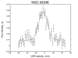
H91$\alpha$ emission was detected in six sources. The observed line profiles and Gaussian fits obtained after continuum subtraction are shown in figure 1. As we are only interested in emission around the RRL peak, non-zero baselines were used in some sources for a better fit in those regions. The flux densities per channel were obtained by integrating over the area of the UC Hii region (typically around $5^{\prime\prime}\times 5^{\prime\prime}$; see Table 2). No H91$\alpha$ emission was detected from G336.40$-$0.25, G339.88$-$1.26 or G345.01+1.79. These three regions have low continuum brightness so the expected LTE line brightness is at or below the image noise level.

Figure 1: Gaussian least-squares fits to recombination line data. Error bars indicate the average noise level in each channel. Detection for source G309.92+0.48 is marginal, and a best-fit Gaussian is shown only for illustrative purposes.

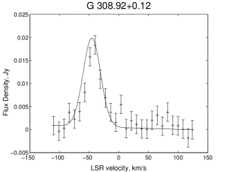
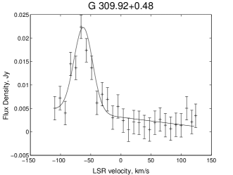
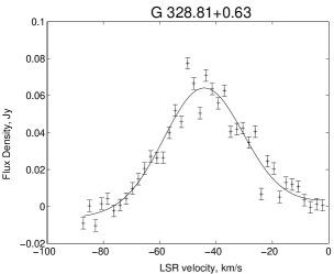
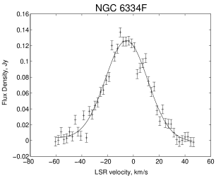
The fit parameters are given in Table 2. These were achieved using a standard non-linear least squares fitting routine, and resulted in unrealistically low error estimates for the fit parameters. In order to determine a realistic uncertainty, we made Monte-Carlo simulations, using the same routine to fit Gaussian profiles with known parameters, plus white noise of various amplitudes. Comparison of the methanol maser peak velocities from Table 1 with the H91$\alpha$ velocities from Table 2 shows approximate agreement (indicating an association between the masers and the star formation region) but sufficient difference in some cases to suggest that the masers may not be directly linked to the ionised gas. The detection is only marginal for G309.92+0.48 and thus no formal parameters were derived for this source.

Source	Vpeak	$S_{L}$	FWHM	$S_{C}$	$\Omega_{L}$	$\Omega_{C}$	$T_{C}$	$T_{e}$	source size
	(km s-1)	(mJy)	(km s-1)	(Jy)	(arcsec)	(arcsec)	(K)	(K)	(arcsec)
G 308.92+0.12	-44.4 $\pm$ 0.8	19.9 $\pm$ 1.3	34.7 $\pm$ 4.6	0.263 $\pm$ 0.0002	$7.4\times 6.1$	$7.3\times 6.8$	3900 $\pm$ 20	8200 $\pm$ 1400	$8.6\times 4$.0
G 309.92+0.48	-	-	-	0.670 $\pm$ 0.0003	$7.6\times 6.3$	$7.4\times 7.0$	-	-	$8.4\times 4.0$
G 318.95-0.20	-29.0 $\pm$ 0.4	45.1 $\pm$ 0.7	26.4 $\pm$ 1.4	0.724 $\pm$ 0.001	$8.1\times 6.4$	$8.1\times 6.8$	9630 $\pm$ 40	12600 $\pm$ 800	$7.7\times 4.0$
G 328.81+0.63	-44.5 $\pm$ 0.3	64.1 $\pm$ 1.2	33.2 $\pm$ 0.9	1.47 $\pm$ 0.0005	$8.2\times 6.1$	$8.5\times 7.0$	18370 $\pm$ 80	12900 $\pm$ 500	$6.6\times 4.0$
NGC 6334F	-5.3 $\pm$ 0.2	126.1 $\pm$ 1.6	38.8 $\pm$ 0.8	2.13 $\pm$ 0.06	$11.7\times 7.4$	$11.3\times 7.6$	18300 $\pm$ 600	10100 $\pm$ 500	$5.0\times 4.0$
NGC 6334E	-4.0 $\pm$ 0.2	57.1 $\pm$ 2.1	23.4 $\pm$ 1.3	0.417 $\pm$ 0.002	$11.7\times 7.4$	$11.3\times 7.6$	3580 $\pm$ 30	7500 $\pm$ 600	$5.0\times 4.0$

Table 2: H91$\alpha$ non-linear least squares Gaussian fits and derived parameters. Source sizes are FWZI. $S_{C}$ values are taken from ESK05. Errors for the fits are estimated from Monte Carlo simulations (see text). V_peak, $S_{L}$, and FWHM are obtained from the Gaussian fits. The electron temperature, $T_{e}$ and continuum brightness temperature, $T_{C}$ are derived as outlined in Section 3.2.1. For G 309.92+0.48 we have only a marginal detection, and hence no formal fit; as a consequence no $S_{L}$ is listed and no $T_{e}$ estimate can be made.

3.1 Arcsecond-scale emission

3.1.1 Moment maps

Image cubes for the six sources that exhibited H91$\alpha$ emission were analysed for the presence of arcsecond-scale extended emission near the UC Hii regions. Two complementary methods were employed for this analysis.

The first of these involved examining cross-cuts through the image cubes in various position-velocity planes. Positional cross-cuts were taken to run through the peak brightness position at a range of angles. Typically, the cuts were made at constant right ascension or declination or along a line joining the compact region to features of potential interest. Part a (left plots) in Figures 2 - 5 show the position-velocity plots of integrated flux density for appropriate cross-cuts in sources exhibiting significant arcsecond-scale extended emission. Position angle is calculated anticlockwise from a cut in constant declination. Position is defined as the offset from the plane passing through the point of maximum H91$\alpha$ emission. If both compact and extended components are present and physically associated, provided no strong shocks are present, their systemic velocities should be approximately equal or change smoothly between the two positions. Therefore, taking a cut along the line joining them would result in emission at the same peak velocity, but offset positionally by the distance between the two components.

Another way of determining whether any two components are likely to be associated is by plotting the first moment (a flux-weighted velocity mean across the cube) distribution across the region of H91$\alpha$ emission. This is shown in greyscale in part b (right plots) of each figure. Superimposed are the continuum contours of observations also made in the 750 D array configuration.

Figure 2: H91$\alpha$ moment maps for G318.95$-$0.20. Position-velocity plots are shown in part a (left plot). Contours are at 20 to 90% of maximum emission of 45.1 mJy beam^-1 spaced by 10%. The lowest contour of 9.0 mJy beam^-1 corresponds to $2.9\sigma$. Velocity distribution across the region is shown in grey scale in part b (right plot). Also plotted in part b are continuum contours at 10 to 90% of maximum emission of 0.724 Jy beam^-1 spaced by 10%. From the 90^∘ cross-cut (corresponding to a cut in RA), the slight western extension seems to move at a different characteristic velocity and is therefore probably not associated with other components, or is perhaps related to an outflow. A south-eastern extension is consistent with observed elongation in that direction on the continuum plot, thus the compact emission and an extension to the south-east are likely to be associated. Velocity slices suggest the amount of extended emission around this source is larger than for the others. The continuum and RRL emission are 2^′ distant from the methanol maser, suggesting that this region may be older than the other sources in our sample.

Figure 3: H91$\alpha$ moment maps for G328.81+0.63. The plots are as in Figure 2. Position-velocity contours are at 25 to 85% of maximum emission of 64.1 mJy beam^-1 spaced by 10%, with the lowest contour of 16.0 mJy beam^-1 corresponding to $4.1\sigma$. Continuum contours are at 10 to 90% of peak emission of 1.46 Jy beam^-1 spaced by 10%. Two distinct components are seen to the north and south of the compact core. Both are found to move at velocities close to those of the core, and are connected in the velocity slices. Hence the extended emission in this source is likely to be associated with the compact component. The north component coincides with the peak continuum emission observed in the continuum map, while the south extension corresponds to the cometary tail (see Figure 4 of ESK05). An additional north-west component separate from the rest of the emission also appears at approximately -35 km s^-1.

Figure 4: H91$\alpha$ moment maps for NGC 6334 E. The plots are as in Figure 2. Position-velocity contours are at 35 to 95% of maximum emission of 57.3 mJy beam^-1 spaced by 15%. The lowest contour of 20.1 mJy beam^-1 corresponds to $3.6\sigma$. Continuum contours are at 82 and 90% of peak emission. The extended and central components of the RRL emission, separated by about 20 arcseconds on the sky, are practically coincident in the 60^∘ cut shown. All cross-cuts suggest these move at a very similar velocity, and it is thus likely that they are associated. The level of background continuum emission is rather high in this source, resulting in poor image and p-v plot quality compared with other sources. High sensitivity VLA observations show NGC 6334 E to have a shell-like morphology with a weak, central compact source [2002]. This structure is not well-imaged in the ATCA observations presented here.

Figure 5: RRL H 91 $\alpha$ moment maps for NGC 6334 F. The plots are as in Figure 2. Position-velocity contours are at 20 to 90% of maximum emission of 126.1 mJy beam^-1 spaced by 10%. The lowest contour of 25.2 mJy beam^-1 corresponds to $4.5\sigma$. Continuum contours are at 10 to 90% of maximum emission of 2.13 Jy beam^-1 spaced by 10%. Arcsecond-scale emission around the core is seen to the east and south of the emission centre. The southern component appears at velocities consistent with the -5.33 km s^-1 systemic velocity of the region and represents the tail of the cometary region. The eastern component, however, peaks at velocities of about +20 km s^-1, which is significantly different from systemic region velocity and the maser velocities of approximately -10 km s^-1. Therefore, it does not appear to be associated with the compact region. This result is corroborated by the lack of significant eastern extension in the superimposed continuum contours, or the high-resolution continuum maps of ESK05. This emission is in fact known to be coincident with a massive, poorly-collimated bipolar outflow [1990, 1988, 1995b].

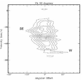
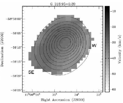
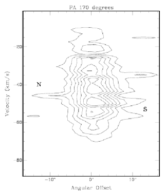
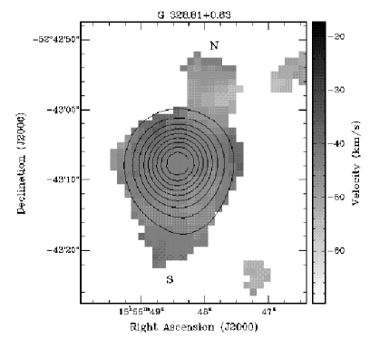
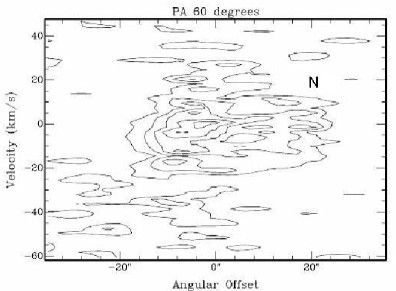
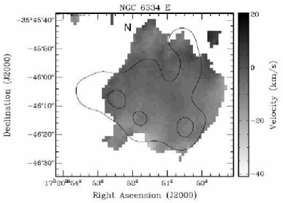
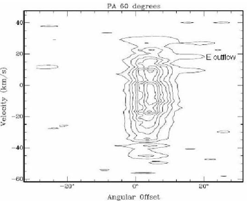
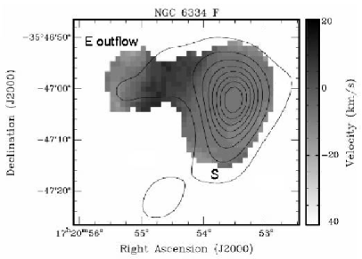
Clipping levels used in Fig. 2 - 5 were set to $2\sigma$, corresponding to 6 - 11 mJy beam^-1 depending on the source (see Table 1). Lower density gas outside the UC Hii cores is indicated in the first moment plots by presence of more emission at velocities close to the peak H91$\alpha$ velocity of the source (given in Table 2). In position-velocity plots, this corresponds to “peaks” and/or “troughs” (depending on the location of extended emission) in position at the peak RRL velocity. Evidence of such emission is seen in G 318.95$-$0.20 (Figure 2), G 328.81+0.63 (Figure 3) and NGC 6334 E (Figure 4) and F (Figure 5) components. Less arcsecond-scale emission is observed around G 308.92+0.12, and almost none at all around G 309.92+0.48. These results are consistent with the continuum observations of ESK05, and in all cases suggest association between the compact and more extended components.

Although unlikely, line-of-sight effects cannot be ruled out, as illustrated by the star-forming complex NGC 6334. The E and F components of this complex are well-known to be separate star-forming regions, separated by more than one arcminute on the sky. However, their systemic velocities are very similar, with the best fit to the E component RRL giving a peak velocity of $-4.0\pm 1.0$ km s^-1, compared with $-5.3\pm 0.6$ km s^-1 for the F component. For this reason, the two regions would have been extremely difficult to distinguish had they been superimposed along our line of sight, rather than clearly separated on the sky. This suggests that all moment analysis results should be treated with a degree of caution.

3.2 Derived Source Parameters

3.2.1 Stellar ionising flux and electron temperatures

Assuming local thermodynamic equilibrium (LTE), the electron temperature $T_{e}$ is related to the continuum and recombination line brightness temperatures $T_{C}$ and $T_{L}$, and the line Full Width at Half Maximum (FWHM) $\Delta V$ in km s^-1, by

$$\frac{T_{L}\Delta V}{T_{C}}=\frac{6983\nu^{1.1}}{T_{e}^{1.15}(1+Y^{+})}$$

where $Y^{+}$ is the fractional abundance of He⁺ by number [1981]. Assuming $Y^{+}=0.1$ and rearranging yields

$$T_{e}=\left[\frac{6348\,\nu^{1.1}T_{C}}{T_{L}\Delta V}\right]^{0.87}.$$ (1)

The continuum and recombination line brightness temperatures are related to the peak flux density $S$ (in Jy) and beam solid angle $\Omega$ via

$$T_{Bright}=\frac{S\times 10^{-26}c^{2}}{2\nu^{2}k_{B}\Omega}.$$ (2)

The continuum observations were made at $\nu_{C}=8.64$ GHz, while the H91$\alpha$ rest frequency is $\nu_{L}=8.584$ GHz. $T_{e}$ can then be determined by combining equations 1 and 2. In general, optical depth, pressure broadening, and stimulated emission must be accounted for in RRL analysis [1992]. These non-LTE effects can be significant for the H91$\alpha$ line. For expected emission measures of $\sim 10^{7}$ pc cm^-6 we use a correction factor of $\frac{T_{e}}{T_{e}^{*}}\sim 1.3$ [1983]. The values of $T_{e}$ derived above must be scaled by this factor to account for non-LTE effects. The resulting values for $T_{e}$ are shown in Table 2. They are somewhat higher than values obtained with single-dish observations [1987]. The $T_{e}$ uncertainties for most sources are quite large due to uncertainties in the H91$\alpha$ fit parameters.

We also calculate the ionising flux and stellar spectral type for each source by using the observed continuum fluxes of ESK05 and derived electron temperatures via the standard Schraml & Mezger [1969] argument. These values are given in Table 3, together with the corresponding spectral types from Panagia [1973].

3.2.2 Emission Measures

The continuum brightness temperature $T_{C}$ is related to electron temperature $T_{e}$ via the optical depth $\tau$,

$$T_{C}=T_{e}\left(1-e^{-\tau}\right)$$

Rearranging this expression, the optical depth is given by

$$\tau=-\ln\left(1-\frac{T_{C}}{T_{e}}\right)$$ (3)

From equation 2, $T_{C}$ and therefore $\tau$ can be evaluated for each source using the derived $S_{C}$ values and beam solid angles given in Table 2. From this, the peak emission measure for each source can be derived using

$$EM_{peak}=\frac{\tau}{8.235\times 10^{-2}\alpha(\nu,T_{e})T_{e}^{-1.35}\nu_{C}^{-2.1}}$$ (4)

Here, $\alpha(\nu,T_{e})$ is a correction factor of order one adopted from Mezger & Henderson [1967]. Values of $\tau$ and peak emission measure calculated for each source are shown in Table 3.

The peak emission measures thus derived were used to estimate the angular and physical sizes of the ultra-compact components of the regions. Taking ultra-compact regions to have emission measures in excess of $10^{7}$ $\mbox{pc~{}cm}^{-6}$, the cutoff emission measure fraction was determined for each source. This was defined as the lowest contour level for which emission measure exceeds $10^{7}$ $\mbox{pc~{}cm}^{-6}$, and is given by cutoff$=10^{7}/EM_{peak}$. The location of the closest contour in the 6 km continuum images of ESK05 then determined the size of the observed ultra-compact region, given in Table 3. For the purposes of comparison with our models, the sources G 308.91+0.12, G 309.92+0.48 and G 318.95$-$0.20 were considered to be spherical; while cometary sources G 328.81+0.63 and NGC 6334F were modeled with the star offset from the centre of the spherical density distribution.

Table 3: Ultra-compact component sizes derived from calculated emission measures and continuum contours of ESK05, and kinematic distances to the sources. Also given are the ionising flux for each source, derived from electron temperatures and continuum flux densities [1969] of Table 2, and the corresponding spectral type [1973]. The distances to sources are from a) Phillips et al. [1998]; b) Caswell & Haynes [1987]; and c) Ellingsen et al. [1996]. Optical depths and peak emission measures are also given where appropriate. In the case of source G 309.92$+$0.48, Caswell & Haynes [1987] electron temperature scaled for non-LTE effects is used to derive $EM_{peak}$. A scaled Caswell & Haynes [1987] electron temperature is also quoted for source G $339.88-1.26$. Continuum temperatures for sources G 328.81$+$0.63 and NGC 6334F are comparable with their electron temperatures, and we therefore adopt a lower limit of $\tau=1$ for these sources. Correction factors $\alpha$ are interpolated from Mezger & Henderson [1967] values, and range from 0.9762 to 0.9940. The cutoff fractions have been determined by comparing the derived peak emission measures with the canonical UC Hii region value of $10^{7}$ $\mbox{pc~{}cm}^{-6}$. Large uncertainties associated with calculated $T_{e}$ and $EM_{peak}$ values arise due to propagation of smaller uncertainties through calculations. Peak emission measures predicted by the model outlined in Section 4 are also given; these should be treated as order-of-magnitude estimates.

Source	Spectral	log$S_{\ast}$	Kin. Dist.	Te	$\tau$	EM${}_{peak}/10^{7}$	Cutoff	UC size	UC size	predicted EM${}_{peak}/10^{7}$
	type	(s-1)	(kpc)	(K)		($\mbox{pc~{}cm}^{-6}$)		(arcsec)	(pc)	($\mbox{pc~{}cm}^{-6}$)
G308.92$+$0.12	B 0	47.01	5.2a	$8200\pm 1400$	$0.65\pm 0.12$	$41\pm 17$	0.024	9	0.21	3.1
G309.92$+$0.48	O 7.5	48.52	5.3a	12200	$1.54\pm 0.40$	$56\pm 34$	0.018	3	0.078	5.3
G318.95$-$0.20	B 0	47.72	2.0b	$12600\pm 800$	$1.44\pm 0.10$	$56\pm 8$	0.018	13	$0.126$	2.6
G328.81$+$0.63	O 8	48.39	3.0b	$12900\pm 500$	$>1$	$41\pm 4$	0.024	6 $\times$ 11	0.087 $\times$ 0.156	4.3
G336.40$-$0.25	B 0.5	46.74	5.2a	4800	-	-	-	-	-	-
G339.88$-$1.26	B 0.5	45.99	3.0c	10000	-	-	-	-	-	-
G345.01$+$1.79	B 0	47.11	1.7c	10000	-	-	-	-	-	-
NGC 6334F	O 9	48.00	1.7c	$10100\pm 500$	$>1$	$30\pm 7$	0.034	5 $\times$ 8	0.041 $\times$ 0.066	4.4
NGC 6334E	B 0e	47.13	1.7c	$7500\pm 600$	$0.65\pm 0.07$	$13\pm 3$	0.079	-	-	3.3

4 Modeling

Detailed numerical modeling will certainly be required to address the nature of extended emission associated with UC Hii regions. In this section, we present a simple, semi-quantitative model. Franco et al. [2000a, 2000b] and Kim & Koo [2001] suggest that the ambient density structure is the primary factor determining Hii region sizes and morphologies, thereby implying the need for more realistic ambient density representation; e.g. Franco et al. [1990]. However, in the present work our focus is on the apparent association between the ultra-compact components and more diffuse arcsecond-scale extended emission [1989, 1994], and we show that this can be explained in an order of magnitude argument by a hierarchical density model.

The density structure of star-forming cores is an important modeling parameter. Numerous studies have shown that in low-mass star-forming clouds the density structure on large scales ($>1$ pc) is well-fit by power-law distributions $n\propto r^{-p}$. In high-mass star formation regions the exponent of the density power-law flattens significantly for more evolved objects, such as Hii regions [2002, 2003, 2000]. High-mass cores are less well-fit by single power-laws, and show a tendency towards clumpy substructure, possibly with the clumps embedded within overall gradients [2002, 1999]. Given the observational uncertainty regarding the magnitude of the density gradients and the scales over which they apply, we have ignored them in our modeling in favour of a simple approximation of a series of concentric spherical gas clumps.

We assume that the star forms within a hot core ($R=0.1$ pc, $T_{0}=200$ K, $n_{0}=10^{7}$ $\mbox{cm}^{-3}$), that is located within a molecular clump of radius $R=0.3$ pc, having molecular gas temperature $T_{0}=50$ K and density $n_{0}=10^{6}$ $\mbox{cm}^{-3}$, which itself lies within a molecular cloud ($R>0.3$ pc, $T_{0}=25$ K, $n_{0}=10^{5}$ $\mbox{cm}^{-3}$). The physical characteristics for the interior hot core are taken from Churchwell [2002], while those for the intermediate molecular clump are given by Cesaroni et al. [1991] and Garay & Lizano [1999], and for the exterior molecular cloud we used the parameters given by Churchwell [1999]. We note that the values we use to define hot cores and molecular clumps are indicative only and differ slightly from those used by Kim & Koo [2001].

In the simple model of Hii region evolution the radius of the expanding region is given as a function of time in terms of the initial Strömgren radius $R_{s}$ and sound speed in the ionised gas $a_{i}$ by [1980]

$$\frac{dR(t)}{dt}=a_{i}\left(\frac{R(t)}{R_{s}}\right)^{-3/4}$$ (5)

The Strömgren radius is given as

$$R_{s}=\left(\frac{3}{4\pi}\frac{S_{\ast}}{n_{0}^{2}\beta_{2}}\right)^{1/3}$$

and assuming the strong-shock limit for the expansion following the (instantaneous) formation of the Strömgren sphere, we have

$$R(t)=R_{s}\left(1+\frac{7a_{i}}{4R_{s}}t\right)^{4/7}$$

4.1 Model characteristics

4.1.1 Thermal and turbulent pressure

Given the higher thermal pressures that we now know to exist in molecular cores, Hii regions produced by O9 or later stars may still be ultra-compact when they reach pressure equilibrium with their surroundings [1995a]. The non-thermal broadening of molecular lines in high-mass star forming regions suggests that turbulence is present, with velocities of the order of 2 $\mbox{km~{}s}^{-1}$ [1996]. The resulting additional turbulent pressure $p_{turb}=n_{0}m_{H_{2}}V_{turb}^{2}$, given in terms of the molecular hydrogen mass $m_{H_{2}}$ and the turbulent velocity $V_{turb}$ in the surrounding medium, may act to restrict Hii region expansion.

Using equation 5 we can compare the relative contributions of the expanding ionisation front (I-F) and turbulence in the ambient medium to the energy balance, $\frac{E_{photo}}{E_{turb}}=\left(\frac{\frac{dR}{dt}}{V_{turb}}\right)^{2}=\frac{a_{i}^{2}}{V_{turb}^{2}}\left(\frac{R}{R_{s}}\right)^{-3/2}$

The sound speed in the ionised gas is $a_{i}=\sqrt{\frac{2k_{B}T_{e}}{m_{H}}}\sim 12.9$ km s^-1 for an electron temperature of 10 000 K. Taking an initial Strömgren radius of 0.02 pc, and UC region radius of 0.1 pc, we have $R=5R_{s}$, and $\frac{E_{photo}}{E_{turb}}\sim 3.7$. Thus, photoionisation energy nominally dominates (for $R\approx R_{s}$) but is of the same order as the turbulent energy. Turbulent velocities greater than 2 $\mbox{km~{}s}^{-1}$ could shift the balance in favour of turbulence. Moreover, as the expansion proceeds, the I-F energy dominance will die off, as $R$ grows well beyond $R_{s}$.

4.1.2 Density structure in ionised regions

Low-density extended emission on arcminute scales is observed near many UC Hii regions [1999, 2001, 2005]. By comparison, as shown in Section 3.1.1, we observe emission on arcsecond scales around the UC cores, consistent with other observations (e.g. Wood & Churchwell 1989; Kurtz et al. 1994). Inhomogeneous ambient density structure can explain this [2005]. Non-uniformity within the ionised region can also arise if the expansion velocity of the ionisation and shock fronts is much greater than the sound speed, a condition that occurs early in the Hii region expansion phase.

The expansion velocity of an Hii region slows with time, and is of the order of the sound speed when the region reaches pressure equilibrium. The diffusion timescale as the region expands into a molecular clump is of the order of the sound-crossing time $t\sim\frac{r_{clump}}{a_{i}}$. Taking $r_{clump}\sim 0.15$ pc and $a_{i}\sim 12.9$ km s^-1 as before gives $t\sim 1.5\times 10^{4}$ years. This is a significant fraction of an UC Hii region lifetime of $\sim 10^{5}$ years, and hence the ionised gas density cannot be considered uniform in all cases. This situation is further amplified by the presence of density inhomogeneities. Clearly, to model Hii regions properly, a full hydrodynamical treatment of the problem is required. Such modeling is beyond the scope of this paper, which purports only to offer a semi-quantitative plausibility argument.

4.2 Comparison with observations

Apart from NGC 6334E which happened to be in the same field of view as NGC 6334F, the nine regions presented here were selected for the presence of 6.7-GHz methanol maser emission. These masers are thought to correspond to a relatively short evolutionary phase that ends soon after the formation of the UCHii region (see ESK05). Recombination line analysis of extended emission around the majority of our sample shows that it is associated with the compact emission and thus the two must be considered together. We have compared the predictions from our model (compiled in Table 3) with the data for spherical (G 308.92+0.12, G 309.92+0.48 and G 318.95$-$0.20) and cometary (G 328.81+0.63) sources. The cometary source G 328.81+0.63 was modeled by positioning the ionising star 0.096 pc from the hot core centre. In all cases, observed region sizes agree within a factor of a few with predicted pressure equilibrium values. However, the predicted peak emission measures are consistently more than an order of magnitude less than the observed values (see Table 3). This discrepancy can be explained by the presence of significant amounts of ionised gas around the UC region on arcsecond scales, consistent with observational results of Section 3.1.1 and discussed in more detail below. The remaining sources in our sample, particularly those with complex morphologies, will require more detailed modeling than is considered here.

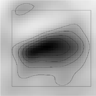
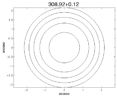
For a spherical Hii region the distance of a site line from the centre of the region is $d=rcos\theta$. The emission measure at this distance is obtained by traversing a length $2rsin\theta$. For uniform electron density, we then have $EM(d)/EM_{peak}=\left(2n_{e}^{2}rsin\theta\right)/\left(2n_{e}^{2}r\right)=sin\theta$. Thus

$$\frac{d}{r}=\sqrt{1-\left(\frac{EM(d)}{EM_{peak}}\right)^{2}}$$ (6)

The resultant theoretical contours can then be compared with observations. The ultra-compact components of sources G 308.92+0.12, G 309.92+0.48 and G 318.95$-$0.20 were largely unresolved in the 750D array results presented in ESK05, and high resolution images made with the 6 km array (also presented in ESK05) were used instead. The synthesized beam FWHM was taken as 1.2 arcseconds for all three sources. For each source, the resulting beam was then convolved with theoretical contours using the Table 3 ultra-compact region sizes. Figure 6 shows the theoretical map thus obtained, together with a high resolution image, for G 308.92+0.12. Table 4 shows the theoretical contour diameter and observed major and minor axes for each contour of each source. The final three columns give the observed/theoretical ratios for the two axes, as well as a geometric mean of the two for sources G 308.92+0.12 and G 309.92+0.48. The non-spherical nature of G 318.95$-$0.20 (much more so than the other two sources) means that we have only given the major axis values for this source.

Figure 6: Observed (left) and theoretical (right) emission measure contours for G 308.92+0.12. Both sets of contours are at 32, 47, 62, 77 and 92% of the peak emission measure. The box plotted together with the observed contours encloses the lowest (32%) theoretical contour. The predicted and observed contours are of similar physical size, with some evidence for compact core- extended arcsecond-scale emission structure.

Table 4: Theoretical and observed sizes for the three sources modeled as spherical. The observed/theoretical major and minor axis ratios are given for each contour of each source. The geometric means of the two are also given for sources G 308.92+0.12 and G 309.92+0.48. In source G 308.92+0.12, the major axis ratio is almost constant and close to one for most contours, indicating good agreement between model and observations. By comparison, the major axis ratios are less and depart significantly from unity in source G 318.95$-$0.20, consistent with extended emission observed around this source (see text). The contours for source G 309.92+0.48, although in reasonable agreement with the model, are most likely unresolved. The decrease in the observed/theoretical ratio at higher emission measure contours provides support for existence of ionised density gradients in the UC cores of all three Hii regions.

Source	EM contour	Theoretical diameter	Major	Minor	Major axis	Minor axis	Geometric
	(%)	(arcsec)	axis (arcsec)	axis (arcsec)	ratio	ratio	mean ratio
G 308.92$+$0.12	32	4.36	4.28	2.69	0.98	0.62	0.78
	47	3.80	3.61	1.89	0.95	0.47	0.67
	62	3.29	3.11	1.42	0.95	0.43	0.64
	77	2.65	2.49	0.94	0.94	0.35	0.57
	92	1.66	1.49	0.52	0.90	0.31	0.53
G 309.92$+$0.48	11	-	2.85	2.34	-	-	-
	31	-	2.05	1.72	-	-	-
	51	2.22	1.77	1.56	0.80	0.70	0.75
	71	1.67	1.31	1.14	0.78	0.68	0.73
	91	0.93	0.56	0.47	0.60	0.51	0.55
G 318.95$-$0.20	32.5	12.58	8.22	-	0.65	-	-
	52.5	11.31	6.22	-	0.55	-	-
	72.5	9.23	3.24	-	0.35	-	-
	92.5	5.08	1.25	-	0.25	-	-

In all three sources the observed/theoretical ratios decrease as we approach peak emission. Thus the observed contours are slightly denser near source core, implying the presence of density gradients in the ionised gas. For G 309.92+0.48 and especially G 308.92+0.12 the ratios are close to constant, suggesting almost uniform region density and thus that these sources are close to pressure equilibrium. This is again consistent with a lack of lower density gas observed around their UC cores. By comparison, the large spread of observed/theoretical ratios in G 318.95$-$0.20 suggests a much steeper ionised gas density gradient in this source, in keeping with observations of significant arcsecond-scale emission around its UC core. Accounting for this density gradient would raise the predicted peak emission measure and thus address the discrepancy between model and observations discussed in the previous section.

The ratios given in Table 4 are less than one for all three sources, indicating that the observed Hii region sizes are smaller than model predictions. This could be due to the Hii regions not being in pressure equilibrium with the ambient medium — an idea consistent with their young ages deduced from maser observations [1996, 1998, 2002], and also the fact that this ratio is closer to one for sources G 308.92+0.12 and G 309.92+0.48 which exhibit a more uniform density structure. G 309.92+0.48 is unresolved in the 750D array, and this is likely the main reason for the departure of observed contours from model predictions. Overestimates of stellar spectral types are another possible reason for the observed/predicted ratios being less than one, although this is less likely as radio observations typically underestimate spectral types due to dust absorption. Other confinement mechanisms may also play a role. Evidence for non-thermal broadening in the Gaussian profiles of Figure 1 lends further support to this scenario.

The above analysis is applicable to optically thin Hii regions. If we instead had a constant continuum brightness temperature (as would be expected for an optically thick source), the theoretical emission measures would be more uniform around the source core, providing an even greater discrepancy between predictions and observations.

5 Discussion

5.1 Emission Measures

The fact that some fraction of ionising photons is absorbed by dust suggests that our measured peak emission measures, which are already too high to be explained by constant density models, are underestimates. This effect can largely be ignored however, as the attenuation factor is $(1-f)^{1/3}$, where $f$ is the fraction of photons absorbed by dust [1990], which for $f\sim 0.9$ results in a decrease in the predicted peak emission measure by only a factor of two.

The large uncertainties associated with the electron temperatures we derived affect the calculated peak emission measures both directly and through the value of optical depth $\tau$ in equation 4. The logarithmic dependence of $\tau$ on $T_{e}$ will have a greater effect on the estimated peak emission measure value than directly through the power-law $T_{e}$ dependence in the denominator of equation 4. Hence the higher electron temperature estimates we have calculated compared to Caswell & Haynes [1987] suggest that, if anything, the estimated peak emission measures are likely to be underestimates. Typically, these effects largely cancel each other out, and in any case affect the derived peak emission measures by at most a factor of a few.

5.2 Lifetimes

The fundamental difference between pressure confinement and other models is that it predicts that in many cases the observed Hii regions are already in equilibrium with their surroundings, rather than still undergoing expansion. Our modeling suggests pressure equilibrium may be reached very quickly, with expansion taking place for only a fraction of the observed lifetimes of Hii regions. The lower Hii region age limits thus derived are given in Table 5. These are consistent with methanol maser emission being associated with very young massive stars.

Table 5: Lower limits on ultra-compact component ages as predicted by the hierarchical ambient density structure model. These are obtained from the time required to reach pressure equilibrium for each source.

Source	Minimum Age (years)
G 308.92$+$0.12	$2\times 10^{4}$
G 309.92$+$0.48	$6\times 10^{4}$
G 318.95$-$0.20	$3\times 10^{4}$
G 328.81$+$0.63	$5\times 10^{4}$
G 336.40$-$0.25	$6\times 10^{3}$
G 339.88$-$1.26	$2\times 10^{4}$
G 345.01$+$1.79	$5\times 10^{4}$
NGC 6334F	$4\times 10^{4}$
NGC 6334E	$8\times 10^{4}$

As discussed in section 4.1.1, turbulence may provide an additional confinement mechanism. Any non-isotropic nature of the turbulence (e.g., if it is magnetohydrodynamic; García-Segura & Franco 1996) may also contribute to the non-spherical appearance of the resulting Hii region. Further investigation of this issue is warranted.

6 Conclusions

We have detected arcsecond-scale emission around UC Hii cores. Using region parameters derived from continuum and H 91$\alpha$ recombination line data we show that although simple models of expansion in hydrostatic equilibrium reproduce the observed region sizes, their emission measures are significantly underestimated. This discrepancy can be explained by the presence of density gradients in the ionised gas, consistent with young source ages and observations of the diffuse emission.

References

- [1997] Arthur, S. J., & Lizano, S. 1997, ApJ, 484, 810
- [1990] Bachiller, R. & Cernicharo, J. 1990, A&A 239, 276
- [2002] Beuther, H., Schilke, P., Menten, K. M., Motte, F., Sridharan, T. K., Wyrowski, F. 2002, ApJ 566, 945
- [2002] Carral, P., Kurtz, S. E., Rodríguez, L. F., Menten, K., Cantó, J., & Arceo, R. 2002, AJ, 123, 2574
- [1987] Caswell, J. L., Haynes, R. F. 1987, A&A 171, 261
- [1994] Cesaroni, R., Churchwell, E., Hofner, P., Walmsley, C. M., Kurtz, S. 1994, A&A 288, 903
- [1991] Cesaroni, R., Walmsley, C. M., Kömpe, C., Churchwell, E. 1991, A&A 252, 278
- [1999] Churchwell, E. 1999, in C. J. Lada & N. D. Kylafis (eds.), in The Origins of Stars and Planetary Systems, p. 479, Kluwer, Dordrecht
- [2002] Churchwell, E. 2002, ARA&A 40, 27
- [2002] De Buizer, J. M., Walsh, A. J., Piña, R. K., Phillips, C. J., Telesco, C. M. 2002, ApJ 564, 327
- [1995a] De Pree, C. G., Rodríguez, L. F., Goss, W. M. 1995a, Rev. Mex. A&A 31, 39
- [1995b] De Pree, C. G., Rodríguez, L. F., Dickel, H. R., Goss, W. M. 1995b, ApJ 447, 220
- [1980] Dyson, J. E., Williams, D. A. 1980, Physics of the Interstellar Medium, Wiley, London
- [1995] Dyson, J. E., Williams, R. J. R., Redman, M. P. 1995, MNRAS 277, 700
- [1996] Ellingsen, S. P., Norris, R. P., McCulloch, P. M. 1996, MNRAS 279, 101
- [2003] Ellingsen, S. P., Cragg, D. M., Minier, V., Muller, E., Godfrey, P. D., 2003, MNRAS 344, 73
- [2005] Ellingsen, S. P., Shabala, S. S., Kurtz, S. E. 2005, MNRAS 357, 1003 (ESK05)
- [1999] Evans, N. J. II 1999, Annual Review of Astronomy and Astrophysics 37, 311
- [2004] Feldt, M., Puga, E., Lenzen, R., Henning, Th., Brandner, W., Stecklum, B., Langrage, A. M., Gendron, E., Rousset, G. 2004, ApJ in press
- [1997] Felli, M., Testi, L., Valdettaro, R., Wang, J.-J. 1997, ApJ 484, 375
- [1990] Franco, J., Tenorio-Tagle, G., Bodenheimer, P. 1990, ApJ 349, 126
- [2000a] Franco, J., Kurtz, S. E., García-Segura, G., Hofner, P. 2000a, Ap&SS 272, 169
- [2000b] Franco, J., Kurtz, S., Hofner, P., Testi, L., García-Segura, G., Martos, M. 2000b, ApJ 542, L143
- [1999] Garay, G. & Lizano, S. 1999, PASP 111, 1049
- [1996] García-Segura, G., Franco, J. 1996, ApJ 469, 171
- [2003] Hatchell, J., van der Tak, F. F. S. 2003, A&A 409, 589
- [1994] Hollenbach, D., Johnstone, D., Lizano, S., Shu, F. 1994, ApJ 428, 654
- [1979] Icke, V. 1979, A&A 78, 352
- [1988] Jackson, J. M., Ho, P. T. P., Haschick, A. D. 1988, ApJ 333, L73
- [2003] Keto, E. 2003, ApJ 599, 1196
- [1996] Kim, K.-T. & Koo, B.-C. 1996, Journal of the Korean Astronomical Society Supp. 29, S177
- [2001] Kim, K.-T., Koo, B.-C. 2001, ApJ 549, 979
- [2002] Kim, K.-T., Koo, B.-C. 2002, ApJ 575, 327
- [2003] Koo, B.-C., Kim, K.-T. 2003, ApJ 596, 362
- [1994] Kurtz, S. E., Churchwell, E., Wood, D. O. S. 1994, ApJS 91, 659
- [1999] Kurtz, S. E., Watson, A. M., Hofner, P., Otte, B. 1999, ApJ 514, 232
- [2005] Li, Y., MacLow M.-M., Abel, T. 1999, ApJ 610, 339 this is a radiative transfer paper, not hydro simulations!
- [1991] MacLow, M.-M., van Buren, D., Wood, D. O. S., Churchwell, E. 1991, ApJ 369, 395
- [1981] McGee, R. X., Newton, L. M. 1981, MNRAS 196, 889
- [1967] Mezger, P. G., Henderson, A. P. 1967, ApJ 147, 471
- [1973] Panagia, N. 1973, AJ 78, 929
- [1978] Panagia, N., Natta, A., Preite-Martinez, A. 1978, A&A 68, 265
- [1998] Phillips, C. J., Norris, R. P., Ellingsen, S. P., McCulloch, P. M. 1998, MNRAS 300, 1131
- [1969] Schraml, J., Mezger, P. G. 1969, ApJ 156, 269
- [1978] Spitzer, L. 1978, Physical Processes in the Interstellar Medium, Wiley, New York
- [1982] Rodríguez, L. F., Canto, J., Moran, J. M. 1982, ApJ 103, 110
- [1992] Roelfsema, P. R., Goss, W. M. 1992, A&A Rev. 4, 161
- [1983] Shaver, P. A., McGee, R. X., Newton, L. M., Danks, A. C., Pottasch, S. R. 1983, MNRAS 204, 53
- [1979] Tenorio-Tagle, G. 1979, A&A 71, 59
- [1995] Testi, L., Olmi, L., Hunt, L., Tofani, G., Felli, M., Goldsmith, P. 1995, A&A 303, 881
- [1990] van Buren, D., MacLow, M.-M., Wood, D. O. S., Churchwell, E. 1990, ApJ 353, 570
- [2000] van der Tak, F. F. S., van Dishoeck, E. F., Evans, N. J. II, Blake, G. A. 2000, ApJ 537, 283
- [1998] Walsh, A. J., Burton, M. G., Hyland, A. R., Robinson, G. 1998, MNRAS 301, 640
- [1989] Wood, D. O. S., Churchwell, E. 1989, ApJS 69, 831
- [2005] Wood, K., Haffner, L. M., Reynolds, R. J., Mathis J. S., Madsen, G. 2005, ApJ 633, 295
- [1996] Xie, T., Mundy, L. G., Vogel, S. N., Hofner, P. 1996, ApJ 473, L131