Inverse Compton scattering on solar photons,
heliospheric modulation, and neutrino astrophysics

Abstract

We study the inverse Compton scattering of solar photons by Galactic cosmic-ray electrons. We show that the $\gamma$-ray emission from this process is substantial with the maximum flux in the direction of the Sun; the angular distribution of the emission is broad. This previously-neglected foreground should be taken into account in studies of the diffuse Galactic and extragalactic $\gamma$-ray emission. Furthermore, observations by GLAST can be used to monitor the heliosphere and determine the electron spectrum as a function of position from distances as large as Saturn’s orbit to close proximity of the Sun, thus enabling unique studies of solar modulation. This paves the way for the determination of other Galactic cosmic-ray species, primarily protons, near the solar surface which will lead to accurate predictions of $\gamma$-rays from $pp$-interactions in the solar atmosphere. These albedo $\gamma$-rays will be observable by GLAST, allowing the study of deep atmospheric layers, magnetic field(s), and cosmic-ray cascade development. The latter is necessary to calculate the neutrino flux from $pp$-interactions at higher energies ($>$1 TeV). Although this flux is small, it is a “guaranteed flux” in contrast to other astrophysical sources of neutrinos, and may be detectable by km³ neutrino telescopes of the near future, such as IceCube. Since the solar core is opaque for very high-energy neutrinos, directly studying the mass distribution of the solar core may thus be possible.

1. Introduction

Interactions of Galactic cosmic-ray (CR) nuclei with the solar atmosphere have been predicted to be a source of very high energy (VHE) neutrinos (Moskalenko et al., 1991; Seckel et al., 1991; Ingelman & Thunman, 1996), and $\gamma$-rays (Seckel et al., 1991). They are the decay products of charged and neutral pions produced in interactions of CR nucleons with gas. The predictions for these albedo $\gamma$-rays give an integral flux $F_{\gamma}(>100\ {\rm MeV})\sim(0.2-0.7)\times 10^{-7}$ cm^-2 s^-1, while analysis of EGRET $\gamma$-ray telescope data has yielded only the upper limit $F_{\gamma}(>100\ {\rm MeV})=2.0\times 10^{-7}$ cm^-2 s^-1 (Thompson et al., 1997). At lower energies ($<$100 MeV) a contribution from CR electron bremsstrahlung in the solar atmosphere may exceed that from $\pi^{0}$-decay (see Fig. 4 in Strong at al., 2004a).

Cosmic-ray electrons comprise $\sim$1% of the total CR flux. However, they propagate over the heliospheric volume, which is large compared to the solar atmosphere where the albedo $\gamma$-rays are produced. The Sun emits photons that are targets for inverse Compton (IC) scattering by CR electrons. As a result the heliosphere is a diffuse source of $\gamma$-rays with a broad angular distribution. In this paper, we evaluate the importance of IC scattering within the heliosphere, and discuss the consequences of its measurement by such instruments as the upcoming Gamma Ray Large Area Space Telescope (GLAST) mission. In the following, we use units $\hbar=c=m_{e}=1$.

2. Anisotropic inverse Compton scattering in the heliosphere

The distribution of CR electrons within the heliosphere is approximately isotropic. However, the distribution of solar photons is distinctly anisotropic, with the photons propagating outward from the Sun. The expression for the IC production spectrum for an arbitrary photon angular distribution is given by eq. (8) from Moskalenko & Strong (2000):

$$\frac{dR(\gamma_{e},\epsilon_{1})}{d\epsilon_{2}}=\frac{\pi r_{e}^{2}}{\epsilon_{1}(\gamma_{e}-\epsilon_{2})^{2}}\int_{\Omega_{\nu}}d\Omega_{\nu}\,Q_{\nu}(\Omega_{\nu})$$ (1)

$$\quad\times\left[2-2\frac{\epsilon_{2}}{\gamma_{e}}\left(\frac{1}{\epsilon^{\prime}_{1}}+2\right)+\frac{\epsilon_{2}^{2}}{\gamma_{e}^{2}}\left(\frac{1}{{\epsilon^{\prime}_{1}}^{2}}+2\frac{1}{\epsilon^{\prime}_{1}}+3\right)-\frac{\epsilon_{2}^{3}}{\gamma_{e}^{3}}\right],$$

where $r_{e}$ is the classical electron radius, $\gamma_{e}$ is the electron Lorentz-factor, $\epsilon_{1}$ and $\epsilon^{\prime}_{1}$ are the energies of the background photon in the laboratory system (LS) and electron rest system, correspondingly, $\epsilon_{2}$ is the LS energy of upscattered photon, $\epsilon_{2}\leq 2\gamma_{e}\epsilon^{\prime}_{1}/(1+2\epsilon^{\prime}_{1}),\epsilon^{\prime}_{1}=\epsilon_{1}\gamma_{e}(1+\beta_{e}\cos\zeta),$ $\zeta$ is the LS angle between the momenta of the electron and incoming photon ($\zeta=0$ for head-on collisions, see Fig. 1), $\epsilon_{2\max}=4\epsilon_{1}\gamma_{e}^{2}/(1+4\epsilon_{1}\gamma_{e})$ is the maximal energy of the upscattered photons, and $Q_{\nu}(\Omega_{\nu})$ is the normalised angular distribution of target photons at a particular spatial point ($\int d\Omega_{\nu}\,Q_{\nu}=1$).

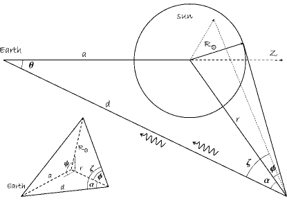
Figure 1.— Variables involved in the calculation. The large plot shows a 2-dimensional sketch; the dotted lines are a projection of the 3-dimensional angles. The inset defines the angles in 3 dimensions.

The $\gamma$-ray flux as a function of $\theta$ (see Fig. 1) can be calculated by integrating eq. (1) along the line-of-sight taking into account the distribution of electrons and solar photons:

$$\frac{dF_{\gamma}}{d\epsilon_{2}}=\frac{1}{4}\int_{L}dx\,\frac{R_{\sun}^{2}}{r^{2}}\, \int d\gamma_{e}\,\frac{dJ_{e}(r,\gamma_{e})}{d\gamma_{e}}$$

$$\times\int d\epsilon_{1}\frac{dn_{bb}(\epsilon_{1},T_{\sun})}{d\epsilon_{1}}\,\frac{dR(\gamma_{e},\epsilon_{1})}{d\epsilon_{2}},$$

where the factor $1/4$ comes from the angular distribution of photons for the case of an emitting surface (see Moskalenko & Strong 2000, eqs. [24]-[26]), $J_{e}(r,\gamma_{e})$ is the electron intensity, $r$ is the radial distance from the Sun, $R_{\sun}$ is the solar radius, and $dn_{bb}(\epsilon_{1},T_{\sun})/d\epsilon_{1}$ is a blackbody distribution at temperature $T_{\sun}$.

Close to the Sun, $Q_{\nu}(\Omega_{\nu})$ is given by

$$Q_{\nu}(r,\phi)=\frac{1}{\pi P(r)}\left(1-\frac{r^{2}}{R_{\sun}^{2}}\sin^{2}\phi\right)^{1/2},$$ (3)

$$P(r)=1-\frac{r^{2}-R_{\sun}^{2}}{2rR_{\sun}}\ln\left(\frac{r+R_{\sun}}{r-R_{\sun}}\right),$$ (4)

$$\cos\zeta=\cos\alpha\cos\phi+\sin\alpha\sin\phi\cos\psi,$$ (5)

where $\int_{0}^{2\pi}d\psi\int^{1}_{\cos\phi^{\max}}Q_{\nu}(r,\phi)\,d\cos\phi=1,$ $\sin\phi^{\max}=R_{\sun}/r$. For sufficiently large distances, this reduces to a delta function, $Q_{\nu}(\theta)=\delta(\cos\zeta-\cos\alpha)$, where $\cos\alpha=(d-a\cos\theta)/(a^{2}+d^{2}-2ad\cos\theta)^{1/2}$, $a=1$ AU, and the variables are illustrated in Fig. 1.

The IC $\gamma$-ray flux (eq. [2]) essentially falls as $1/r$ with heliocentric distance. Therefore, it is straightforward to estimate the region which contributes most to the IC emission. The inner boundary (in AU) is given by

$$r_{1}=\left\{\begin{array}[]{ll}\sin\theta,&\theta<90^{\circ},\\ 1,&\theta\geq 90^{\circ}.\end{array}\right.$$

Approximately 90% of the total $\gamma$-ray flux is produced between $r_{1}$ and $r_{2}=10r_{1}$ (Figure 2).

Figure 2.— The range of heliospheric distances probed by the IC $\gamma$-rays versus angular distance from the Sun. 90% of the predicted $\gamma$-ray flux is produced in the region between the solid and dashed lines. Dotted lines show the solar size.

The electron spectrum as a function of position in the heliosphere is obtained by adopting the force-field approximation and deriving the radial dependence of the modulation potential using a toy model. This should be sufficient, as we seek only to illustrate the effect, and are interested in electron energies above $\sim$5 GeV where the heliospheric modulation is moderate. Assuming a separability of the heliospheric diffusion coefficient $\kappa=\beta\kappa_{1}(r,t)\kappa_{2}(\gamma,t)$, the modulation potential can be obtained (Gleeson & Axford, 1968):

$$\Phi(r,t)=\int_{r}^{r_{b}(t)}dx\,\frac{V(x,t)}{3\kappa_{1}(x,t)},$$ (6)

where $t$ is the time variable, $r_{b}$ is the heliospheric boundary, and $V$ is the solar wind speed.

Fujii & McDonald (2005) have analysed the radial dependence of the mean free path, $\lambda$, during the solar minima of Cycles 20/22 and Cycle 21 using the data from the IMP 8, Voyagers 1/2, and Pioneer 10 spacecraft. For Cycles 20/22 they obtain a parameterisation $\lambda\propto r^{1.4}$ in the outer heliosphere and $\lambda\propto r^{1.1}$ in the inner heliosphere, where the break is at 10–15 AU. For Cycle 21, an $r^{1.1}$ dependence fits well for both the inner and outer heliosphere. Using these parameterisations, $\kappa_{1}\propto\lambda$, and assuming $V=const$ yields (Cycles 20/22)

$$\Phi_{1}(r)=\frac{\Phi_{0}}{1.88}\left\{\begin{array}[]{ll}r^{-0.4}-r_{b}^{-0.4},&r>r_{0},\\ 0.24+8(r^{-0.1}-r_{0}^{-0.1}),&r<r_{0},\end{array}\right.$$ (7)

where $\Phi_{0}$ is the modulation potential at 1 AU, $r_{0}=10$ AU, $r_{b}=100$ AU, and we have neglected the time dependence. For Cycle 21 we have

$$\Phi_{2}(r)=\Phi_{0}(r^{-0.1}-r_{b}^{-0.1})/(1-r_{b}^{-0.1}).$$ (8)

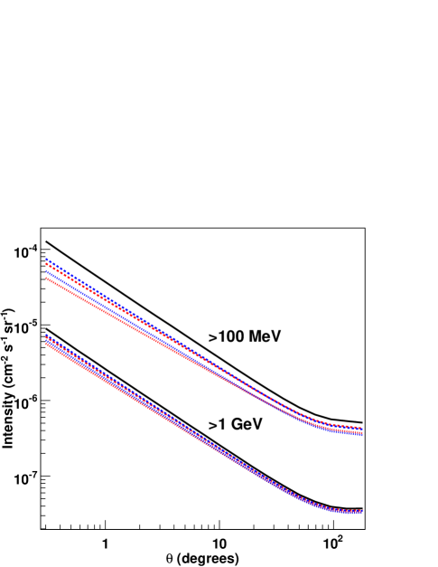
Figure 3.— Integral intensity above 100 MeV and 1 GeV. Black line: no modulation; red lines: potential $\Phi_{1}$; blue lines: potential $\Phi_{2}$. Dashed lines: $\Phi_{0}=500$ MV; dotted lines: $\Phi_{0}=1000$ MV.

3. Calculations

The local interstellar CR electron spectrum is approximated by $dJ_{e}(r_{b},\epsilon_{e})/d\epsilon_{e}=2\times 10^{5}(\epsilon_{e}+400)^{-3.22}$ cm^-2 s^-1 sr^-1 MeV^-1, where $\epsilon_{e}$ is the electron energy in MeV. This expression matches the interstellar local electron spectrum above $\sim$500 MeV as calculated by GALPROP in plain diffusion and reacceleration models (Ptuskin et al., 2006). The solar photospheric temperature is taken as $T=5770$ K (Livingston, 1999).

Figure 3 shows the integral intensity above 100 MeV and 1 GeV versus the angular distance from the Sun for no modulation, and for modulated electron spectra according to eqs. (7) and (8) with two modulation levels $\Phi_{0}=500$, 1000 MV; these correspond approximately to the solar minimum and maximum conditions, respectively. The dependency on $\Phi_{0}$ is strong and thus the emission will vary over the solar cycle while the dependency on the modulation potential parameterisation is much weaker.

The $68\%$ containment radius of the EGRET point spread function is $\sim 6^{\circ}$ at 100 MeV. For $\theta<6^{\circ}$, we calculate an integral flux $F_{\gamma}(>100\ {\rm MeV})$ $\sim 1.6\times 10^{-7}$ cm^-2 s^-1 (modulated). The sum of the IC and albedo emission (Seckel et al., 1991) over this region is consistent with the EGRET upper limit of $2\times 10^{-7}$ cm^-2 s^-1 (Thompson et al., 1997).

The differential intensities for selected angles $\theta$ are shown in Fig. 4. The parameterisations $\Phi_{1,2}$, eqs. (7) and (8), yield very similar differential $\gamma$-ray intensities; we thus show the results for $\Phi_{1}$ only. Also shown is the extragalactic $\gamma$-ray background (EGRB) obtained by Strong at al. (2004a), which includes true diffuse emission and an unresolved source component. For $\theta<5^{\circ}$, the solar IC emission is more intense than the EGRB. The latter is the major component of the diffuse $\gamma$-ray emission outside of the Galactic plane (Strong at al., 2004b). Table 1 gives the integral intensities above 10 MeV, 100 MeV, and 1 GeV averaged over the whole sky. The values for 500 MV and 1000 MV are obtained by averaging over the fluxes for $\Phi_{1}$ and $\Phi_{2}$. Above 100 MeV, the sky-averaged intensity is $\sim$5-10% of the EGRB obtained by Strong at al. (2004a).

Note that unresolved blazars are thought to be the major contributors to the EGRB (Stecker & Salamon, 1996; Kneiske & Mannheim, 2005); thousands of them will be resolved by GLAST. Therefore, the Strong at al. (2004a) EGRB flux is an upper limit for the true diffuse emission.

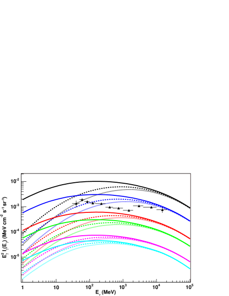
Figure 4.— Differential intensities for selected $\theta$. Line-sets (top to bottom): $0.3^{\circ}$, 1^∘, 5^∘, 10^∘, 45^∘, and 180^∘. Solid line: no modulation; dashed line: $\Phi_{0}=500$ MV; dotted line: $\Phi_{0}=1000$ MV. Data points: diffuse extragalactic $\gamma$-ray flux (Strong at al., 2004a).

4. Perspectives for GLAST

The Large Area Telescope (LAT) high-energy $\gamma$-ray detector, in preparation for launch by NASA in late 2007, will have unprecedented angular resolution, effective area, and field of view for high-energy $\gamma$-rays (McEnery et al., 2004). The LAT will scan the sky continuously and provide essentially complete sky coverage every 2 orbits (approximately 3 hours). As a consequence, the light curve for any detectable source will be well sampled. Also, the scanning motion will permit frequent evaluation of the stability of the performance of the LAT with respect to “standard candle” sources. Based on the expected sensitivity of the LAT, a source with flux $\sim$$10^{-7}$ cm^-2 s^-1 and the hardness of the solar IC emission will be detectable on a daily basis when the Sun is not close to the Galactic plane, where the diffuse emission is brightest. Sensitive variability studies of the bright core of the IC emission surrounding the Sun should be possible on weekly time scales. With exposure accumulated over several months, the Sun should be resolved as an extended source and potentially its IC, $\pi^{0}$-decay, and bremsstrahlung components separated spatially.

The extended IC emission is not isotropic, but accumulated over year timescales will be uniform in ecliptic longitude and brightest at low ecliptic latitudes. The ecliptic plane crosses the Galactic plane near the Galactic Centre, and the solar IC component may be important for investigating the nature of the reported “halo” of $\gamma$-rays about the Galactic Centre (Dixon et al., 1998).

The solar IC contribution to the overall celestial diffuse emission can be modelled directly as we have done here. Measurement of the spectrum of solar IC emission in the near Sun direction fixes the emission at all angles. This is especially true at high energies where the solar modulation in the outer heliosphere is negligible. Also, for any particular direction of the sky the Galactic and extragalactic components can be derived from the data by measuring variations in diffuse intensity with solar elongation angle.

Table 1All-sky average integral intensity

$E$	$\Phi_{0}=0$	$500$ MV	$1000$ MV
$>$10 MeV	5.9	3.7	2.5
$>$100 MeV	0.7	0.6	0.5
$>$1 GeV	0.05	0.05	0.05

Note. — Units $10^{-6}$ cm^-2 s^-1 sr^-1.

5. Discussion and Conclusion

In this paper we have studied the IC scattering of solar photons by CR electrons. We have shown that the emission is significant and broadly distributed with maximum brightness in the direction of the Sun. The whole sky is shining in $\gamma$-rays contributing to a foreground that would otherwise be ascribed to the Galactic and extragalactic diffuse emission.

The IC emission from CR electrons depends on their spectrum in the heliosphere and varies with the modulation level. Observations in different directions can be used to determine the electron spectrum at different heliocentric distances. A sensitive $\gamma$-ray telescope on orbit could monitor the heliosphere, providing information on its dynamics. Such observations also could be used to study the electron spectrum in close proximity to the Sun, unreachable for direct measurements by spacecraft. The assumed isotropy of the electron distribution everywhere in the heliosphere is an approximation. Closer to the Sun, the magnetic field and non-isotropic solar wind speed affect the CR electron spectrum and angular distribution, which in turn will produce asymmetries in the IC emission. Observations of such asymmetries may provide us with information about the magnetic field and solar wind speed at different heliolatitudes including far away from the ecliptic.

What are the immediate implications? Since solar modulation theory is well developed (e.g., Florinski et al., 2003; Ferreira & Potgieter, 2004), accurate measurement of the electron spectrum near the solar surface will open the way to derive the spectra of other Galactic CR species, primarily protons, near the Sun. The CR proton spectrum is the input to calculations of $\gamma$-rays from $pp$-interactions in the solar atmosphere. These predictions can be further tested using GLAST observations of pionic $\gamma$-rays from the Sun. In turn, this would provide information about the density profile of the solar atmosphere, magnetic field(s), and CR cascade development (Seckel et al., 1991). The higher the energy of $\gamma$-rays, the higher the energy of the ambient particles, and thus the depth of the layers tested is increased. In conjunction with other solar monitors this can bring understanding of the deep atmospheric layers, Sun spots, magnetic storms, and other solar activity.

Furthermore, understanding the solar atmosphere is necessary to calculate the neutrino flux from $pp$-interactions at higher energies ($>$1 TeV), as the CR shower development depends on the density distribution and the underlying magnetic field structure (see Seckel et al. 1991 and Ingelman & Thunman 1996 for details). Although small, the VHE neutrino flux from the Sun is a “guaranteed flux” in contrast to other astrophysical sources of neutrinos. It may be detectable by km³ neutrino telescopes of the near future, such as IceCube (e.g., Hettlage et al., 2000; Ahrens et al., 2004), on a timescale of a year or several years. Therefore, only long term periodicities associated with the solar activity could be detectable. Since the solar core is opaque for VHE neutrinos (Seckel et al., 1991; Moskalenko & Karakula, 1993; Ingelman & Thunman, 1996), observations of the neutrino flux may provide us with information about the solar mass distribution.

To summarise, we have shown that the observation of the IC emission from CR electrons in the heliosphere and its distribution on the sky will open a new chapter in astrophysics. This makes a sensitive $\gamma$-ray telescope a useful tool to monitor the heliosphere and heliospheric propagation of CR, and to study CR interactions in the solar atmosphere.

The Astrophysical Journal, 664: L143, 2007 August 1

We noticed an error in the description of the distribution of solar photons at an arbitrary distance from the Sun, equations (3) and (4). The correct expression is

$$Q_{\nu}(r,\phi)=\frac{1}{2\pi}\left[1-\left(1-\frac{R_{\odot}^{2}}{r^{2}}\right)^{1/2}\right]^{-1},$$ (1)

$$\left(1-\frac{R_{\odot}^{2}}{r^{2}}\right)^{1/2}\leq\cos\phi\leq 1,$$ (2)

i.e. $Q_{\nu}(r,\phi)$ is independent of $\phi$ within the solid angle covered by the Sun. Applying the correct angular distribution does not give results that are noticeably different from those obtained with the delta-function (pure radial) photon distribution. Indeed, it should be the case since in the energy range under consideration $\gamma_{e}\gg 1$ and the ambient photon angular distribution can be approximated by the delta-function.

We also discovered a numerical error in the code which affects the results below $\sim$1 GeV, especially in case of small $\theta$. Figures 4 and 4 show the corrected integral and differential intensities. Table 1 shows the corrected all-sky average integral intensities. The $68\%$ containment radius of the EGRET point spread function is $\sim$$6^{\circ}$ at 100 MeV. For $\theta<6^{\circ}$, the corrected integral flux is $F_{\gamma}(>100\ {\rm MeV})$ $\sim(2.0-4.3)\times 10^{-7}$ cm^-2 s^-1, where the given range corresponds to different modulation levels ($\Phi_{0}=1000-500$ MV).

Figure 3.— Integral intensity above 100 MeV and 1 GeV. Black line, no modulation; red lines, potential $\Phi_{1}$; blue lines, potential $\Phi_{2}$. Dashed lines, $\Phi_{0}=500$ MV; dotted lines, $\Phi_{0}=1000$ MV.

Figure 4.— Differential intensities for selected $\theta$. Line-sets (top to bottom): $0.3^{\circ}$, 1^∘, 5^∘, 10^∘, 45^∘, and 180^∘. Solid line: no modulation; dashed line: $\Phi_{0}=500$ MV; dotted line: $\Phi_{0}=1000$ MV. Data points: diffuse extragalactic $\gamma$-ray flux (A. W. Strong, I. V. Moskalenko, & O. Reimer [ApJ, 613,956 (2004)]).

Table 1All-sky average integral intensity

$E$		$\Phi_{0}=0$		$500$ MV		$1000$ MV
$>$10 MeV		7.1		6.5		6.0
$>$100 MeV		1.3		1.2		1.1
$>$1 GeV		0.14		0.13		0.11
Note. — Units $10^{-6}$ cm-2 s-1 sr-1.

References

- Ahrens et al. (2004) Ahrens, J., et al., 2004, New Astron. Rev., 48, 519
- Dixon et al. (1998) Dixon, D. D., et al., 1998, NewA., 3, 539
- Ferreira & Potgieter (2004) Ferreira, S. E. S., & Potgieter, M. S., 2004, ApJ, 603, 744
- Florinski et al. (2003) Florinski, V., Zank, G. P., & Pogorelov, N. V., 2003, J. Geophys. Res., 108, A6, 1228
- Fujii & McDonald (2005) Fujii, Z., & McDonald, F. B., 2005, Adv. Space Res., 35, 611
- Gleeson & Axford (1968) Gleeson, L. J., & Axford, W. I., 1968, ApJ, 154, 1011
- Hettlage et al. (2000) Hettlage, C., Mannheim, K., & Learned, J. G., 2000, APh, 13, 45
- Ingelman & Thunman (1996) Ingelman, G. & Thunman, M., 1996, Phys. Rev. D, 54, 4385
- Kneiske & Mannheim (2005) Kneiske, T. M., & Mannheim, K., 2005, in Proc. 2nd Int. Symp. on High Energy Gamma-Ray Astronomy, ed. F. A. Aharonian et al. (New York: AIP), AIP Conf. Proc., v.745, 578
- Livingston (1999) Livingston, W. C., 1999, in Allen’s Astrophysical Quantities, ed. A. N. Cox (4th ed.; New York: Springer), 339
- McEnery et al. (2004) McEnery, J. E., Moskalenko, I. V., & Ormes, J. F., 2004, in Cosmic Gamma-Ray Sources, eds. K. S. Cheng & G. E. Romero (Dordrecht: Kluwer), Astrophys. & Spa. Sci. Library, v.304, 361
- Moskalenko et al. (1991) Moskalenko, I. V., Karakula, S., & Tkaczyk, W., 1991, A&A, 248, L5
- Moskalenko & Karakula (1993) Moskalenko, I. V., & Karakula, S., 1993, J. Phys. G: Nucl. Part. Phys., 19, 1399
- Moskalenko & Strong (2000) Moskalenko, I. V., & Strong, A. W., 2000, ApJ, 528, 357
- Orlando & Strong (2006) Orlando, E., & Strong, A. W., Ap&SS, submitted (astro-ph/0607563)
- Ptuskin et al. (2006) Ptuskin, V. S., Moskalenko, I. V., Jones, F. C., Strong, A. W., & Zirakashvili, V. N., 2006, ApJ, 642, 902
- Stecker & Salamon (1996) Stecker, F. W., & Salamon, M. H., 1996, ApJ, 464, 600
- Seckel et al. (1991) Seckel, D., Stanev, T., & Gaisser, T. K., 1991, ApJ, 382, 652
- Strong at al. (2004a) Strong, A. W., Moskalenko, I. V., & Reimer, O., 2004a, ApJ, 613, 956
- Strong at al. (2004b) Strong, A. W., Moskalenko, I. V., & Reimer, O., 2004b, ApJ, 613, 962
- Thompson et al. (1997) Thompson, D. J., Bertsch, D. L., Morris, D. J., & Mukherjee, R., 1997, J. Geophys. Res. A, 120, 14735