CMB quadrupole suppression: I. Initial conditions of inflationary perturbations.

Abstract

We investigate the issue of initial conditions of curvature and tensor perturbations at the beginning of slow roll inflation and their effect on the power spectra. Renormalizability and small back reaction constrain the high $k$ behavior of the Bogoliubov coefficients that define these initial conditions. We introduce a transfer function $D(k)$ which encodes the effect of generic initial conditions on the power spectra. The constraint from renormalizability and small back reaction entails that $D(k)\lesssim\mu^{2}/k^{2}$ for large $k$, implying that observable effects from initial conditions are more prominent in the low multipoles. This behavior affects the CMB quadrupole by the observed amount $\sim 10-20\%$ when $\mu$ is of the order of the energy scale of inflation. The effects on high $l$-multipoles are suppressed by a factor $\sim 1/l^{2}$ due to the fall off of $D(k)$ for large wavevectors $k$. We show that the determination of generic initial conditions for the fluctuations is equivalent to the scattering problem by a potential $\mathcal{V}(\eta)$ localized just prior to the slow roll stage. Such potential leads to a transfer function $D(k)$ which automatically obeys the renormalizability and small backreaction constraints. We find that an attractive potential $\mathcal{V}(\eta)$ yields a suppression of the lower CMB multipoles. Both for curvature and tensor modes, the quadrupole suppression depends only on the energy scale of $\mathcal{V}(\eta)$, and on the time interval where $\mathcal{V}(\eta)$ is nonzero. A suppression of the quadrupole for curvature perturbations consistent with the data is obtained when the scale of the potential is of the order of $k^{2}_{Q}$ where $k_{Q}$ is the wavevector whose physical wavelength is the Hubble radius today.

I Introduction

Inflation is a central part of early Universe cosmology originally introduced to explain several shortcomings of the standard Big Bang cosmology guth -riottorev and at the same time it provides a mechanism for generating scalar (density) and tensor (gravitational wave) perturbations mukha -CMBgiova . A distinct aspect of inflationary perturbations is that metric perturbations are generated by quantum fluctuations of the scalar field(s) that drive inflation. After their wavelength becomes larger than the Hubble radius, these fluctuations are amplified and grow, becoming classical and decoupling from causal microphysical processes. Upon re-entering the horizon, during the matter era, these classical perturbations seed the inhomogeneities which generate structure upon gravitational collapse mukha -CMBgiova .

Most inflationary models predict fairly generic features: a gaussian, nearly scale invariant spectrum of (mostly) adiabatic scalar and tensor primordial fluctuations, making the inflationary paradigm fairly robust. The confirmation of many of the predictions of inflation by current high precision observations places inflationary cosmology on solid grounds.

The gaussian, adiabatic and nearly scale invariant spectrum of primordial fluctuations provide an excellent fit to the highly precise wealth of data provided by the Wilkinson Microwave Anisotropy Probe (WMAP)bennett -WMAP33 . Perhaps the most striking validation of inflation as a mechanism for generating superhorizon (‘acausal’) fluctuations is the anticorrelation peak in the temperature-polarization (TE) angular power spectrum at $l\sim 150$ corresponding to superhorizon scales kogut ; peiris .

The power spectra for scalar curvature and tensor (gravitational wave) quantum fluctuations generated during the inflationary stage determine the angular power spectrum of CMB anisotropies. Their initial conditions are usually chosen as Bunch-Davies conditions BD , which fix the asymptotic behavior for large negative conformal time $\eta$ to be the same as in Minkowski space time in term of positive frequencies. The Bunch-Davies states transform as irreps under the maximal symmetry group $O(4,1)$ of de Sitter space-time. (Other initial states were also considered diferen ). The requirement that the energy momentum tensor be renormalizable constrains the UV asymptotic behaviour of the Bogoliubov coefficients that encode different initial conditions motto2 .

The possibility that more precise observations of the anisotropies in the cosmic microwave background (CMB) may probe physical aspects of the initial conditions of quantum fluctuations motivated a substantial effort to study different initial conditions and their potential observational consequences otros . The remarkable high quality data and the exhaustive analysis of the three year results from WMAP WMAP31 reveal that outlaying points and wiggles near the acoustic peaks in earlier data have all but disappeared thus rendering much less statistical significance to potential observables from ‘transplanckian’ effects in the CMB otros on small angular scales.

On the other hand, while there are no statistically significant departures from the slow roll inflationary scenario at small angular scales ($l\gtrsim 100$), the third year WMAP data again confirms the surprinsingly low quadrupole $C_{2}$ WMAP31 -WMAP33 and suggests that it cannot be completely explained by galactic foreground contamination. The low value of the quadrupole has been an intriguing feature on large angular scales since first observed by COBE/DMR cobe , and confirmed by the WMAP data bennett -WMAP33 . The observation of a low quadrupole tegmark and the surprising alignment of quadrupole and octupole tegmark ; virgo sparked many different proposals for their explanation expla . More recently the robustness of these features in the low multipoles to foreground contamination has been studied tegmark2 with the suggestion abramoc2 that these may originate in extended (large scale) foregrounds perhaps generated by SZ distortions by hot electrons in the local supercluster.

The goals and main results :

In this article we address the issue of the initial conditions of the fluctuations and the effects they imprint on the primordial spectra of curvature and tensor perturbations within the effective field theory of inflation 1sN . We show that initial conditions consistent with renormalizability and small back reaction influence mainly the low CMB multipoles. In particular we find a suppression of CMB quadrupole consistent with the current observations. Furthermore, we formulate the problem of the initial conditions in terms of a potential that affects the evolution of scalar and tensor fluctuations prior to slow roll. In a companion articleII we show that this potential is a generic feature of a brief fast roll stage prior to slow roll inflation, and study its observational consequences as a suppression in the CMB quadrupole for temperature and tensor modes. We highlight that these results are derived within the context of the effective theory of inflation1sN ; clar . Namely, we provide a consistent assessment of the initial conditions at the energy scale of inflation which is the grand unification scale ($\sim 10^{16}$GeV), without the need to advocate transplanckian physics or extra assumptions as an explanation for non-BD initial conditions. As described in detail below, non-BD initial conditions can be consistently incorporated within the effective field theory valid at the inflation scale.

The goal of this article is to study the effects on the power spectra of curvature and gravitational wave perturbations of initial conditions consistent with the criteria of renormalizability of the gauge invariant energy momentum tensor and negligible back reaction. These general initial conditions are related to the Bunch-Davies initial conditions by a Bogoliubov transformation. The renormalizability criteria constrains the high $k$ behavior of the Bogoliubov coefficientsmotto2 . We show that these constraints imply that observable effects from initial conditions are more pronounced in the low multipoles, namely in the region of the angular power spectra corresponding to the Sachs-Wolfe plateau. Our main results are summarized as follows:

• We introduce a transfer function for initial conditions $D(k)$ which encodes the effect of general initial conditions on the power spectra. The constraint from renormalizability and small back reaction entail that $D(k)={\cal O}(\mu^{2}/k^{2})$ for large $k$. We show that this behavior naturally yields an observable correction to the quadrupole. This correction can account for the suppression of the quadrupole by the observed amount $\sim 10-20\%$ when the high energy tail of the initial conditions is set by the inflation scale. The corrections to higher $l$ multipoles are suppresed by a factor $\sim 1/l^{2}$ and therefore they are not observable within the present data.

• The equation for the fluctuations can be interpreted as a one dimensional Schrödinger equation with a (conformal) time dependent potential. We argue that this potential features two distinct parts: (i) the slow roll part $[(\nu^{2}-1/4)/\eta^{2}]$ which is repulsive, (like a repulsive potential barrier, $\eta$ being the conformal time, $\nu$ being $3/2$ plus slow roll parameters), and (ii) a different part $\mathcal{V}(\eta)$ with support before slow roll starts. The potential $\mathcal{V}(\eta)$ vanishes in the slow roll stage, hence it does not affect the dynamics during this stage, but its presence imprints the physical initial conditions to the fluctuations in the slow roll stage both for metric and tensor perturbations.

• We demonstrate that the problem of setting generic initial conditions in the fluctuations equation is equivalent to the scattering problem by a potential. Thus, by implementing the powerful methods of scattering theory we show that the potential $\mathcal{V}(\eta)$ yields initial conditions on the fluctuations for the beginning of slow roll whose large $k$ behavior is consistent with renormalizability. We describe the potential $\mathcal{V}(\eta)$ in a general manner and establish that an attractive potential $\mathcal{V}(\eta)$ leads to an observable suppression of the quadrupole.

• We find that the effects on the power spectrum are robust and only depend on the strength and width of the potential $\mathcal{V}(\eta)$, namely on the energy scale of $\mathcal{V}(\eta)$, which is the inflation scale, and on the time interval where $\mathcal{V}(\eta)$ is nonzero.

• Our analysis applies both to the curvature as well as the tensor fluctuations. Therefore, we predict that the initial conditions for slow roll also affect the quadrupole for B-modes.

We show in the companion article II that the potential $\mathcal{V}(\eta)$ is quite generic and originates in a stage of fast roll inflaton dynamics. This is an early stage during which the inflaton varies rapidly, slowing down to merge with the slow roll stage.

II Initial conditions and the energy momentum tensor of scalar and tensor perturbations.

The effective field theory of slow roll inflation has two main ingredients: the classical Friedmann equations in terms of a classical part of the energy momentum tensor described by a homogeneous and isotropic condensate, and a quantum part. The latter features scalar fluctuations determined by a gauge invariant combination of the scalar field (inflaton) and metric fluctuations, and a tensor component, gravitational waves. A consistency condition for this description is that the contributions from the fluctuations to the energy momentum tensor be much smaller than those from the homogeneous and isotropic condensate. The effective field theory must include renormalization counterterms so that it is insensitive to the possible ultraviolet singularities of the short wavelength fluctuations. Different initial conditions on the mode functions of the quantum fluctuations yield different values for their contribution to the energy momentum tensor. Different initial conditions on the mode functions of the quantum fluctuations yield different values for the energy momentum tensor.

Criteria for acceptable initial conditions must include the following: i) back reaction effects from the quantum fluctuations should not modify the inflationary dynamics described by the inflaton, ii) the ultraviolet counterterms that renormalize the energy momentum tensor should not depend on the particular choice of initial conditions, namely different initial conditions should not introduce new ultraviolet divergences: a single renormalization scheme, independent of initial conditions, should render the energy momentum tensor UV finite. This set of criteria imply that the ultraviolet allowed states have their large $k$ behaviour constrained up to the fourth order in $1/k$ motto2 . In ref. motto2 only the energy momentum tensor of inflaton fluctuations was considered. However, the fluctuations of the inflaton field are not gauge invariant, and in order to establish a set of criteria for UV allowed initial states in a gauge invariant manner, we must study the full gauge invariant energy momentum of scalar and tensor fluctuations.

II.1 Scalar perturbations

The gauge invariant energy momentum tensor for quadratic scalar metric fluctuations has been obtained in ref.abramo where the reader is referred to for details. Its form simplifies in longitudinal gauge, and in cosmic time it is given byabramo

$$\langle T_{00}\rangle= M^{2}_{Pl}\Bigg{[}12\;H\;\langle\psi\dot{\psi}\rangle-3\;\langle(\dot{\psi})^{2}\rangle+\frac{9}{a^{2}(t)}\;\langle(\nabla\psi)^{2}\rangle\Bigg{]}+$$ (1)

$$+\frac{1}{2}\;\langle(\dot{\phi})^{2}\rangle+\frac{\langle(\nabla\phi)^{2}\rangle}{2\,a^{2}(t)}+\frac{V^{\prime\prime}(\Phi)}{2}\;\langle\phi^{2}\rangle+2\;V^{\prime}(\Phi)\;\langle\psi\,\phi\rangle\;,$$

where $\Phi(t)$ stands for the zero mode of the inflaton field, $\phi(t,{\vec{x}})$ for the inflaton fluctuations around $\Phi(t),\;\psi(t,{\vec{x}})$ is the longitudinal gauge form of the Bardeen potential and the dots stand for derivatives with respect to cosmic time. During inflation the Newtonian potential and the Bardeen potential are the same in the longitudinal gaugemukhanov ; riotto and this property has been used in the above expression.

In longitudinal gauge, the equations of motion in cosmic time for the Fourier modes aremukhanov ; riotto

$$\ddot{\psi}_{\vec{k}}+\left(H-2\;\frac{\ddot{\Phi}}{\dot{\Phi}}\right)\dot{\psi}_{\vec{k}}+\left[2\;\left(\dot{H}-2\;H\;\frac{\ddot{\Phi}}{\dot{\Phi}}\right)+\frac{k^{2}}{a^{2}(t)}\right]{\psi}_{\vec{k}}=0\;,$$ (2)

(3)

$$\ddot{\phi}_{\vec{k}}+3\;H\;\dot{\phi}_{\vec{k}}+\left[V^{\prime\prime}[\Phi]+\frac{k^{2}}{a^{2}(t)}\right]\phi_{\vec{k}}+2\;V^{\prime}[\Phi]\;\psi_{\vec{k}}-4\;\dot{\Phi}\;\dot{\psi}_{\vec{k}}=0\;\;,$$ (4)

with the constraint equation

$$\dot{\psi}_{\vec{k}}+H\;\psi_{\vec{k}}=\frac{1}{2M^{2}_{Pl}}\;\phi_{\vec{k}}\;\dot{\Phi}\;.$$ (5)

Initial conditions on the mode functions of the quantum fluctuations correspond to an initial value problem at a fixed time hypersurface. For modes of cosmological relevance this time slice at which the initial conditions are established is such that these modes are subhorizon. Therefore, we must focus on the contribution to the energy momentum tensor from subhorizon fluctuations, and in particular in the large momentum region to assess the criteria for UV allowed states.

For subhorizon modes with wavevectors $k\gg a(t)\;H$, the solutions of the equation (2) are mukhanov

$$\psi_{\vec{k}}(t)\approx e^{\pm ik\eta}\Rightarrow\dot{\psi}_{\vec{k}}(t)\sim\frac{i\,k}{a(t)}\;{\psi}_{\vec{k}}(t)\;.$$ (6)

For $k\gg a(t)\;H$ the constraint equation (5) entails that abramo

$$\psi_{\vec{k}}(t)\approx\frac{i\,a(t)}{2\,M^{2}_{Pl}\,k}\;\dot{\Phi}\;\phi_{\vec{k}}\;.$$ (7)

In slow roll,

$$\dot{\Phi}=-\frac{V^{\prime}(\Phi)}{3\;H}\left[1+{\cal O}\left(\frac{1}{N}\right)\right]=-H\;M_{Pl}\;\sqrt{2\;\epsilon_{v}}\left[1+{\cal O}\left(\frac{1}{N}\right)\right]\;,$$ (8)

where the slow roll parameters $\epsilon_{v},\;\eta_{v}$ are of the order $1/N$ 1sN ,

$$\epsilon_{v}=\frac{M^{2}_{Pl}}{2}\;\left[\frac{V^{\prime}(\Phi)}{V(\Phi)}\right]^{2}={\cal O}\left(\frac{1}{N}\right)\quad,\quad\eta_{v}=M^{2}_{Pl}\;\frac{V^{\prime\prime}(\Phi)}{V(\Phi)}={\cal O}\left(\frac{1}{N}\right)\;,$$ (9)

and $N\sim 55$ stands for the number of efolds from horizon exit until the end of inflation. Therefore, for subhorizon modes,

$$\psi_{\vec{k}}(t)\approx-i\;\sqrt{2\;\epsilon_{v}}\;\left(\frac{H\;a(t)}{k}\right)\frac{\phi_{\vec{k}}}{2\;M_{Pl}}\;.$$ (10)

These identities, valid in the limit $k\gg a(t)\;H$ allow to obtain an estimate for the different contributions to $T_{00}$. The first line of eq.(1), namely the contribution from the Newtonian potential mode with comoving wavevector $k$ is

$$\langle T^{(\psi)}_{00}\rangle\approx 6\,\epsilon_{v}\,H^{2}\langle(\phi_{\vec{k}})^{2}\rangle\;.$$ (11)

The first three terms in the second line of eq.(1) (the quadratic contribution from the scalar field fluctuations) is

$$\langle T^{\phi}_{00}\rangle\approx\left(\frac{k}{a(t)}\right)^{2}\langle(\phi_{\vec{k}})^{2}\rangle\;,$$ (12)

and the crossed term is:

$$V^{\prime}(\Phi)\;\langle\psi_{k}\;\phi_{k}\rangle\approx\epsilon_{v}\,H^{2}\,\left(\frac{a(t)\;H}{k}\right)\langle(\phi_{\vec{k}})^{2}\rangle\;,$$ (13)

Therefore, in slow roll, $\epsilon_{v},\;\eta_{v}\ll 1$ and for subhorizon modes $k\gtrsim a(t)H$, the leading contribution to the energy momentum tensor for the scalar fluctuations is given by the contribution from the inflaton fluctuations, namely

$$\langle T_{00}\rangle\simeq\frac{1}{2}\;\langle(\dot{\phi})^{2}\rangle+\frac{\langle(\nabla\phi)^{2}\rangle}{2\,a^{2}(t)}+\frac{V^{\prime\prime}(\Phi)}{2}\;\langle\phi^{2}\rangle\,.$$ (14)

Furthermore, in terms of the slow roll parameter $\eta_{v},\;V^{\prime\prime}=3\;\eta_{v}\;H^{2}$ and for subhorizon wavevectors with $k\gg a(t)\;H$ the last term in eq.(14) is subdominant and will be neglected. Hence, the contribution to the energy momentum tensor from subhorizon fluctuations during the slow roll stage is determined by the subhorizon quantum fluctuations of the inflaton and given by

$$\langle T_{00}\rangle\simeq\frac{1}{2}\;\langle(\dot{\phi})^{2}\rangle+\frac{\langle(\nabla\phi)^{2}\rangle}{2\,a^{2}(t)}\;.$$ (15)

This analysis allows us to connect with the the results in ref.motto2 for inflaton fluctuations.

The inflaton fluctuation obeys the equation of motion

$$\ddot{\phi}_{\vec{k}}+3\;H\;\dot{\phi}_{\vec{k}}+\left[3\,H^{2}\,\eta_{v}+\frac{k^{2}}{a^{2}(t)}\right]\phi_{\vec{k}}=0\;.$$ (16)

In what follows it is convenient to pass to conformal time in terms of which, the homogeneous and isotropic FRW metric is determined by

$$ds^{2}=dt^{2}-a^{2}(t)(d\vec{x})^{2}=C^{2}(\eta)[d\eta^{2}-(d\vec{x})^{2}]\;,$$ (17)

where $t$ and $\eta$ stand for cosmic and conformal time respectively. During slow roll

$$C(\eta)=-\frac{1}{\eta H\;(1-\epsilon_{v})}\;.$$ (18)

In conformal time $\eta$ the solution of eq.(16) is given by

$$\phi_{\vec{k}}(\eta)=\frac{1}{C(\eta)}\left[\alpha_{\vec{k}}\;S_{\phi}(k,\eta)+\alpha^{\dagger}_{-\vec{k}}\;S_{\phi}^{*}(k,\eta)\right]\;,$$ (19)

where the mode functions $S_{\phi}(k,\eta)$ are solutions of

$$\left[\frac{d^{2}}{d\eta^{2}}+k^{2}+M^{2}_{\Phi}\;C^{2}(\eta)-\frac{C^{\prime\prime}(\eta)}{C(\eta)}\right]S_{\phi}(k,\eta)=0\;,$$ (20)

here,

$$M^{2}_{\Phi}=V^{\prime\prime}(\Phi)=3\;H^{2}\;\eta_{v}\;.$$ (21)

and prime stands for derivative with respect to the conformal time. Using eqs.(9) and (18) during slow roll, this equation simplifies to

$$\left[\frac{d^{2}}{d\eta^{2}}+k^{2}-\frac{\nu^{2}_{\phi}-\frac{1}{4}}{\eta^{2}}\right]S_{\phi}(k,\eta)=0\;,$$ (22)

where for inflaton fluctuations during slow-roll

$$\nu_{\phi}=\frac{3}{2}+\epsilon_{v}-\eta_{v}+{\cal O}\left(\frac{1}{N^{2}}\right)\;.$$ (23)

The operators $\alpha_{\vec{k}},\;\alpha^{\dagger}_{\vec{k}}$ in eq. (19) obey the usual canonical commutation relations.

II.2 Tensor perturbations

Tensor perturbations (gravitational waves) are gauge invariant. The expectation value of their energy momentum pseudo-tensor in a quantum state has been obtained in ref.abramo (see also ref.giova2 ) and is given by

$$\langle T^{(T)}_{00}\rangle=M^{2}_{Pl}\Bigg{\{}H\;\langle\dot{h}_{kl}h_{kl}\rangle+\frac{1}{8}\left[\langle\dot{h}_{kl}\;\dot{h}_{kl}\rangle+\frac{1}{a^{2}(t)}\langle\nabla h_{kl}\;\nabla h_{kl}\rangle\right]\Bigg{\}}\;,$$ (24)

where the dot stands for derivative with respect to cosmic time. The equations of motion for the spatial Fourier transform of the dimensionless tensor field $h$ are

$$\ddot{h}_{kl}(\vec{k})+3\;H\;\dot{h}_{kl}(\vec{k})+\frac{k^{2}}{a^{2}(t)}\;h_{kl}(\vec{k})=0\,.$$ (25)

Tensor perturbations correspond to minimally coupled massless fields with two physical polarizations. Passing to conformal time the spatial Fourier transform of the quantum fields are written as rmp ; CMBgiova

$$h_{ij}(\vec{k},\eta)=\frac{1}{C(\eta)\;M_{Pl}\;\sqrt{2}}\sum_{\lambda=\times,+}\epsilon_{ij}(\lambda,\vec{k})\left[\alpha_{\lambda,\vec{k}}\;\,S_{T}(k;\eta)+\alpha^{\dagger}_{\lambda,\vec{k}}\;\,S^{*}_{T}(k;\eta)\right]\;,$$ (26)

where $\lambda$ labels the two standard transverse and traceless polarizations $\times$ and $+$. The operators $\alpha_{\lambda,\vec{k}},\;\alpha^{\dagger}_{\lambda,\vec{k}}$ obey the usual canonical commutation relations, and $\epsilon_{ij}(\lambda,\vec{k})$ are the two independent traceless-transverse tensors constructed from the two independent polarization vectors transverse to $\hat{\bf{k}}$, chosen to be real and normalized such that $\epsilon^{i}_{j}(\lambda,\vec{k})\,\;\epsilon^{j}_{k}(\lambda^{\prime},\vec{k})=\delta^{i}_{k}\;\delta_{\lambda,\lambda^{\prime}}$.

The mode functions $S_{T}(k;\eta)$ obey the differential equation

$$S^{{}^{\prime\prime}}_{T}(k;\eta)+\left[k^{2}-\frac{C^{\prime\prime}(\eta)}{C(\eta)}\right]S_{T}(k;\eta)=0\;,$$ (27)

where in the slow roll regime,

$$\frac{C^{\prime\prime}(\eta)}{C(\eta)}=\frac{\nu^{2}_{T}-\frac{1}{4}}{\eta^{2}}~{}~{};~{}~{}\nu_{T}=\frac{3}{2}+\epsilon_{v}+{\cal O}\left(\frac{1}{N^{2}}\right)\;.$$ (28)

Thus, to leading order in slow roll the mode functions for gravitational waves obey the same equations of motion as for scalar fields but with vanishing mass, namely setting $\eta_{v}=0$.

II.3 Initial conditions

We treat both scalar and tensor perturbations on the same footing by focusing on mode functions solutions of the general equation

$$\left[\frac{d^{2}}{d\eta^{2}}+k^{2}-\frac{\nu^{2}-\frac{1}{4}}{\eta^{2}}\right]S(k,\eta)=0\;.$$ (29)

For general initial conditions we write

$$S(k;\eta)=A(k)\,g_{\nu}(k;\eta)+B(k)\,f_{\nu}(k;\eta)\;.$$ (30)

where two linearly independent solutions of eq.(29) are,

$$g_{\nu}(k;\eta) = \frac{1}{2}\;i^{\nu+\frac{1}{2}}\;\sqrt{-\pi\eta}\,H^{(1)}_{\nu}(-k\eta)\;,$$ (31)

$$f_{\nu}(k;\eta) = [g_{\nu}(k;\eta)]^{*}\;,$$ (32)

where $H^{(1)}_{\nu}(z)$ are Hankel functions. These solutions are normalized so that their Wronskian is given by

$$W[g_{\nu}(k;\eta),f_{\nu}(k;\eta)]=g^{\prime}_{\nu}(k;\eta)\;f_{\nu}(k;\eta)-g_{\nu}(k;\eta)\;f^{\prime}_{\nu}(k;\eta)=-i\;.$$ (33)

(here prime stands for derivative with respect to the conformal time). For the specific cases of scalar or tensor perturbations, the mode functions and coefficients $A(k),\;B(k)$ will feature a subscript index $\phi,\;T$, respectively.

For wavevectors deep inside the Hubble radius $|k\,\eta|\gg 1$, the mode functions for arbitrary $\nu$ have the Bunch-Davies asymptotic behavior

$$g_{\nu}(k;\eta)\buildrel\eta\to-\infty\over{=}\frac{1}{\sqrt{2\,k}}\;e^{-ik\eta}\quad,\quad f_{\nu}(k;\eta)\buildrel\eta\to-\infty\over{=}\frac{1}{\sqrt{2k}}\;e^{ik\eta}\;,$$ (34)

and for $\eta\to 0^{-}$, the mode functions behave as:

$$g_{\nu}(k;\eta)\buildrel\eta\to 0^{-}\over{=}\frac{\Gamma(\nu)}{\sqrt{2\,\pi\;k}}\;\left(\frac{2}{i\;k\;\eta}\right)^{\nu-\frac{1}{2}}\;.$$ (35)

The complex conjugate formula holds for $f_{\nu}(k;\eta)$.

In particular, in the scale invariant case $\nu=\frac{3}{2}$ which is the leading order in the slow roll expansion, the mode functions eqs.(31) simplify to

$$g_{\frac{3}{2}}(k;\eta)=\frac{e^{-ik\eta}}{\sqrt{2k}}\left[1-\frac{i}{k\eta}\right]\,.$$ (36)

The coefficients $A(k),\;{B}(k)$ for the general solution eq.(30) are determined by an initial condition on the mode functions $S(k;\eta)$ at a given initial conformal time ${\bar{\eta}}$, namely

$$B(k) = -i[g_{\nu}(k;{\bar{\eta}})\;S^{\prime}(k;{\bar{\eta}})-g^{\prime}_{\nu}(k;{\bar{\eta}})\;S(k;{\bar{\eta}})]$$ (37)

$$A(k) = -i[f^{\prime}_{\nu}(k;{\bar{\eta}})\;S(k;{\bar{\eta}})-f_{\nu}(k;{\bar{\eta}})\;S^{\prime}(k;{\bar{\eta}})]\;.$$ (38)

Canonical commutation relations for the Heisenberg fields entail that

$$|A(k)|^{2}-|B(k)|^{2}=1\;.$$ (39)

The S-vacuum state $|0\rangle_{\mathcal{S}}$ is annihilated by the operators $\alpha_{\vec{k}}$ associated with the modes $S(k;\eta)$. A different choice of the coefficients $A(k);\;B(k)$ determines different choices of vacua, the Bunch-Davies vacuum corresponds to $A(k)=1,\;B(k)=0$. An illuminating representation of these coefficients can be gleaned by computing the expectation value of the number operator in the Bunch-Davies vacuum. Consider the expansion of the fluctuation field both in terms of Bunch-Davies modes $g_{\nu}(k;\eta)$ and in terms of the general modes $S(k;\eta)$, for example for the scalar field $\phi$ (similarly for tensor fields with a subscript $T$ and corresponding normalization)

$$\phi_{\vec{k}}(\eta)=\frac{1}{C(\eta)}\left[a_{\vec{k}}\;g_{\nu_{\phi}}(k;\eta)+a^{\dagger}_{-\vec{k}}\;g^{*}_{\nu_{\phi}}(k;\eta)\right]\equiv\frac{1}{C(\eta)}\left[\alpha_{\vec{k}}\;S_{\phi}(k;\eta)+\alpha^{\dagger}_{-\vec{k}}\;S^{*}_{\phi}(k;\eta)\right]\;,$$ (40)

the creation and annihilation operators are related by a Bogoliubov transformation

$$\alpha^{\dagger}_{\vec{k}}=A_{\phi}(k)\;a^{\dagger}_{\vec{k}}-B_{\phi}(k)\;a_{-\vec{k}}\quad,\quad\alpha_{\vec{k}}={A}^{*}_{\phi}(k)\;a_{\vec{k}}-{B}^{*}_{\phi}(k)\;a^{\dagger}_{-\vec{k}}\;.$$ (41)

The Bunch-Davis vacuum $|0\rangle_{BD}$ is annihilated by $a_{\vec{k}}$, hence we find the expectation value

$${}_{BD}\langle 0|\alpha^{\dagger}_{\vec{k}}\;\alpha_{\vec{k}}|0\rangle_{BD}=|B_{\phi}(k)|^{2}=N_{\phi}(k)\;.$$ (42)

Where $N_{\phi}(k)$ is interpreted as the number of S-vacuum particles in the Bunch-Davis vacuum. In combination with the constraint eq.(39) the above result suggests the following representation for the coefficients $A(k);\;B(k)$

$$A_{\phi}(k)=\sqrt{1+N_{\phi}(k)}\;e^{i\theta_{A}(k)}~{}~{};~{}~{}B_{\phi}(k)=\sqrt{N_{\phi}(k)}\;e^{i\theta_{B}(k)}\;,$$ (43)

where $N_{\phi}(k),\;\theta_{A,{B}}(k)$ are real. The only relevant phase is the difference

$$\theta_{k}=\theta_{B}(k)-\theta_{A}(k)\;.$$ (44)

Notice that we provide the initial conditions at a given conformal time ${\bar{\eta}}$ which is obviously the same for all $k$-modes. This is the consistent manner to define the initial value problem (or Cauchy problem) for the fluctuations. This is different from what is often done in the literature when an ad-hoc dependence on $k$ is given to ${\bar{\eta}}$ otros .

II.4 The Transfer Function of Initial Conditions and its Asymptotic Behaviour

For gauge invariant scalar perturbations, the analysis leading to eq.(15) indicates that in order to study the energy momentum tensor for general initial conditions it is enough to consider the leading order in the slow roll expansion. Consistently with neglecting the contributions from the Newtonian potential as well as the term proportional to $V^{\prime\prime}[\Phi]$ for the inflaton fluctuations, we set $\nu=3/2$ in the expression for the mode functions eq.(31). This simplification results in considering the scalar field fluctuations as massless and minimally coupled to gravity.

The energy density in the vacuum state defined by the new initial conditions is

$$\rho={}_{\mathcal{S}}\langle 0|T_{00}|0\rangle_{\mathcal{S}}\,.$$ (45)

The renormalized energy density from the fluctuations of the inflaton field is found to bemotto2

$$\rho=\rho^{BD}+I_{1}+I_{2}$$ (46)

where $\rho^{BD}$ corresponds to the Bunch-Davies vacuum initial conditions $N_{k}=0$ and

$$I_{1} = \frac{1}{2\,\pi^{2}}\int_{0}^{\infty}dk\,k^{2}\,\left\{N_{\phi}(k)\,|\dot{F}(k,\eta)|^{2}+\sqrt{N_{\phi}(k)[1+N_{\phi}(k)]}\,\mathrm{Re}\left[e^{-i\theta_{k}}\left(\dot{F}(k,\eta)\right)^{2}\right]\right\}$$ (47)

$$I_{2} = \frac{1}{2\,\pi^{2}}\int_{0}^{\infty}dk\,k^{2}\,\frac{k^{2}}{a^{2}}\left\{N_{\phi}(k)\,|{F}(k,\eta)|^{2}+\sqrt{N_{\phi}(k)[1+N_{\phi}(k)]}\,\mathrm{Re}\left[e^{-i\theta_{k}}\left({F}(k,\eta)\right)^{2}\right]\right\}$$ (48)

where $F(k,\eta)$ is given in terms of the Bunch-Davis mode function eq.(36) for $\nu=3/2$ as

$$F(k,\eta)=(-H\,\eta)\;g_{\frac{3}{2}}(k,\eta)=\frac{H}{\sqrt{2\;k^{3}}}\;e^{-ik\eta}\;(i-k\;\eta)\;\,.$$ (49)

The power spectrum of the inflaton fluctuations is given by liddle ; rmp ,

$$P_{\phi}(k,t)={}_{\mathcal{S}}\langle 0||\phi_{k}(\eta)|^{2}|0\rangle_{\mathcal{S}}=P^{BD}_{\phi}(k,t)+\frac{k^{3}}{\pi^{2}}\left\{N_{\phi}(k)\;|{F}(k,\eta)|^{2}+\sqrt{N_{\phi}(k)[1+N_{\phi}(k)]}\;\mathrm{Re}\left[e^{-i\theta_{k}}\left({F}(k,\eta)\right)^{2}\right]\right\}\;,$$ (50)

where we used eq.(40) and

$$P^{BD}_{\phi}(k,t)=\frac{k^{3}}{2\pi^{2}}\;|{F}(k,\eta)|^{2}\;.$$ (51)

We find,

$$I_{1}=\frac{(H\eta)^{4}}{(2\pi)^{2}}\int_{0}^{\infty}dk\,k^{3}\left\{N_{\phi}(k)-\sqrt{N_{\phi}(k)[1+N_{\phi}(k)]}\cos[2\,k\,\eta+\theta_{k}]\right\}$$ (52)

(53)

$$I_{2}=\frac{(H^{2}\eta)^{2}}{(2\pi)^{2}}\int_{0}^{\infty}dk\,k\left\{N_{\phi}(k)\,(1+k^{2}\,\eta^{2})-\sqrt{N_{\phi}(k)[1+N_{\phi}(k)]}\left[(1-k^{2}\,\eta^{2})\cos[2\,k\,\eta+\theta_{k}]+2k\eta\sin[2\,k\,\eta+\theta_{k}]\right]\right\}\;,$$ (54)

(55)

$$P_{\phi}(k,t)=\left(\frac{H}{2\pi}\right)^{2}\left\{(1+k^{2}\,\eta^{2})[1+2\;N_{\phi}(k)]-2\;\sqrt{N_{\phi}(k)[1+N_{\phi}(k)]}\left[(1-k^{2}\,\eta^{2})\cos[2\,k\,\eta+\theta_{k}]+2\,k\,\eta\sin[2\,k\,\eta+\theta_{k}]\right]\right\}\;.$$

Evaluating the power spectrum after horizon crossing $|k\,\eta|\ll 1$, yields

$$\frac{P_{\phi}}{P^{BD}_{\phi}}\Bigg{|}_{|k\eta|\ll 1}=1+D_{\phi}(k)$$ (56)

where we have introduced the transfer function for initial conditions

$$D_{\phi}(k)=2\;|{B}_{\phi}(k)|^{2}-2\;\mathrm{Re}\left[A_{\phi}(k)B^{*}_{\phi}(k)\right]=2\;N_{\phi}(k)-2\;\sqrt{N_{\phi}(k)[1+N_{\phi}(k)]}\;\cos\theta_{k}\;.$$ (57)

The integrals $I_{1,2}$ are finite provided that asymptotically for $k\rightarrow\infty$ the occupation numbers behave as

$$N_{\phi}(k)=\mathcal{O}\left(\frac{1}{k^{4+\delta}}\right)\;,$$ (58)

with $\delta>0$. Namely, the finiteness of the energy momentum tensor constrains the asymptotic behaviour of the occupation numbers to vanish faster than $\frac{1}{k^{4}}$ for $k\to\infty$ motto2 . Of course, this asymptotic condition leaves a large freedom on the occupation numbers $N_{k}$.

We systematically impose the constraint eq.(58) which guarantees the finiteness of energy momentum tensor. This is not always the case for initial conditions considered in the literature (see otros ).

Let us establish a bound on the large momentum behavior of $N_{k}$ inserting the asymptotic behavior

$$N_{k}=N_{\mu}\left(\frac{\mu}{k}\right)^{4+\delta}\;,$$ (59)

with $0<\delta\ll 1$ in the integrals $I_{1,2}$. Namely, assuming that the integrals are dominated by the region of high momenta $k/H\gg 1$ and that the occupation number attains the largest possible values consistent with ultraviolet finiteness [eq.(58)]. We observe that $k\;|\eta|\gg 1$ in the early stages of inflation for large $k$, and that the maximum contribution from these integrals are at early time $\eta\sim-1/H$. Hence, the oscillatory terms in $I_{1},\;I_{2}$ average out and we have from eqs.(52)-(54),

$$I_{1}\sim I_{2}\sim\frac{N_{\mu}}{(2\pi)^{2}}\,\frac{\mu^{4}}{\delta}\;.$$ (60)

The contribution from the fluctuations to the energy momentum tensor does not lead to large back reaction effects affecting the inflationary dynamics provided that $I_{1},\;I_{2}\ll H^{2}\;M^{2}_{Pl}$, which yields

$${N_{\mu}}\ll 2\,\pi^{2}\;\frac{H^{2}\;M^{2}_{Pl}}{\mu^{4}}\;\delta\;.$$ (61)

Eq.(61) provides an occupation number distribution exhibiting the largest asymptotic value compatible with an UV finite energy momentum tensor. This maximal occupation number distribution falls off for $k\to\infty$ with the minimal acceptable power tail exponent $4+\delta$ with $\delta\ll 1$.

Gravitons are massless particles with two independent polarizations, therefore their energy momentum tensor is given by eq.(15) times a factor two. The first term in the energy momentum pseudotensor for gravitational waves eq.(24) features only one time derivative, which results in only one factor $k$ for large momenta, whereas the terms with two time or spatial derivatives yield $k^{2}$. Therefore, the first term is subdominant in the ultraviolet and the short wavelength contribution to the energy momentum (pseudo) tensor of gravitational waves is the same as that for a free massless scalar field, up to a factor 2 from the physical polarization states giova2 ; nuestroveff . Therefore we can directly extend the results obtained above for scalar fluctuations to the case of tensor fluctuations.

Small backreaction effects from the fluctuations is a necessary consistency condition for the validity of the inflationary scenario. In addition, the condition that different initial states should not affect the renormalization aspects of the energy momentum tensor is a consistency condition on the renormalizability of the effective field theory of inflation: the theory should be insensitive to the short distance physics for any initial conditions. These criteria lead to the following important consequences:

• If $\mu\sim M_{Pl}$ then $N_{\mu}\lesssim H^{2}/M^{2}_{Pl}\ll 1$ because $H/M_{Pl}\ll 1$ in the effective field theory expansion and the effect of initial conditions becomes negligible.

• For $\mu\sim\sqrt{H\,M_{Pl}}\sim V^{\frac{1}{4}}(\Phi)$, namely $\mu$ of the order of the scale of inflation during the slow roll stage, then $N_{\mu}\lesssim 1$. For example for $\delta\sim 0.01$ one obtains $N_{\mu}\sim 0.1$. If $\mu\ll\sqrt{H\,M_{Pl}}$, for example $\mu\sim H$, the bound eq.(61) is rather loose allowing a wide range of $N_{\mu}$ with potentially appreciable effects.

• The condition that the occupation number falls off faster than $1/k^{4}$ for large wavevector, implies that the possible effects from different initial conditions are more prominent for the smaller wavevectors, those that exited the Hubble radius the earliest. For cosmologically relevant wavevectors, these are those that crossed about $55$ e-folds before the end of inflation. Today those wavevectors correspond to the present Hubble scale, hence the low multipoles in the CMB.

We conclude that consistent with renormalizability and small back reaction there may be a substantial effect from the initial conditions when the characteristic scale $\mu\leq\sqrt{H\;M_{Pl}}$. The rapid fall-off of the occupation numbers $N_{\phi}(k)$ for subhorizon wavelengths and the back-reaction constraint eq.(61) entails that for these modes the transfer function eq.(57) for initial conditions simplifies to

$$D_{\phi}(k)\buildrel N_{\phi}(k)\ll 1\over{=}-2\;\sqrt{N_{\phi}(k)}\;\cos\theta_{k}\;,$$ (62)

and that the smaller values of $k$ yield the larger corrections from initial conditions. The result eq.(62) suggests a suppression of the power spectrum for $\cos\theta_{k}>0$. These observations will be crucial below when we study the effect of initial conditions on the multipoles of the CMB.

While this discussion focused on the fluctuations of the inflaton, they are directly applicable to the case of gauge invariant perturbations studied below.

III Effects of the Initial conditions on the Curvature Perturbations

In the previous section we focused on the backreaction effects from initial conditions beginning with the gauge invariant energy momentum tensor for scalar and tensor perturbations. Since the fluctuation modes are initialized on a fixed time hypersurface while their wavelength are well inside the Hubble radius, we established a correspondence with ref.motto2 which refer solely to the quantum fluctuations of the inflaton field. The effect of different initial conditions is encoded in the Bogoliubov coefficients, and in particular in the occupation numbers $N_{k}$ and the phases $\theta_{k}$. Ultraviolet allowed initial conditions require that $N_{k}$ diminishes faster than $1/k^{4}$ for asymptotically large momenta. Small backreaction effects require in general that $N_{k}\ll 1$.

In this section we study UV allowed initial conditions on the quantum fluctuations associated with gauge invariant variables which determine the power spectra of observables. We focus on both scalar and tensor perturbations.

III.1 Effects of Initial Conditions on the Power Spectrum

The gauge invariant curvature perturbation of the comoving hypersurfaces is given in terms of the Newtonian potential ($\psi$) and inflaton fluctuation ($\phi$) bymukhanov ; rmp

$$\mathcal{R}=-\psi-\frac{H}{\dot{\Phi}}\;\phi\;.$$ (63)

where $\dot{\Phi}$ stands for the derivative of the inflaton field $\Phi$ with respect to the cosmic time $t$.

It is convenient to introduce the gauge invariant potential mukhanov ,

$$u(\vec{x},t)=-z\;\mathcal{R}(\vec{x},t)\;,$$ (64)

where

$$z=a(t)\;\frac{\dot{\Phi}}{H}\;.$$ (65)

The spatial Fourier transform of the gauge invariant field $u(\vec{x},t)$ is expanded in terms of conformal time mode functions and creation and annihilation operators as followsmukhanov ; rmp

$$u(\vec{k},\eta)=\alpha_{\mathcal{R}}(k)\,S_{\mathcal{R}}(k;\eta)+\alpha^{\dagger}_{\mathcal{R}}(k)\,S^{*}_{\mathcal{R}}(k;\eta)$$ (66)

where the vacuum state is annihilated by the operators $\alpha_{\mathcal{R}}(k)$ and the mode functions are solutions of the equation

$$\Bigg{[}\frac{d^{2}}{d\eta^{2}}+k^{2}-\frac{1}{z}\frac{d^{2}z}{d\eta^{2}}\Bigg{]}S_{\mathcal{R}}(k;\eta)=0\,.$$ (67)

During slow roll and to leading order in slow roll variables

$$\frac{1}{z}\frac{d^{2}z}{d\eta^{2}}=\frac{2}{\eta^{2}}\Bigg{[}1+\frac{3}{2}\;(3\;\epsilon_{v}-\eta_{v})\Bigg{]}=\frac{\nu^{2}_{\mathcal{R}}-\frac{1}{4}}{\eta^{2}}\quad,\quad\nu_{\mathcal{R}}=\frac{3}{2}+3\,\epsilon_{v}-\eta_{v}+{\cal O}\left(\frac{1}{N^{2}}\right)\;.$$ (68)

The general solution of eq.(67) in the slow roll regime is given by

$$S_{\mathcal{R}}(k;\eta)=A_{\mathcal{R}}(k)\;g_{\nu_{\mathcal{R}}}(\eta)+B_{\mathcal{R}}(k)\;g^{*}_{\nu_{\mathcal{R}}}(\eta)\;,$$ (69)

where the function $g_{\nu}(\eta)$ is given by eq.(31), the Bogoliubov coefficients obey the relation (39) and can be written in terms of the occupation number of Bunch-Davis particles as in eq.(43) with the label $\mathcal{R}$ replacing $\phi$.

The power spectrum of curvature perturbations in the state with general initial conditions is given by liddle ; rmp ,

$$P_{\mathcal{R}}(k)\buildrel\eta\to 0^{-}\over{=}\frac{k^{3}}{2\;\pi^{2}}\;\Big{|}\frac{S_{\mathcal{R}}(k;\eta)}{z}\Big{|}^{2}\;.$$ (70)

From eq.(68) we see that in the slow-roll regime $z$ behaves as

$$z(\eta)=\frac{z_{0}}{(-k_{0}\;\eta)^{\nu_{R}-\frac{1}{2}}}\;,$$ (71)

where $z_{0}$ is the value of $z$ when a reference scale $k_{0}$ exits the horizon. Combining this result with the small $\eta$ limit eq.(35) we find from eqs.(70) and (71),

$$P_{\mathcal{R}}(k)=P^{BD}_{\mathcal{R}}(k)\Big{[}1+D_{\mathcal{R}}(k)\Big{]}$$ (72)

where we introduced the transfer function for the initial conditions of curvature perturbations:

$$D_{\mathcal{R}}(k) = 2\;|{B}_{\mathcal{R}}(k)|^{2}-2\;\mathrm{Re}\left[A_{\mathcal{R}}(k)\;B^{*}_{\mathcal{R}}(k)\,i^{2\nu_{R}-3}\right]=$$ (73)

$$= 2\;N_{\mathcal{R}}(k)-2\;\sqrt{N_{\mathcal{R}}(k)[1+N_{\mathcal{R}}(k)]}\;\cos\left[\theta_{k}-\pi\left(\nu_{R}-\frac{3}{2}\right)\right]$$ (75)

and

$$P^{BD}_{\mathcal{R}}(k)=\left(\frac{k}{2\,k_{0}}\right)^{3-2\;\nu_{\mathcal{R}}}\;\frac{\Gamma^{2}(\nu_{\mathcal{R}})}{\pi^{3}}\;\left(\frac{k\;H}{a(t)\;{\dot{\Phi}}}\right)_{0}^{2}\;.$$ (76)

The index $0$ refers to the time where the reference scale $k_{0}$ exits the horizon. In terms of the slow-roll parameter $\epsilon_{v}$ this expression simplifies to the usual resultliddle ; rmp

$$P^{BD}_{\mathcal{R}}(k)=\left(\frac{k}{2\,k_{0}}\right)^{n_{s}-1}\;\frac{\Gamma^{2}(\nu_{\mathcal{R}})}{\pi^{3}}\;\frac{H^{2}}{2\;\epsilon_{v}\;M_{Pl}^{2}}\equiv\mathcal{A}^{2}_{\mathcal{R}}\;\left(\frac{k}{k_{0}}\right)^{n_{s}-1}\;,$$ (77)

where the amplitude is given by

$$\mathcal{A}^{2}_{\mathcal{R}}=\frac{1}{8\,\pi^{2}\;\epsilon_{v}}\;\left(\frac{H}{M_{Pl}}\right)^{2}\left\{1+(3\;\epsilon_{v}-\eta_{v})\left[\ln 4+\psi\left(\frac{3}{2}\right)\right]+{\cal O}\left(\frac{1}{N^{2}}\right)\right\}\;,$$ (78)

$n_{s}-1=3-2\;\nu_{\mathcal{R}}=2\;\eta_{v}-6\;\epsilon_{v}$ in the slow-roll regime, $\psi(z)$ is the digamma function and $\psi\left(\frac{3}{2}\right)=-1.463510026.....\;$ . As shown above, for wavevectors of cosmological relevance, $N_{\mathcal{R}}(k)\ll 1$, hence to lowest order in slow roll ($2\;\nu_{\mathcal{R}}=3$), the transfer function for initial conditions simplifies to

$$D_{\mathcal{R}}(k)\buildrel N_{\mathcal{R}}(k)\ll 1\over{=}-2\;\sqrt{N_{\mathcal{R}}(k)}\,\cos\theta_{k}\;.$$ (79)

Therefore, for a positive $\cos\theta_{k}$, we have a negative $D_{\mathcal{R}}(k)$. That is, the initial conditions eq.(73) suppress the power in such case.

III.2 Tensor perturbations (Gravitational waves)

The quantization of tensor fluctuations for general initial conditions has been discussed in section II.2.

Following the same steps as in sec. III.1 we find the power spectrum of gravitational waves to be liddle ; rmp ,

$$P_{T}(k)\buildrel\eta\to 0^{-}\over{=}\frac{k^{3}}{2\;\pi^{2}}\;\Big{|}\frac{S_{T}(k;\eta)}{C(\eta)}\Big{|}^{2}=P^{BD}_{T}(k)\Big{[}1+D_{T}(k)\Big{]}\;,$$ (80)

where the transfer function for the initial conditions of tensor perturbations is

$$D_{T}(k)=2\;|{B}_{T}(k)|^{2}-2\;\mathrm{Re}\left[A_{T}(k)B^{*}_{T}(k)\,i^{2\nu_{T}-3}\right]=2\;N_{T}(k)-2\;\sqrt{N_{T}(k)[1+N_{T}(k)]}\,\cos\left[\theta_{k}-\pi(\nu_{T}-\frac{3}{2})\right]$$ (81)

and

$$P^{BD}_{T}(k)=\mathcal{A}^{2}_{T}\;\left(\frac{k}{k_{0}}\right)^{n_{T}}\;,$$ (82)

with

$$n_{T}=-2\;\epsilon_{v}\quad,\quad\frac{\mathcal{A}^{2}_{T}}{\mathcal{A}^{2}_{\mathcal{R}}}=r=16\;\epsilon_{v}\;.$$ (83)

The contribution from gravitational waves to the energy momentum (pseudo) tensor is gauge invariant and up to a factor of two from the polarizations is exactly of the form eq.(15) with $\phi$ replaced by $h$ nuestroveff . Thus, the constraint on the occupation number eq.(59)-(61) from the analysis of the backreaction and renormalizability translate directly to the case of gravitational waves for the occupation number $N_{T}(k)$.
This implies that corrections to the power spectrum of tensor modes from initial conditions are substantial if $\mu$, the asymptotic $k$ scale of $N_{T}(k)$, is $\mu\leq\sqrt{H\;M_{Pl}}$, that is of the order of the inflation scale [see discussion below eq.(59)].
We get from eq.(81) for $N_{T}(k)\ll 1$ and to leading order in slow roll,

$$D_{T}(k)\buildrel N_{T}(k)\ll 1\over{=}-2\;\sqrt{N_{T}(k)}\;\cos\theta_{k}\;.$$ (84)

Again, for a positive $\cos\theta_{k}$, we have a negative $D_{T}(k)$. That is, the initial conditions suppress the tensor power spectrum in such case.

IV The effect of initial conditions on the low multipoles of the CMB

We have shown above that the fast fall off of the occupation number $N(k)$ (for the corresponding perturbation) entails that initial conditions can only provide substantial corrections for perturbation modes whose wavevectors crossed out of the Hubble radius early during inflation. In turn, today these wavevectors correspond to scales of the order of the Hubble radius, namely to the low multipoles in the CMB.

In the region of the Sachs-Wolfe plateau for $l\lesssim 30$, the matter-radiation transfer function can be set equal to unity and the $C_{l}^{\prime}s$ are given bymukhanov -CMBgiova

$$C_{l}=\frac{4\pi}{9}\int_{0}^{\infty}\frac{dk}{k}\,{P}_{X}(k)\left\{j_{l}[k(\eta_{tod}-\eta_{LSS})]\right\}^{2}\;,$$ (85)

where $P_{X}$ is the power spectrum of the corresponding perturbation, $X=\mathcal{R}$ for curvature perturbations and $X=T$ for tensor perturbations, $j_{l}(x)$ are spherical Bessel functions abra and

$$\eta_{tod}-\eta_{LSS}=\frac{1}{a_{0}\;H_{0}}\,\int^{1}_{\frac{1}{1+z_{LSS}}}\frac{dx}{x\,\left[\frac{\Omega_{M}}{x}+\Omega_{\Lambda}x^{2}\right]^{\frac{1}{2}}}\;,$$ (86)

is the comoving distance between today and the last scattering surface (LSS). In the above expression we consider that the dark energy component is described by a cosmological constant. Taking $\Omega_{M}=0.28,\;\Omega_{\Lambda}=0.72,\;z_{LSS}=1100$ we find

$$\eta_{tod}-\eta_{LSS}\sim\frac{3.3}{a_{0}\;H_{0}}\;.$$ (87)

Notice that $k/[a_{0}\;H_{0}]\sim d_{H}/\lambda_{phys}(t_{0})$ is the ratio between today’s Hubble radius and the physical wavelength. The power spectra for curvature ($\mathcal{R}$) or gravitational wave (T) perturbations are of the form given by eqs.(72), (77), (80) and (82),

$${P}_{X}=\mathcal{A}^{2}_{X}\left(\frac{k}{k_{0}}\right)^{n_{s}-1}\left[1+D_{X}(k)\right]\;,$$ (88)

with $n_{s}=n_{\mathcal{R}}$ for curvature perturbations, $n_{s}=1+n_{T}$ for tensor perturbations, and $k_{0}\sim a_{0}\;H_{0}$ is a pivot scale. Then, from eq.(56), the relative change $\Delta C_{l}$ in the $C_{l}^{\prime}s$ due to the effect of generic initial conditions (generic vacua), is given by

$$C_{l}\equiv C^{BD}_{l}+\Delta C_{l}\quad,\quad\frac{\Delta C_{l}}{C_{l}}=\frac{\int^{\infty}_{0}D_{X}(\kappa\,x)~{}f_{l}(x)\,dx}{\int^{\infty}_{0}f_{l}(x)\,dx}$$ (89)

where $x=k/\kappa$ and

$$\kappa\equiv a_{0}\;H_{0}/3.3\;,$$ (90)

$D(\kappa\,x)$ is the transfer function of initial conditions for the corresponding perturbation and

$$f_{l}(x)=x^{n_{s}-2}[j_{l}(x)]^{2}\,.$$ (91)

We now focus on curvature perturbations since these are directly related to the temperature fluctuationspeiris . For $n_{s}=0.96$ WMAP31 , the functions $f_{l}(x)$ are strongly peaked at $x\sim l$. Therefore, $\frac{\Delta C_{l}}{C_{l}}$ is dominated by wavenumbers $k\sim l\;\kappa$.

Low multipoles $l$ correspond to wavelengths today of the order of the Hubble radius. These wavelengths crossed the Hubble radius about $55$ e-folds before the end of inflation. Therefore, since inflation lasted a total number of e-folds $N_{total}\gtrsim 60$, these wavevectors were subhorizon during the first few e-folds, namely during the slow roll stage $k\gg H$. As already discussed, let us take for these wavevectors the occupation number $N_{k}\ll 1$ as given by the asymptotic expression

$$N_{k}=N_{\mu}\,\left(\frac{\mu}{k}\right)^{4+\delta}~{}~{};~{}~{}0<\delta\ll 1$$ (92)

and assume that the angles $\theta_{k}$ are slowly varying functions of $k$ in the region of $k$ corresponding to today’s Hubble radius so that $\cos\theta_{k}\approx\overline{\cos\theta}$. Then, we find that the fractional change in the coefficients $C_{l}$ is given by

$$\frac{\Delta C_{l}}{C_{l}}\approx-2\;\sqrt{N_{\mu}}\;\left(\frac{3.3\;\mu}{a_{0}\;H_{0}}\right)^{2+\frac{\delta}{2}}\;\overline{\cos\theta}~{}~{}\frac{I_{l}(n_{s}-2-\frac{\delta}{2})}{I_{l}(n_{s})}$$ (93)

where

$$I_{l}(n_{s})=\frac{1}{2^{3-n_{s}}}\;\frac{\Gamma\left(3-n_{s}\right)\;\Gamma\left(\frac{2l+1-3+n_{s}+1}{2}\right)}{\Gamma^{2}\left(\frac{4-n_{s}}{2}\right)\;\Gamma\left(\frac{2l+1+3-n_{s}+1}{2}\right)}\;.$$ (94)

To obtain an estimate of the corrections, we take the values $n_{s}=1,\;\delta=0$ and find

$$\frac{\Delta C_{l}}{C_{l}}\approx-\frac{4}{3}\;\sqrt{N_{\mu}}\;\left(\frac{3.3\,\mu}{a_{0}\;H_{0}}\right)^{2}\,\frac{\overline{\cos\theta}}{(l-1)(l+2)}\;.$$ (95)

The $\sim 1/l^{2}$ behavior is a result of the $1/k^{2}$ fall off of $D(k)$, a consequence of the renormalizability condition on the occupation number. For the quadrupole, the relevant wave-vectors correspond to $x\sim 2$, namely $k_{Q}\sim a_{0}\;H_{0}$. It is convenient to write

$$k_{Q}=a_{sr}\;H_{i}=a_{0}\;H_{0}\;,$$ (96)

where $a_{sr}$ and $H_{i}$ are the scale factor and the Hubble parameter during the slow roll stage of inflation when the wavelength corresponding to today’s Hubble radius exits the horizon.

Hence, when the scale $\mu$ in the asymptotic form of the occupation number eq. (92) is of the order of the largest scale of cosmological relevance today, one has

$$\frac{\mu}{a_{0}\;H_{0}}\sim 1\;,$$ (97)

and for example with $N_{\mu}\sim 0.01$ we find that the fractional change in the quadrupole is given by:

$$\frac{\Delta C_{2}}{C_{2}}\sim-0.3\;{\overline{\cos\theta}}\;.$$ (98)

namely a suppression of the order of $\sim 10\%$ in the quadrupole provided that $\overline{\cos\theta}\sim 1$. This corresponds to $\mu$ of the order of the scale of inflation during the slow roll stage [see eq.(96)].

We emphasize that these are general arguments based on the criteria of renormalizability and small backreaction which initial conditions must fulfill.

In a companion article II we show that these initial conditions are effectively realized in inflationary dynamics. There we show that a short stage just prior to the onset of slow roll inflation and in which the inflaton field evolves fast, imprints initial conditions on the curvature perturbations corresponding to the above analysis.

V Initial Conditions as the Scattering by a potential

In the previous sections we have systematically analyzed the consequences of generic initial conditions different from Bunch-Davies, and which are UV allowed and consistent with small backreaction effects. We now provide a novel explanation of the origin of these initial conditions.

The mode equations (29) have the form of the Schrödinger equation in one dimension suggesting to consider them more generally as a potential scattering problem. The equations (20), (27 ) and (29) can be written in the form,

$$\Big{[}\frac{d^{2}}{d\eta^{2}}+k^{2}-W(\eta)\Big{]}S(k;\eta)=0$$ (99)

as a Schrödinger equation, with $\eta$ the coordinate, $k^{2}$ the energy and $W(\eta)$ a potential that depends on the coordinate $\eta$. In the cases under consideration

$$W(\eta)=\Bigg{\{}\begin{array}[]{l}z^{\prime\prime}/z~{}~{}\mathrm{for~{}curvature~{}perturbations}\\ \\ C^{\prime\prime}/C~{}~{}\mathrm{for~{}tensor~{}perturbations}\\ \end{array}\,.$$ (100)

It is convenient to explicitly separate the behavior of $W(\eta)$ during the slow roll stage by writing

$$W(\eta)=\mathcal{V}(\eta)+\frac{\nu^{2}-\frac{1}{4}}{\eta^{2}}\;,$$ (101)

where $\nu=\frac{3}{2}+{\cal O}\left(\frac{1}{N}\right)$ [see eqs.(23), (28) and (68)]. Consider the potential $\mathcal{V}(\eta)$ localized in a region of conformal time prior to the slow roll stage and which vanishes during the slow roll inflationary stage (during which cosmologically relevant modes cross out of the Hubble radius). Namely, a potential with the following properties:

$$\mathcal{V}(\eta)=\Bigg{\{}\begin{array}[]{l}\neq 0~{}\mathrm{for}~{}-\infty<\eta<{\bar{\eta}}\\ 0~{}\mathrm{for}~{}{\bar{\eta}}<\eta\\ \end{array}$$ (102)

where ${\bar{\eta}}$ is the time when slow roll starts.

With Bunch-Davies (outgoing) boundary conditions,

$$S(k;\eta)\buildrel\eta\to-\infty\over{=}e^{-ik\eta}/\sqrt{2k}\;,$$

the solution of eq.(99) for $W(\eta)$ given by eq.(101) and eq.(102) is

$$S(k;\eta)=\Bigg{\{}\begin{array}[]{l}A(k)\;g_{\nu}(k)+B(k)\;g^{*}_{\nu}(k)\;,~{}~{}\mathrm{for}~{}\eta>{\bar{\eta}}\\ \\ \frac{e^{-ik\eta}}{\sqrt{2k}}\;,~{}~{}\mathrm{for}~{}\eta\rightarrow-\infty\\ \end{array}$$ (103)

The coefficients $A(k),\;B(k)$ are obtained by matching the wave function $S(k;\eta)$ and its derivative at ${\bar{\eta}}$. $A(k)$ and $B(k)$ are simply related to the usual transmission and reflection coefficients of the scattering by a potential (see below).

We formally consider the conformal time starting at $\eta=-\infty$. However, the inflationary dynamics of the universe presumably starts at some negative value $\eta_{0}<{\bar{\eta}}$.

In this article we study the general consequences of such potential, deferring to a companion articleII a comprehensive analytic and numerical study that shows that an attractive potential of the form of eq.(102) originates naturally within the effective field theory of inflation from a brief fast roll stage just prior to slow roll.

V.1 The effect of the potential $\mathcal{V}(\eta)$ as a change in the initial conditions

In summary, the equations for the quantum fluctuations are

$$\left[\frac{d^{2}}{d\eta^{2}}+k^{2}-\frac{\nu^{2}-\frac{1}{4}}{\eta^{2}}-\mathcal{V}(\eta)\right]S(k;\eta)=0\;.$$ (104)

As discussed above the potential $\mathcal{V}(\eta)$ describes the deviation from the slow-roll dynamics during a (brief) stage prior to slow roll and is vanishingly small for $\eta>{\bar{\eta}}$, where ${\bar{\eta}}$ denotes the beginning of the slow-roll stage during which modes of cosmological relevance today exit the Hubble radius.

The retarded Green’s function $G_{k}(\eta,\eta^{\prime})$ of eq.(104) for $\mathcal{V}(\eta)\equiv 0$ obeys

$$\left[\frac{d^{2}}{d\eta^{2}}+k^{2}-\frac{\nu^{2}-\frac{1}{4}}{\eta^{2}}\right]G_{k}(\eta,\eta^{\prime})=\delta(\eta-\eta^{\prime})~{}~{};~{}~{}G_{k}(\eta,\eta^{\prime})=0~{}\mathrm{for}~{}\eta^{\prime}>\eta\quad,$$ (105)

it is given by

$$G_{k}(\eta,\eta^{\prime})=i\left[g_{\nu}(k;\eta)\;g^{*}_{\nu}(k;\eta^{\prime})-g_{\nu}(k;\eta^{\prime})\;g^{*}_{\nu}(k;\eta)\right]\Theta(\eta-\eta^{\prime})\quad,$$ (106)

where $g_{\nu}(k;\eta)$ is given by eq.(31).

The solution of the mode equation (104) can be written as an integral equation using the Green’s function eq.(106)

$$S(k;\eta)=g_{\nu}(k;\eta)+\int^{0}_{-\infty}G_{k}(\eta,\eta^{\prime})\;\mathcal{V}(\eta^{\prime})\;S(k;\eta^{\prime})\;d\eta^{\prime}\;.$$ (107)

This is the Lippmann-Schwinger equation familiar in potential scattering theory. Inserting eq.(106) into eq.(107) yields,

$$S(k;\eta)=g_{\nu}(k;\eta)+i\;g_{\nu}(k;\eta)\,\int^{\eta}_{-\infty}g^{*}_{\nu}(k;\eta^{\prime})\;\mathcal{V}(\eta^{\prime})\;S(k;\eta^{\prime})\;d\eta^{\prime}-i\;g^{*}_{\nu}(k;\eta)\,\int^{\eta}_{-\infty}g_{\nu}(k;\eta^{\prime})\;\mathcal{V}(\eta^{\prime})\;S(k;\eta^{\prime})\;d\eta^{\prime}\quad.$$ (108)

This solution has the Bunch-Davies asymptotic condition

$$S(k;\eta\rightarrow-\infty)=\frac{e^{-ik\eta}}{\sqrt{2k}}\,.$$ (109)

Since $\mathcal{V}(\eta)$ vanishes for $\eta>{\bar{\eta}}$, the mode functions $S(k;\eta)$ for $\eta>{\bar{\eta}}$ can be written as a linear combination of the mode functions $g_{\nu}(k;\eta)$ and $g^{*}_{\nu}(k;\eta)$ as follows,

$$S(k;\eta)=A(k)\;g_{\nu}(k;\eta)+B(k)\;g^{*}_{\nu}(k;\eta)\quad,\quad\eta>{\bar{\eta}}\quad,$$ (110)

where the coefficients $A(k)$ and $B(k)$ can be read from eq.(108),

$$A(k) = 1+i\int^{0}_{-\infty}g^{*}_{\nu}(k;\eta)\;\mathcal{V}(\eta)\;S(k;\eta)\;d\eta$$ (111)

$$B(k) = -i\int^{0}_{-\infty}g_{\nu}(k;\eta)\;\mathcal{V}(\eta)\;S(k;\eta)\;d\eta\;.$$ (113)

The constancy of the Wronskian $W[g_{\nu}(\eta),g^{*}_{\nu}(\eta)]=-i$ and eq.(110) imply the relation

$$|A(k)|^{2}-|B(k)|^{2}=1\quad.$$

It is clear that the action of a potential $\mathcal{V}(\eta)$ that vanishes for $\eta>{\bar{\eta}}$ is equivalent to setting initial conditions eqs.(110)-(113) on the mode functions at $\eta={\bar{\eta}}$ which subsequently evolve during the slow roll stage in which $\mathcal{V}(\eta)=0$. This is one of our main observations.

The integral equation can be solved iteratively in a perturbative expansion if the potential $\mathcal{V}(\eta)$ is small when compared to $k^{2}-(\nu^{2}-1/4)/\eta^{2}$. In such case, we can use for the coefficients $A(k),\;B(k)$ the first approximation obtained by replacing $S(k;\eta^{\prime})$ by $g_{\nu}(k;\eta^{\prime})$ in the integrals eqs.(111)-(113). This is the Born approximation, in which

$$A(k)=1+i\int^{0}_{-\infty}\mathcal{V}(\eta)\,|g_{\nu}(k;\eta)|^{2}\,d\eta\quad,\quad B(k)=-i\int^{0}_{-\infty}\mathcal{V}(\eta)\,g^{2}_{\nu}(k;\eta)\,d\eta\;.$$ (114)

These simple expressions are very illuminating. For asymptotically large $k$ eq.(34) for the mode functions can be used, and if the potential $\mathcal{V}(\eta)$ is differentiable and of compact support, an integration by parts yields

$$B(k)\buildrel k\to\infty\over{=}-\frac{1}{4\,k^{2}}\int^{0}_{-\infty}e^{-2\,i\,k\eta}\;\mathcal{V}^{\prime}(\eta)\,d\eta\;,$$ (115)

where the prime stands for derivative with respect to $\eta$. Therefore, according to the Riemann-Lebesgue lemma, $N_{k}=|B(k)|^{2}\lesssim 1/k^{4}$ for large $k$ and UV convergence in the integrals for the energy momentum tensor is guaranteed. Hence, an immediate consequence of the explanation of the initial conditions as a scattering problem with a localized potential is that these initial conditions are automatically ultraviolet allowed.

To illustrate the main aspects and highlight the main consequences, we consider now two simple potential models for $\mathcal{V}(\eta)$ localized at $\eta=\eta_{0}<{\bar{\eta}}$ and characterized by a strength $v_{0}$ and width $\Delta$. The first one has an exponential profile and the second is a square well. We solve the first one in the Born approximation while the second one is exactly solvable. These exact results agree remarkably well with the simpler Born approximation. Thus, the exactly solvable example supports the reliability of the Born approximation in the present framework.

V.2 Born approximation

As is clear from the integral equation (113) the occupation number $N(k)$ grows with the strength of the potential $\mathcal{V}(\eta)$. Moreover, as shown above, negligible backreaction requires $N(k)\ll 1$ for wavevectors of cosmological relevance. This is the regime where the Born approximation eq.(114) is reliable.

To leading order in slow roll we consider the scale invariant case, $\nu=\frac{3}{2}$ with the mode functions given by eq.(36), and model a potential localized at a time scale $\eta_{0}$ by

$$\mathcal{V}(\eta)=\frac{v_{0}}{\sqrt{\pi}}\,e^{-(\frac{\eta-\eta_{0}}{\Delta})^{2}}\;,$$ (116)

where $\overline{\eta}=\eta_{0}+\Delta$. The localization length must be $|\Delta|\ll|\eta_{0}|$ such that the potential must not influence the dynamics during slow roll, and $v_{0}$ must be small for the Born approximation to be valid. More precisely $|v_{0}\Delta|\ll k$, as seen below. Under these conditions we find,

$$A(k) = 1+i\,\frac{v_{0}\,|\Delta|}{2\;k}\left[1+\frac{1}{(k\,\eta_{0})^{2}}+\mathcal{O}\left(\Big{|}\frac{\Delta}{\eta_{0}}\Big{|}^{2}\right)\right]\;,$$ (117)

$$B(k) = -i\,\frac{v_{0}\,|\Delta|}{2\,k}\,e^{-(k\Delta)^{2}}\,e^{-2\,i\,k\,\eta_{0}}\left[1-\frac{1}{(k\,\eta_{0})^{2}}-\frac{2\,i}{(k\,\eta_{0})}+\mathcal{O}\left(\Big{|}\frac{\Delta}{\eta_{0}}\Big{|}^{2}\right)\right]\;.$$ (118)

To lowest order in $v_{0}$ the number of produced Bunch-Davies (BD) modes $N_{k}$ and the transfer function $D(k)$ are given by

$$N_{k}=\Big{(}\frac{v_{0}\,|\Delta|}{2\,k}\Big{)}^{2}\,e^{-2\,(k\,\Delta)^{2}}\,\left[1+\frac{1}{(k\,\eta_{0})^{2}}\right]^{2}\;,$$ (119)

and

$$D(k)=-\frac{v_{0}\;|\Delta|}{k}\,e^{-(k\,\Delta)^{2}}\Bigg{[}\sin\big{(}2\,k\,|\eta_{0}|\big{)}\left(1-\frac{1}{(k\,\eta_{0})^{2}}\right)+\frac{2\cos\big{(}2\,k\,|\eta_{0}|\big{)}}{k\,|\eta_{0}|}\Bigg{]}\;,$$ (120)

respectively. The particle number $N_{k}$ clearly falls off faster than any power at large $k$, thereby ensuring the ultraviolet convergence of the integrals in the energy momentum tensor.

This example reveals that a potential that is localized near a (conformal) time scale $\eta_{0}$ results in a phase difference $\sim e^{-2\,i\,k\,\eta_{0}}$ between the Bogoliubov coefficients $A(k),\,B(k)$. This is a general result that stems directly from the general expressions for these coefficients eq.(114) and that in turn results in the oscillatory component of the transfer function $D(k)$.

In the integral eq.(89) that yields the coefficients $\Delta C_{l}/C_{l}$, the transfer function $D(k)$ multiplies a function that is strongly peaked at $x\sim l$, namely, for momenta $k\sim l\;\kappa$. Therefore, if $k\;|\eta_{0}|\sim l\;\kappa\;|\eta_{0}|\gg 1$, the rapid oscillations in $D(k)$ average out in the integrand, resulting in a vanishing contribution to the $\Delta C_{l}/C_{l}^{\prime}s$. Hence, there are significant contributions to $\Delta C_{l}/C_{l}$ only when $l\;\kappa\;|\eta_{0}|\sim 1$. For the quadrupole this corresponds to, $[a_{0}\ H_{0}\,|\eta_{0}|]\sim 1$.

The potential ${\mathcal{V}}(\eta)$ acts prior to the slow roll stage during which cosmologically relevant modes cross the Hubble radius. For the corrections to the low multipoles be substantial, the condition for wavevectors corresponding to the Hubble radius today is $k\sim a_{0}\,H_{0}$ and $k\,|\eta_{0}|\sim 1$. The conclusion is that modifications to the low multipoles arise from a potential $\mathcal{V}(\eta)$ localized just prior to horizon crossing of the modes whose wavelengths correspond to the Hubble radius today. It is also clear that the corrections for higher wavevectors are strongly suppressed because of the rapid fall off of $B(k)$.

Furthermore, in the Born approximation the sign of the correction $\Delta C_{l}/C_{l}$ is determined by the sign of the potential. In the example given above with the potential eq.(116), it is given by the sign of $v_{0}$, negative (positive) $v_{0}$ corresponding to an attractive (repulsive) potential. Fig. 1 shows the quadrupole correction $\Delta C_{2}/C_{2}$ determined by the transfer function eq.(120) for an attractive potential ($v_{0}=-|v_{0}|$) clearly revealing a suppression for $\kappa|\eta_{0}|\sim 1$.

Figure 1: The quadrupole correction $(\Delta C_{2}/C_{2})/|v_{0}\eta_{0}\Delta|$ vs, $\kappa|\eta_{0}|$ in the Born approximation for an attractive potential of the form (116), for $|\Delta/\eta_{0}|=0.01,\;0.05,\;0.1$. Here, $\kappa=\frac{a_{0}H_{0}}{3.3}$. It clearly reveals a suppression for $\kappa\eta_{0}\sim 1$, that is for the modes whose wavelengths correspond to the Hubble radius today

The corrections for the higher multipoles are substantially smaller, vanishing very rapidly for $l\geq 3$ as shown in Fig. 2 for the attractive potential.

Figure 2: The corrections $(\Delta C_{l}/C_{l})/|v_{0}\;\eta_{0}\;\Delta|$ vs. $l$ in the Born approximation for an attractive potential of the form (116), for $\kappa\;|\eta_{0}|=1;\;|\Delta/\eta_{0}|=0.01$. The corrections for the higher multipoles are substantially smaller than the quadrupole correction, vanishing very rapidly for $l\geq 3$

V.3 Exactly solvable Potential

The Born approximation is the first order in perturbation theory and is valid in the regime $k\gg|v_{0}|$. A simple and exactly solvable example is the square well potential

$$\mathcal{V}(\eta)=\left\{\begin{array}[]{cc}-|v_{0}|&\mathrm{for}~{}~{}\eta_{1}\leq\eta\leq\eta_{2}\;,\\ 0&\textrm{otherwise}\;,\\ \end{array}\right.\;,$$ (121)

where $\eta_{1}\equiv\eta_{0}-\frac{\Delta}{2}$ and $\eta_{2}\equiv\eta_{0}+\frac{\Delta}{2}$, $\Delta>0$ is the width of the potential well and $-|v_{0}|$ its depth. The case of a potential barrier is obtained by the replacement $|v_{0}|\rightarrow-|v_{0}|$.

We compute the mode functions by matching the functions and derivatives as in the familiar case of the step-potential in the one-dimensional Schroedinger equation, and again to lowest order in slow roll we consider the scale invariant case $\nu=3/2$. The wave function is given by

$$S(k,\eta)=\left\{\begin{array}[]{cc}g(k\eta)&\;,~{}~{}\eta<\eta_{1}\\ \\ E(k)\,g(q\eta)+Q(k)\,g^{*}(q\eta)&\;,~{}~{}\eta_{1}\leq\eta\leq\eta_{2}\;,\\ \\ A(k)\,g(k\eta)+B(k)\,g^{*}(k\eta)&\;,~{}~{}\eta_{2}<\eta<0\;,\\ \end{array}\right.$$ (122)

where

$$g(k\eta)=e^{-i\,k\,\eta}\Big{[}1-\frac{i}{k\,\eta}\Big{]}~{}~{};~{}~{}q=\sqrt{k^{2}+|v_{0}|}\;.$$ (123)

Matching functions and derivatives at $\eta=\eta_{1}$ and $\eta=\eta_{2}$, we find

$$A(k)=\frac{e^{i\,k\,\Delta}}{4\,k\,q}\Bigg{\{}e^{-i\,q\,\Delta}(k+q)^{2}\Big{[}1+i\frac{k-q}{k\,q\,\eta_{1}}\Big{]}\Big{[}1-i\frac{k-q}{k\,q\ \,\eta_{2}}\Big{]}-e^{i\,q\,\Delta}(k-q)^{2}\Big{[}1-i\frac{k+q}{k\,q\,\eta_{1}}\Big{]}\Big{[}1+i\frac{k+q}{k\,q\,\eta_{2}}\Big{]}\Bigg{\}}\;,$$ (124)

(125)

$$B(k)=-|v_{0}|\,\frac{e^{-2ik\eta_{0}}}{4kq}\Bigg{\{}e^{-iq\Delta}\Big{[}1+i\frac{k-q}{k\,q\,\eta_{1}}\Big{]}\Big{[}1-i\frac{k+q}{k\,q\,\eta_{2}}\Big{]}-e^{i\,q\,\Delta}\Big{[}1-i\frac{k+q}{k\,q\,\eta_{1}}\Big{]}\Big{[}1+i\frac{k-q}{k\,q\,\eta_{2}}\Big{]}\Bigg{\}}\;.$$ (126)

It is straightforward to check the unitarity condition $|A(k)|^{2}-|B(k)|^{2}=1$. We consider an arbitrary depth $|v_{0}|$ to include non-perturbative aspects, but focus on the case of a narrow well for which

$$\Big{|}\frac{\Delta}{\eta_{0}}\Big{|}\ll 1\;.$$ (127)

The number of particles created by the pre-slow roll stage is

$$N_{k}=|B(k)|^{2}=\frac{(v_{0}\;\eta_{0}^{2})^{2}}{4(k\;\eta_{0})^{2}}\Big{|}\frac{\Delta}{\eta_{0}}\Big{|}^{2}\Bigg{\{}\Bigg{[}\frac{\sin q\,\Delta}{q\;\Delta}\left(1-\frac{|v_{0}|}{(k\;q\;\eta_{0})^{2}}\right)-\frac{\cos q\,\Delta}{(q\;\eta_{0})^{2}}\Bigg{]}^{2}+\Bigg{[}\frac{2}{k\;\eta_{0}}\frac{\sin q\,\Delta}{q\;\Delta}\Bigg{]}^{2}\Bigg{\}}\;.$$ (128)

For arbitrary strength of the potential $v_{0}$, a small number of produced particles requires a narrow width (127).

For $k\gg|v_{0}|$ the number of particles is

$$N_{k}\buildrel k\to\infty\over{=}\frac{v_{0}^{2}}{8\;k^{4}}\quad.$$ (129)

Moreover, a continuous and differentiable potential $\mathcal{V}(\eta)$ with smooth edges will yield a $N_{k}$ vanishing faster than $1/k^{4}$ for large $k$ since the Fourier transform of a continuous and differentiable function of compact support falls off exponentially at large $k$. Therefore, the asymptotic behavior for a general continuous potential with a typical scale $v_{0}$ is $N_{k}<v^{2}_{0}/k^{4}$ and the ultraviolet finiteness of the energy momentum tensor is guaranteed motto2 .

To leading order in the ‘narrow width’ approximation the transfer function is

$$D(k)=\frac{|v_{0}|\,\eta_{0}^{2}}{k\,|\eta_{0}|}\,\Big{|}\frac{\Delta}{\eta_{0}}\Big{|}\Bigg{\{}\sin(2\,k\,|\eta_{0}|)\Big{[}\frac{\sin q\,\Delta}{q\,\Delta}\left(1-\frac{|v_{0}|\,\eta_{0}^{2}}{(k\,q\,\eta_{0}^{2})^{2}}\right)-\frac{\cos q\,\Delta}{(q\,\eta_{0})^{2}}\Big{]}+2\;\frac{\cos 2\,k\,\eta_{0}}{k\,|\eta_{0}|}\,\frac{\sin q\,\Delta}{q\,\Delta}\Bigg{\}}\,,$$ (130)

where we have written the transfer function explicitly in terms of the relevant dimensionless combinations of parameters $v_{0},\;\Delta$ and $\eta_{0}$.

We have performed an exhaustive numerical study of the corrections to the $C_{l}^{\prime}s$ in a wide range of the dimensionless parameters $\kappa\;|\eta_{0}|,\;|v_{0}|\;\eta_{0}^{2}$ and $|\Delta/\eta_{0}|$ where $\kappa$ is defined in eq.(90), with the conclusion that for an attractive potential there is a substantial suppression of the quadrupole for $\kappa\;|\eta_{0}|\sim 1$ and that the corrections for higher multipoles are negligibly small and observationally irrelevant since these fall off as $1/l^{2}$, hence much smaller than the irreducible cosmic variance.

Fig. 3 displays the changes in the quadrupole for various representative values of $|v_{0}|\;\eta_{0}^{2}$ for the cases $|\Delta/\eta_{0}|=0.01,\;0.1$ respectively. It is clear from these figures that there is a substantial suppression of the quadrupole if the potential is localized at a time scale $|\eta_{0}|\sim 1/[a_{0}\;H_{0}]$. This time scale approximately coincides with $55$ e-folds before the end of inflation when the wavelengths corresponding to today’s Hubble radius exited the horizon.

Furthermore, for localization scales of the potential $0.05\leq|\Delta/\eta_{0}|\leq 0.1$, a $10-20\%$ suppression of the quadrupole is obtained for $|v_{0}|\sim\eta_{0}^{-2}$. Therefore a substantial suppression of the quadrupole is explained quite naturally within the effective field theory of inflation with a pre-slow roll potential of scale $v_{0}\sim\eta_{0}^{-2}$.

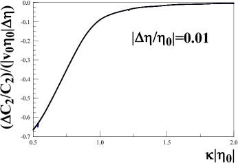
Figure 3: $(\Delta C_{2}/C_{2})/|v_{0}\;\eta_{0}\;\Delta|$ vs $\kappa|\;\eta_{0}|$ for the square well potential, for $|v_{0}|\;\eta_{0}^{2}=1,\;3,\;5~{};~{}|\Delta/\eta_{0}|=0.01$ (left panel) and $|\Delta/\eta_{0}|=0.1$ (right panel). There is a substantial suppression of the quadrupole when the potential is localized at a time scale $\eta_{0}\sim 1/[a_{0}\;H_{0}]$. This time scale is approximately $55$ e-folds before the end of inflation when the wavelengths corresponding to today’s Hubble radius exited the horizon.

Figure 4: $(\Delta C_{l}/C_{l})/|v_{0}\;\eta_{0}\;\Delta|$ vs $l$ for the square well potential , for $|v_{0}|\;\eta_{0}^{2}=1;\kappa\;|\eta_{0}|=1$ and $|\Delta/\eta_{0}|=0.01,\;0.1$. We see that the suppresion of higher multipoles are negligibly small (they fall off as $1/l^{2}$) and observationally irrelevant.

These exact results agree remarkably well with the simpler Born approximation within the range of parameters consistent with small number of particles as required by the small backreaction condition. Therefore, this exactly solvable example lends support to the statement that the Born approximation is indeed robust and describes remarkably well the main corrections from the potential $\mathcal{V}(\eta)$.

These results apply equally well to curvature and tensor perturbations. Therefore, this analysis leads to the prediction that the quadrupole of tensor perturbations will also feature a suppression.

VI Conclusions

In this article we studied the effect of initial conditions on metric and tensor perturbations with emphasis on the observational consequences of initial conditions consistent with renormalizability and small backreaction. Generalized initial conditions for the mode functions of gauge invariant perturbations are encoded in Bogoliubov coefficients, or equivalently in distribution functions of Bunch-Davies quanta. We begun the study by clarifying the constraint on the Bogoliubov coefficients from the general restrictions of renormalizability and negligible back reaction on the energy momentum tensor of gauge invariant perturbations. These general criteria constrain the asymptotic behavior for large wave vectors of the Bogoliubov coefficients up to $1/k^{4}$. We find that the modifications to the power spectra of gauge invariant perturbations due to general initial conditions are encoded in a transfer function for initial conditions $D(k)$. Our main results are summarized as follows:

• General arguments based on the asymptotic behavior of the Bogoliubov coefficients at large wave vector show that only the low multipoles, those in the Sachs-Wolfe plateau, are sensitive to initial conditions allowed by renormalizability and small back reaction. Effects upon high multipoles are strongly suppressed by the rapid fall off of the Bogoliubov coefficients at large wavevectors $k$. We compute the change in the quadrupole due to generic initial conditions described by the asymptotic limit of the Bogoliubov coefficients. A substantial change of the order $10-20\%$ on the CMB quadrupole is found when the momentum scale at which the asymptotic behavior sets corresponds to the physical wavelength of the order of the Hubble radius today.

• We show that mode functions with general initial conditions determined before the slow roll stage are equivalent to those that result from scattering by the potential $\mathcal{V}(\eta)$ arising from the cosmological evolution just prior to the onset of slow roll. The influence of initial conditions upon the power spectra of curvature and tensor perturbations is encoded in a transfer function $D(k)$.

• Implementing methods from scattering theory, we develop the formulation of initial conditions arising from scattering by a potential $\mathcal{V}(\eta)$ and obtain the transfer function of initial conditions $D(k)$ in terms of this potential. The changes in the low multipoles are studied both in the Born approximation and in a exact solvable case for $\mathcal{V}(\eta)$, with complete agreement between the results in both cases. The transfer function for initial conditions is shown to have the asymptotic large $k$ behavior consistent with renormalizability and negligible back reaction.

• Furthermore, this study reveals that attractive potentials lead to a suppression of the quadrupole with a value consistent with the WMAP data if the the potential is localized at a time scale $\eta_{0}$ very near the scale at which the wavelength corresponding to the Hubble radius today exits the horizon during inflation, with a strength $\mathcal{V}(\eta_{0})\sim 1/\eta^{2}_{0}$. The change in the $l$-multipole falls off as $1/l^{2}$ as a consequence of the fall off of the Bogoliubov coefficients for large $k$. This entails that only the quadrupole features an observable suppression, while the corrections in higher multipoles are not observable with the present data.

• Our study applies to curvature and tensor perturbations, hence we predict a suppression of quadrupole for B-modes for an attractive potential localized prior to slow roll.

In the companion article II we show that the potential $\mathcal{V}(\eta)$ which determines the initial conditions for the fluctuations in the slow roll stage is a general feature of a stage of fast roll inflaton dynamics followed by slow roll. Under general circumstances this potential turns out to be attractive and results in a suppression on the CMB quadrupole of the order $\sim 10-20\%$ consistent with the observations.

- (1) D. Kazanas, ApJ 241, L59 (1980); A. Guth, Phys. Rev. D23, 347 (1981); K. Sato, MNRAS, 195, 467 (1981).
- (2) E. W. Kolb, M. S. Turner, The Early Universe Addison Wesley, Redwood City, C.A. 1990.
- (3) P. Coles , F. Lucchin, Cosmology, John Wiley, Chichester, 1995.
- (4) A. R. Liddle, D. H. Lyth, Cosmological Inflation and Large Scale Structure, Cambridge University Press, 2000; Phys. Rept. 231, 1 (1993) and references therein.
- (5) D. H. Lyth, A. Riotto, Phys. Rept. 314, 1 (1999).
- (6) A. A. Starobinsky, JETP Lett. 30, 682 (1979). V. F. Mukhanov, G. V. Chibisov, Soviet Phys. JETP Lett. 33, 532 (1981).
- (7) V. F. Mukhanov, H. A. Feldman , R. H. Brandenberger, Phys. Rept. 215, 203 (1992).
- (8) J. E. Lidsey et al. Rev. Mod. Phys. 69, 373 (1997).
- (9) A. Riotto, hep-ph/0210162.
- (10) M. Giovannini, Int. J. Mod. Phys. D14 363 (2005).
- (11) C. L. Bennett et.al. (WMAP collaboration), Astro. Phys. Jour. Supp. 148, 1 (2003).
- (12) E. Komatsu et.al. (WMAP collaboration), Astro. Phys. Jour. Supp. 148, 119 (2003).
- (13) D. N. Spergel et.al. (WMAP collaboration), Astro. Phys. Jour. Supp. 148, 175 (2003).
- (14) A. Kogut et.al. (WMAP collaboration) Astro. Phys. Jour. Supp. 148, 161 (2003).
- (15) H. V. Peiris et.al. (WMAP collaboration), Astro. Phys. Jour. Supp. 148, 213 (2003).
- (16) D. N. Spergel et.al. (WMAP collaboration), astro-ph/0603449.
- (17) L. Page et.al. (WMAP collaboration), astro-ph/0603450.
- (18) G. Hinshaw et. al. (WMAP collaboration), astro-ph/0603451.
- (19) T. S. Bunch and P. C. Davies, Proc. R. Soc. A360, 117 (1978); N. D. Birrell and P. C. W. Davies, Quantum fields in curved space, (Cambridge Monographs in Mathematical Physics, Cambridge University Press, Cambridge, 1982).
- (20) A. Vilenkin and L. H. Ford, Phys. Rev. D26, 1231 (1982); A. D. Linde, Phys. Lett. 116B, 335 (1982); A. A. Starobinsky, Phys. Lett. 117B, 175 (1982). E. Mottola, Phys. Rev. D31, 754 (1985). B. Allen, Phys. Rev. D32, 3136 (1985).
- (21) P. R. Anderson, C. Molina-Paris, E. Mottola, Phys. Rev. D72, 043515 (2005); S. Habib, C. Molina-Paris and E. Mottola, Phys. Rev. D61, 024010 (2000); P. R. Anderson, W. Eaker, S. Habib, C. Molina-Paris, E. Mottola, Phys. Rev. D62, 124019 (2000).
- (22) R. H. Brandenberger and J. Martin, Mod. Phys. Lett. A16, 999 (2001); Int. J. Mod. Phys. A17, 3663 (2002); Phys. Rev. D71, 23504 (2005); J. Martin and R. H. Brandenberger, Phys. Rev. D63, 123501 (2001); D65 103514 (2002); D68, 63513 (2003); R. H. Brandenberger, S. E. Joras, and J. Martin, Phys. Rev. D 66, 83514 (2002); R. Easther, B. R. Greene, W. H. Kinney, and G. Shiu, Phys. Rev. D 64, 103502 (2001); D66, 23518 (2002); D67, 63508 (2003); G. Shiu and I. Wasserman, Phys. Lett. B536, 1 (2002); C. P. Burgess, J. M. Cline, F. Lemieux, and R. Holman, JHEP 302, 48 (2003); C. P. Burgess, J. M. Cline, and R. Holman, JCAP 310, 4 (2003); U. H. Danielsson, Phys. Rev D66, 23511 (2002); L. Bergstrom and U. H. Danielsson, JHEP 212, 38 (2002); U. H. Danielsson, JHEP, 207, 40 (2002); 212, 25 (2002); T. Tanaka, astro-ph/0012431; N. Kaloper, M. Kleban, A. Lawrence, S. Shenker, Phys. Rev. D66, 123510 (2002); L. Hui and W. H. Kinney, Phys. Rev. D65, 103507 (2002); L. Mersini, M. Bastero-Gil, and P. Kanti, Phys. Rev. D64, 043508 (2001); J.C. Niemeyer, Phys. Rev. D63, 123502 (2001); A. Kempf and J.C. Niemeyer, Phys. Rev. D64, 103501 (2001); A. A. Starobinsky, JETP Lett. 73, 415 (2001); M. Lemoine, M. Lubo, J. Martin, and J.-P. Uzan, Phys. Rev. D65, 023510 (2001); M. Lemoine, J. Martin, and J.-P. Uzan, Phys. Rev. D67, 103520 (2003); F. Lizzi, G. Mangano, G. Miele, M. Peloso, JHEP 0206, 049 (2002); N. Kaloper, M. Kleban, A. Lawrence, S. Shenker, and L. Susskind, JHEP 211, 37 (2002); A. A. Starobinsky and I. I. Tkachev, JETP Lett. 76, 235 (2002); M. Bastero-Gil and L. Mersini, Phys. Rev. D67, 103519 (2003); J. C. Niemeyer, R. Parentani, and D. Campo, Phys. Rev. D66, 83510 (2002); V. Bozza, M. Giovannini, and G. Veneziano, JCAP 305, 1 (2003); M. Porrati, Phys. Lett. B 596, 306 (2004); B. R. Greene, K. Schalm, G. Shiu, and J. P. van der Schaar, JCAP 502, 1 (2005); U. H. Danielsson, Phys. Rev. D71, 23516 (2005) and astro-ph/0606474; H. Collins and R. Holman, Phys. Rev. D71, 085009 (2005); M. Giovannini, Class.Quant.Grav. 20 (2003) 5455; H. Collins and R. Holman, hep-th/0605107. L. Covi et al., astro-ph/0606452. C. Doran, A. Lasenby, Phys. Rev. D71, 063502 (2005).
- (23) G. F. Smoot et. al. (COBE collaboration), Astro. Phys. Jour. 396, 1 (1992).
- (24) A. de Oliveira-Costa, M. Tegmark, M. Zaldarriaga and A. J. Hamilton, Phys. Rev. D69, 063516 (2004); G. Efstathiou, Mon. Not. Roy. Astron. Soc. 348 885 (2004); E. Gaztanaga et. al. Mon. Not. Roy. Astron. Soc. 346, 47 (2003).
- (25) C. J. Copi, D. Huterer, and G. D. Starkman, Phys. Rev. D70, 043515 (2004); D. Schwarz, G. Starkman, D. Huterer and C. Copi, Phys. Rev. Lett. 93, 221301 (2004); C. Copi, D. Huterer, D. Schwarz and G. Starkman, arXiv: astro-ph/0508047; K. Land and J. Magueijo, Phys. Rev. Lett. 95, 071301 (2005 ); Mon. Not. Roy. Astron. Soc. 362, 838 (2005); C. Copi, D. Huterer, D. Schwarz, and G. Starkman, astro-ph/0605135; F. Hansen, P. Cabella, D. Marinucci and N. Vittorio, Astrophys. J. 607, L67 (2004); H. Eriksen, F. Hansen, A. Banday, K. Górski and P. Lilje, Astrophys. J. 605: 14 (2004).
- (26) N J Cornish, D N Spergel, G D Starkman, E Komatsu, Phys.Rev.Lett. 92, 201302 (2004); B F Roukema, B Lew, M Cechowska, A Marecki, S Bajtlik, Astronomy and Astrophysics 423, 821 (2004); W S Hipolito-Ricaldi, G I Gomero, astro-ph/0507238; J G Cresswell, A R Liddle, P Mukherjee, A Riazuelo ;Phys.Rev. D 73,041302 (2006); M J Reboucas, J S Alcaniz 2006, astro-ph/0603206; B. Feng, M. Li, R-J Zhang, X. Zhang, Phys.Rev. D68,103511 (2003); P. G Castro, M. Douspis, P. G. Ferreira 2003; Phys.Rev. D68,127301 (2003); C. J. Hogan,Phys.Rev.D70,083521 (2004); N. Kaloper, Phys.Lett. B583,1 (2004); M. Liguori, S Matarrese, M Musso, A Riotto, JCAP 408, 011 (2004); C. J. Hogan, astro-ph/0406447; R. V. Buniy 2005; Int. J. Mod. Phys. A20,1095 (2005); P. Hunt, S. Sarkar 2004; Phys.Rev.D70,103518 (2004); A. Linde, JCAP 410,004 (2004); R. V. Buniy, A. Berera, T. W. Kephart, hep-th/0511115; A. Kostelecky Phys.Rev.D69,105009 (2004); T. Multamaki, O. Elgaroy, Astronomy and Astrophysics 423,811 (2004); C. Gordon, W. Hu, Phys.Rev. D70,083003 (2004); J. W. Moffat, JCAP 510,012 (2005); T. R. Jaffe, A. J. Banday, H. K. Eriksen, K. M. Gorski, F. K. Hansen, ApJ.629, L1 (2005); L. Knox, astro-ph/0503405; C. Gordon, W. Hu, D. Huterer, T. Crawford, Phys.Rev. D72,103002 (2005); P. Jain, M. S. Modgil, J. P. Ralston, astro-ph/0510803; C-H. Wu, K.-W. Ng, W. Lee, D.-S. Lee, Y.-Y. Charng, astro-ph/0604292. S. Cremonini, Phys.Rev. D68, 063514 (2003). L. Campanelli, P. Cea, L. Tedesco, Phys. Rev. Lett. 97, 131302 (2006). Y. Shtanov, V. Sahni, Phys. Lett. B557, 1 (2003). Y. S. Piao, Phys. Rev. D71, 087301 (2005). M. Kawasaki, F. Takahashi, Phys. Lett. B570, 151 (2003). R. Allahverdi, K. Enqvist, J. Garcia-Bellido, A. Mazumdar, hep-ph/0605035.
- (27) A. de Oliveira-Costa and M. Tegmark, Phys.Rev. D74 (2006) 023005.
- (28) L. R. Abramo, L. Sodre Jr, C. A. Wuensche, astro-ph/0605269.
- (29) D. Boyanovsky, H. J. de Vega, N. G. Sanchez, Phys. Rev. D 73, 023008 (2006).
- (30) D. Boyanovsky, H. J. de Vega, N. G. Sanchez, astro-ph/0607487.
- (31) D. Cirigliano, H. J. de Vega, N. G. Sanchez, Phys. Rev. D 71, 103518 (2005). H. J. de Vega, N. G. Sanchez, astro-ph/0604136.
- (32) L. R. Abramo, R. H. Brandenberger and V. F. Mukhanov, Phys. Rev. D56, 3248 (1997); L. R. Abramo, Ph. D. Thesis, gr-qc/9709049.
- (33) D. Boyanovsky, H. J. de Vega, N. G. Sanchez, Phys. Rev. D72 103006, (2005).
- (34) M. Giovannini, Class. Quan. Grav. 20 5455 (2003).
- (35) Handbook of Mathematical Functions, M. Abramowitz and I. A. Stegun, NBS, Washington, 1970.