On the dipole straylight contamination in spinning space missions dedicated to CMB anisotropy
Abstract
We present an analysis of the dipole straylight contamination (DSC) for spinning space-missions designed to measure CMB anisotropies. Although this work is mainly devoted to the Planck project, it is relatively general and allows to focus on the most relevant DSC implications. We first study a simple analytical model for the DSC in which the pointing direction of the main spillover can be assumed parallel or not to the spacecraft spin axis direction and compute the time ordered data and map. The map is then analysed paying particular attention to the DSC of the low multipole coefficients of the map. Through dedicated numerical simulations we verify the analytical results and extend the analysis to higher multipoles and to more complex (and realistic) cases by relaxing some of the simple assumptions adopted in the analytical approach. We find that the systematic effect averages out in an even number of surveys, except for a contamination of the dipole itself that survives when spin axis and spillover directions are not parallel and for a contamination of the other multipoles in the case of complex scanning strategies. In particular, the observed quadrupole can be affected by the DSC in an odd number of surveys or in the presence of survey uncompleteness or over-completeness. Various aspects relevant in CMB space projects (such as implications for calibration, impact on polarization measurements, accuracy requirement in the far beam knowledge for data analysis applications, scanning strategy dependence) are discussed.
keywords:
Cosmology: cosmic microwave background – space vehicles: instruments – methods: data analysis.1 Introduction
The observed pattern of the cosmic microwave background (CMB) anisotropies is dominated by the dipole signal originating from the motion of the Sun in the CMB rest frame. This signal is two orders of magnitude larger than the typical cosmological effect. While the dipole subtraction is of primary importance to map CMB anisotropies, little is known about the straylight contamination induced by this dipole pattern. The straylight contamination consists in unwanted radiation entering the beam at large angles from the antenna boresight direction. The most relevant contribution is expected from a particular far beam extended region, the so-called main spillover, typically located at from the main optical axis. In the case of the Planck 111http://www.rssd.esa.int/planck telescope, its peak response is at from the telescope optical axis (Sandri et al., 2004) and points far away from the Sun along directions not far from the spacecraft spin axis. It is already known that the straylight contamination of other non-cosmological effects, such as Galactic emissions (Burigana et al., 2001a, 2004; Sandri et al., 2004) and inner Solar System bodies (Burigana et al., 2000, 2001b), plays an important role in designing space-missions like Planck (Mandolesi et al., 1998, 2002; Puget et al., 1998; Lamarre et al., 2002; Tauber, 2001, 2006). Its control and removal represents also a relevant aspect of WMAP 222http://lambda.gsfc.nasa.gov/product/map/current/ design and data analysis (Barnes et al., 2003; Jarosik et al., 2006).
The aim of this paper is to study the dipole straylight contamination (DSC) with analytical and numerical methods. We start building a model sufficiently simple to be treated analytically that allows to understand to first order how the straylight features affect the recoverd CMB angular power spectrum in a way largely independent of the specific optical and scanning strategy details. The analysis is first performed considering the direction of pointing of the main spillover centre parallel or not to the spin axis but keeping the the main spillover centre direction in the plane defined by the telescope and spin axis directions. In this work, we call the angle between the main spillover centre direction and the spin axis direction. We then extend the analysis allowing for displacements of the main spillover centre direction from the plane defined by the telescope axis and the spin axis. The analytical results are presented perturbatively in .
We shall work in the fixed frame with the satellite with axes pointing fixed (far away) stars. In this frame the vector associated to the dipole is constant while the main spillover direction is not (it rotates of in year). We consider the dipole for the motion of the Sun with respect to the rest frame of the CMB and we neglect, for simplicity, small deviations due to the motion of the Earth around the Sun.
We implement dedicated numerical simulations in order to check the analytical results and extend the analysis to more complex (and realistic) cases by relaxing some of the simple assumptions adopted in the analytical approach. In particular, simulations allow to consider non-small values of the angle and complicate scanning strategies introducing the effect associated to the survey uncompleteness (or over-completeness) and extending the analysis to higher multipoles, .
Finally we discuss how the DSC may affect the multipole pattern, with particular emphasis paid to the possible connection with the small signal observed by COBE/DMR (Hinshaw et al., 1996) and WMAP (Bennett et al., 2003a; Spergel et al., 2003, 2006) at low .
The article is organized as follows. In Section 2 the convolution of the dipole and the straylight beam is presented. The analytical model for the beam response in the main spillover region is presented in Section 3 where the map is computed with particular care to low multipoles (up to ). In Section 4 the power spectrum is discussed and the DSC of the quadrupole () is analysed. In Section 5 numerical simulations are presented and discussed. In Section 6 we extend the analysis to arbitrary directions of the main spillover. The main implications for spinning space missions dedicated to the CMB anisotropy are discussed in Section 7. In Section 8 a statistical analysis for the amplitude of the quadrupole is presented. Finally, our main conclusions are drawn in Section 9.
2 The dipole and the straylight beam
We start considering the convolution of the dipole with the main spillover:
| (2.1) |
where is the element of solid angle, with the colatitude and the longitude , the sum on over is understood, are the coefficients of the expansion of the dipole 333We use the symbol because we want to make clear that the dimensionality is given by a temperature (e.g. in K). on the basis of the spherical harmonics , and is the beam response representing the shape of the main spillover in the -plane. In this notation is normalized to the whole beam integrated response, dominated by the contribution in the main beam
| (2.2) |
where , with 444FWHM = Full Width Half Maximum. representing the main beam angular resolution.
The convolution can be rewritten in the following way:
| (2.3) |
where is the real part of . In order to obtain equation (2.3) it has been used that , where the symbol ⋆ means complex conjugation. For sake of completeness, we write the spherical harmonics for (Sakurai, 1985):
| (2.4) | |||
| (2.5) |
Although it may not be clear from the notation of equation (2.3), notice that is a function of the geometric features of the shape of the main spillover in the -plane.
3 Analytical models
Equation (2.3) is general and exact. Any specific approximation of the beam response inspired by experiments will introduce a certain degree of uncertainty with respect to the real case. We introduce two different parametrizations for : we first consider the Top Hat approximation, analysed in Subsection 3.1, and then the Gaussian approximation, studied in Subsection 3.2. We shall see in the following that the two descriptions are quite similar and are formally equivalent when the main spillover area is sufficiently small (see Subsection 3.3). For this reason we concentrate on the Top Hat case for the analytical estimate of the DSC.
3.1 Top hat approximation
Our first approximation (Gruppuso, Burigana & Finelli, 2005) for is the Top Hat:
| (3.1) | |||
where is a constant (that is related to the ratio between the power entering the spillover and the power entering the main beam and it is a number much less than – it will be estimated in Subsection 4.1) and is the step function (or Heaviside function) that takes the value for and the value otherwise. Equation (3.1) is just an asymmetrical rectangular box, in the -plane, centred around the point and with sides of length and . Notice that the point is the direction of pointing of the main spillover centre. This approximation leads to:
| (3.2) |
Considering that
with and implicitely defined by and , we obtain the final expression for the convolution:
| (3.3) |
where the label TH stands for Top Hat. Here we have made the notation lighter setting and . If the box is centred (i.e. and ) and the direction of the main spillover coincides with the spin axis [i.e. ], then the convolution is (Gruppuso, Burigana & Finelli, 2004)
| (3.4) |
where we have made explicit the dependence on time for . Notice that the term proportional to drops out in this simple case.
3.2 Gaussian approximation
The Gaussian approximation can be described rescaling the dipole signal as
| (3.5) |
where the factor is the Gaussian window function, , specified at and is the FWHM for the main spillover divided by , and adopting as main spillover response
| (3.6) |
where (as before) is related to the ratio between the power entering the main spillover and the power entering the main beam. In fact equation (3.6) is a pencil beam while the above rescaling of mimics the convolution of the dipole with a Gaussian beam. In this way it is easy to compute the following Gaussian convolution
| (3.7) |
3.3 Link between top hat and Gaussian formalism
We shall see in Subsection 3.4 that we are interested in the following directions for the mainspillover
| (3.8) | |||
| (3.9) |
Replacing equations (3.8) and (3.9) in equation (3.3) and considering a symmetrical top hat (i.e. and ), one obtains the following expression
| (3.10) |
where only the linear term in is kept. Inserting equations (3.8) and (3.9) in equation (3.7) and expanding in again to the linear order one finds
| (3.11) | |||
Equation (3.10) and equation (3.11) are very similar and become the same expression for small , if we define as follows
| (3.12) |
This is an intuitive result: up to normalizations, a pencil beam and a top hat beam are not distinguishable when the (angular) area for the top hat is sufficiently small. Given this result, in the following analytical treatment we will focus, for sake of compactness, only on the symmetrical top hat case adopting
| (3.13) | |||
| (3.14) |
in the numerical estimates. Instead, we will widely consider the Gaussian case in the section dedicated to the numerical simulations.
3.4 Relation between main beam and main spillover
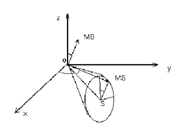
During the rotation of the main beam, the main spillover, if not lying on the spin axis, draws a cone, as depicted in Figure 1. This means that the direction of the main spillover and of the main beam are related by
| (3.15) | |||
| (3.16) |
where is the colatitude of the main beam, is the angle at the vertex of the cone and is the longitude of the spin axis (see also caption of Figure 1). The upper (lower) sign of equation (3.16) has to be taken into account when the main beam rotates from North (South) to South (North).
In order to make realistic this simple model, we have to check that during the rotation, the solid angle, subtended by the main spillover (), is constant. A simple calculation gives
| (3.17) |
Of course equation (3.17) is not constant because is a function which depends on time. However, we have
| (3.18) |
and therefore is constant in time to linear order in . This means that the analytical calculation will be done to linear order in . Then equations (3.15) and (3.16) will be Taylor expanded for small , obtaining
| (3.19) | |||
| (3.20) |
3.5 Building the map
The total signal received by the satellite receiver, is the sum of the two following terms:
| (3.21) |
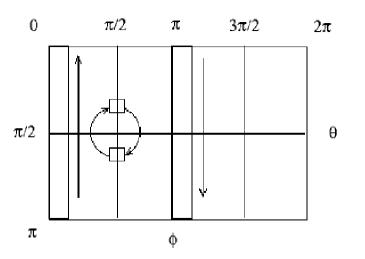
here is the signal entering the main beam (where the dipole has been subtracted away) whereas is the signal due to the dipole entering the main spillover. We take into account for simplicity a simple scanning strategy as that considered in the Planck project as nominal scanning strategy (NSS) (Dupac & Tauber, 2005), i.e. with the spacecraft spin axis always in the antisolar direction or, in practice, always on the ecliptic plane as valid when the small effect of the spacecraft orbit around the Lagrangian point L2 of the Sun-Earth system is neglected.
In this case, for the first survey is given by
| (3.27) |
whereas, for the second survey it is
| (3.33) |
The shift in the definition of the arguments in (during either the first or the second survey) comes from the fact that when the main beam rotates from North to South the main spillover is shifted of plus a small correction proportional to (due to the non-perfect alignment of the main spillover with the spin axis), while when the main beam rotates from South to North the main spillover is shifted of minus a small correction proportional to (still due to the non-perfect alignment of the main spillover with the spin axis). Moreover note that it has been used that when the main beam rotates from North to South while when the main beam rotates from South to North. See Figure 2 for a sketch of the scanning.
Notice that now is the pointing of the main beam (we omitted the label to make the notation lighter).
3.6 Definition of
As usual, we expand the signal in spherical harmonics
| (3.34) |
which implies
| (3.35) |
We consider the multipole expansion of the straylight contribution
| (3.36) |
To make lighter the notation, we rewrite the convolution in a compact form as
| (3.37) |
with
| (3.38) | |||
| (3.39) | |||
| (3.40) | |||
| (3.41) | |||
| (3.42) |
3.7 General results after an odd number of surveys
After one or an odd number of surveys it is possible to show that all the with odd vanish when , as follows from:
| (3.43) |
where the label 0 stands for and where the label SL has been dropped for simplicity. Changing variable of integration [ in the first integration and in the second integration of equation (3.43)] and considering that
| (3.44) |
then equation (3.43) reads
| (3.45) |
Equation (3.45) is identically satisfied when is even and demands when is odd.
Moreover, still considering equation (3.43), the integration over vanishes when is odd with respect to . This happens when is odd and is even 555 is odd with respect to also when is even and is odd., i.e. :
| (3.46) |
Equations (3.45) and (3.46) show that only with even and even, can be non-vanishing. In particular if is odd, a property that will be widely used throughout the article.
Considering small but not zero then is possible to write as follows
| (3.47) |
where the label 1 stands for first order in . It turns out that
| (3.48) |
where . For symmetry reasons it is possible to show that only
| (3.49) |
and
| (3.50) |
can be different from zero when is odd. It turns out that both equations (3.49) and (3.50) vanish except the case . We calculate
| (3.51) |
and
| (3.52) |
This means that the unique term that turns on (linearly in ) when is taken different from zero (and small) is the dipole term. All the other terms deviates from results at least for .
3.8 Surviving systematic effect after an even number of surveys
After two (or an even number of) surveys the average
| (3.53) |
where the labels (I) and (II) stand for first and second survey respectively, is different from zero only for (to the linear order in ). This term vanishes when . This means that the whole effect averages to when .
In order to show this statement, consider that with replacements similar to the ones performed in Subsection 3.7 one obtains
| (3.54) |
where turns out to be the same integral given in equation (3.48) and studied in the Subsection 3.7. Notice that the average over two surveys is equivalent to one survey result.
This demonstrates the statement made at the beginning of this Subsection 666The fact that DSC has null average after surveys when can be shown also integrating over the time interval corresponding to surveys..
3.9 The computation of
In Subsection 3.7 it has been shown that the calculation of to linear order in is equivalent to the one with (i.e. ) if we exclude the case . Moreover in order to have the possibility of obtaining a non-vanishing , we must constrain and to be even.
3.9.1
Specifying and we obtain
| (3.55) |
The monopole deviates from the order as .
3.9.2
Specifying and we obtain
| (3.56) |
For and we have
| (3.57) |
Equations (3.56) and (3.57) show that only in the simplified case in which the spin axis is parallel to the direction of the main spillover (i.e. ), we have that the DSC map does not show dipole contribution 777We will see in Subsection 5.2.1 that equations (3.56) and (3.57) can be generalized for non-small substituting with .. This could have some important consequences on calibrations based on the kinematic dipole. It is interesting to note that this contribution survives even after two surveys. This is the unique contribution that does not average to zero (when ) after an even number of surveys.
3.9.3
Specifying and , it is easy to obtain
| (3.58) |
implying that it is vanishing at linear order in . Notice that even if symmetry arguments would make possible a contribution (i.e. and are both even) at the order in , the result is vanishing. As it is already known from Subsection 3.7 for :
| (3.59) |
where no expansion in has been performed in order to obtain this result. For :
| (3.60) |
where does not appear to linear order [there are corrections of order ].
These results have been computed using the definition of spherical harmonics for , that we report here for sake of completeness (Sakurai, 1985):
| (3.61) | |||
| (3.62) | |||
| (3.63) |
Equation (3.60) is the (non-vanishing) contribution to the quadrupole due to the dipole entering the straylight. This is one of the main result of this work.
3.9.4
Setting , and , we obtain:
| (3.64) |
Notice that even if symmetry arguments do not prevent a contribution, for and , nevertheless the computation gives . For :
| (3.65) |
For :
| (3.66) |
For :
| (3.67) |
These results have been computed using the definition for of spherical harmonics for , that we report here for sake of completeness (Sakurai, 1985):
| (3.68) | |||
| (3.69) | |||
| (3.70) | |||
| (3.71) | |||
| (3.72) |
4 Impact on the Angular Power Spectrum
The quadrupole presents a contamination that does not depend on (to the order we are performing the computation). In this Section we perform a detailed analysis of this effect.
4.1 Comparison among with low
We consider
| (4.1) |
where is the relative power entering the main spillover with respect to the total one (i.e. essentially entering the main beam). By the definition of ,
| (4.2) |
we compute
| (4.3) |
| (4.4) |
| (4.5) |
| (4.6) |
where
As an example, we choose and . Moreover it is possible to show that
| (4.7) | |||
| (4.8) | |||
| (4.9) |
where is the direction and is the amplitude of the dipole 888These relations are obtained solving the following set of equations , and . Of course, the solution can be verified replacing in ..
In ecliptic coordinates, according to WMAP (Bennett et al., 2003a), and . We then obtain:
| (4.10) | |||
| (4.11) | |||
| (4.12) |
Now we give, as an axample, some numerical results. We have
| (4.13) | |||
| (4.14) | |||
| (4.15) |
and for
| (4.16) |
while for
| (4.17) |
4.2 The angular power spectrum
From equations (3.21) and (3.35) it is clear that:
| (4.18) |
where is already defined in equation (3.36) and is
| (4.19) |
The CMB power spectrum is given by
| (4.20) |
and replacing equation (4.18) one obtains
| (4.21) | |||||
In particular for the quadrupole we have
| (4.22) |
and
| (4.23) |
where it has been used and , with defined as
| (4.24) | |||||
From equation (4.24), choosing and considering we have .
4.3 DSC of the quadrupole
We are ready to estimate the order of magnitude of and . Since are stochastic numbers with vanishing mean and standard deviation equal to , we adopt, as an example, the following relation
| (4.25) |
for numerical estimate, where the factor 2 is due to the assumption that the real and imaginary part give the same contribution 999This choice on the real and imaginary part of is limited to this Subsection. In Section 8 a statistical analysis will be performed.. We obtain:
| (4.26) |
| (4.27) |
where it has been chosen . The in equation (4.27) is due to our ignorance about the relative sign of and .
| SL | ||||
| SKY-SL | ||||
| SL | ||||
| SKY-SL | ||||
| SL | ||||
| SKY-SL |
In Table 1 there are and for and . All the numbers for contribution have to be understood with a in front of them (since we do not know the total sign of this contribution).
We stress two main observations. First, we notice that the contribution is smaller than the contribution if is sufficiently small. This is clear because is quadratic in while is linear. Therefore, for and we have that the leading term is given by while for we find that is subleading; second, since contribution is always positive, because of the previous observation, it is clear that can be lowered only for the first and second column of Table 1, when the relation (4.25) is chosen.
4.4 Decrease of the quadrupole
From equation (4.21) we can rewrite the observed quadrupole as a function of
| (4.28) |
where
| (4.29) | |||
| (4.30) |
Equation (4.28) is just a parabolic behaviour in with concavity in the upward direction since the coefficient of is always positive. The sign of is not known a priori: from equation (4.23) or equation (4.28) is clear that can decrease only if . We focus now on this case.
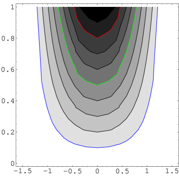
The minimum value is reached by the vertex , , where
| (4.31) | |||
Considering that , we can rewrite equation (4.31) as
| (4.32) |
where (then ) and with being the norm of the vector ,
| (4.33) |
and with defined as
| (4.34) |
and therefore ranging in the set . In Figure 3 we show a contour plot for the ratio versus the couple of parameters . Darker is the grey and smaller is the ratio (see also the caption).
In the same way we rewrite equation (4.28) as
| (4.35) | |||||
| (4.36) |
This means that the first branch of DSC is given by (where also a decreasing of the observed quadrupole is possible, i.e. ) and the second branch is given by (where only an increasing of the observed quadrupole is possible, i.e. ). In Figure 4 we plot equation (4.35) for (red, green, blu and yellow lines respectively) with (lower curves) and with (upper curves).
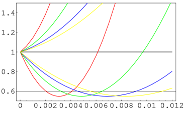
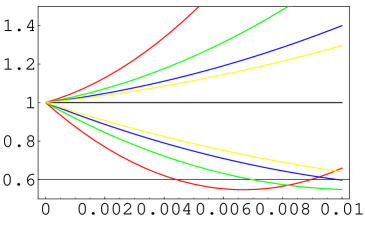
Bottom panel of Figure 4 is a zoom of the top panel but with as independent variable instead of (see also the caption).
5 Numerical Simulations
The results presented in the previous sections are based on an analytical treatment of the DSC effect. Numerical simulations allow to independently check the analytical results of the previous Section and to extend the analysis to more complex (and realistic) cases by relaxing some of the simple assumptions adopted in the previous sections. In particular, we will investigate through dedicated computations some aspects that are difficult or impossible to address in analytical way: i) the case of a non-small angle (i.e. of a deviation of some tens of degrees from the orthogonality between the directions of the main beam and the main spillover); ii) more complicate scanning strategies including, for instance, precessions of the spacecraft spin axis around the nominal case of a spin axis direction kept along the antisolar direction, i.e. in practice on the ecliptic plane. Moreover, simulations allow to take into account iii) the effect introduced by the uncompleteness of one of the two surveys and iv) to extend the analysis to higher multipoles in the cases i) and ii).
 |
 |
 |
 |
 |
 |
 |
 |
5.1 The numerical code
We used here an update dedicated version of the code implemented and successfully tested in many simulation works devoted to the study (and reduction) of various classes of systematic effects in the context of the Planck mission under different scanning strategy assumptions. It is described in detail in Burigana et al. (1998) and Maino et al. (1999) and, in particular regarding the straylight effect, in Burigana et al. (2001a, 2004), where further informations on the relevant reference systems adopted in the code can be found. We do not consider here the impact of the spacecraft orbit (around the Lagrangian point L2 of the Sun-Earth system, as for example in the case of WMAP and Planck) because its effects are not relevant in this context.
In this work, we compute the convolutions between the main spillover response and the sky dipole signal as described in Burigana et al. (2001a, 2004), but by pixellizing the sky at resolution 101010The HEALPix scheme (http://healpix.jpl.nasa.gov/) by Górski et al. (2005) has been adopted in simulations. A dipole input map at has been considered., considering spin-axis shifts of every day and 396 samplings per scan circle, and by adopting the analytical Gaussian description of the main spillover response introduced in Section 3.2 111111This is certainly a simple approximation of the complexity of the realistic shapes predicted for the main spillover (and in general for the beam response far from the main beam) by optical simulation codes (see e.g. Sandri et al. (2004)). On the other hand, the details of the main spillover response shape depend on the considered optical system. In the context of the Planck activities, they will be included in a future work. The main contribution of this paper is in fact the understanding of the most relevant effects introduced by the DSC, common to relatively different optical systems, in terms of simple parametrizations. that has been explicitely implemented in this version of the code.
We consider here as reference case a channel at 70 GHz, a frequency where the foreground contamination at large angular scales is minimum (Bennett et al., 2003b; Page et al., 2006), and report simulation results in terms of antenna temperature, as typical in simulation activity being it an additive quantity with respect to the sum of various contributions. For numerical estimates, we report here the results referring to the case (i.e. a relative power of 1% entering the main spillover) and assume a main spillover FWHM, FWHMms, of , an angular size amplitude comparable to those of CMB space experiments (Sandri et al., 2004; Barnes et al., 2003).
The adopted resolution allows us to investigate the DSC effect on angular scales larger than few degrees, i.e. up to multipoles , where the most relevant effects are expected because of the large scale features considered here both for the signal and the main spillover response. The main output of the simulation code consists of time ordered data (TOD) containing the signal entering the main spillover for each simulated pointing direction. We generate TOD for two complete sky surveys. The TOD are then coadded to produce all sky maps of DSC at a resolution of ( in the HEALPix scheme). These maps are analysed in terms of angular power spectrum (APS) by using the anafast facility of the HEALPix libraries. For simplicity, we considered always an angle of between the directions of the spacecraft spin axis and of the main beam centre (assumed to be aligned with the telescope line of sight). This assumption allows to reach the all sky coverage for the whole set of considered scanning strategies. Differently, in the absence of spin axis displacements from the ecliptic plane a small unobserved circular patch appears around each of the ecliptic poles (Dupac & Tauber, 2005). We prefer to avoid the case of non-complete sky coverage because it may generate a certain complication in the APS analysis, introducing a mix between the effects from DSC and partial sky coverage. Of course, this choice allows also to check the analytical results in the same work condition.
Our general results are obviously not significantly dependent on the specific choice for FWHMms. In addition, they can be easily rescaled to any value of (signal , APS ).
Finally, we note that the discretization of adopted in the present simulations implies a typical numerical error amplitude significantly less (because of averaging) than K, a value at least one or two order of magnitude smaller than those relevant in this analysis, and then fully negligible for the present purposes.
 |
 |
 |
 |
5.2 Numerical results
We carried out the simulation described in the previous section for various scanning strategies and configurations.
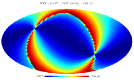
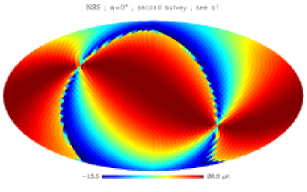
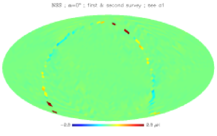
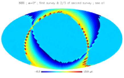
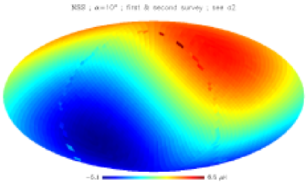
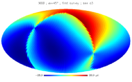
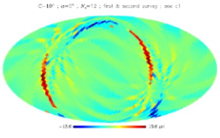
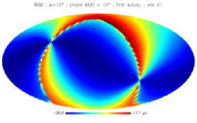
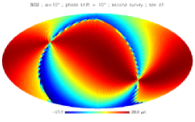
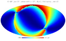
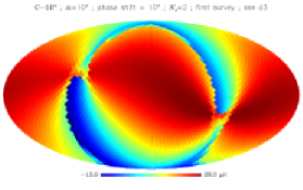
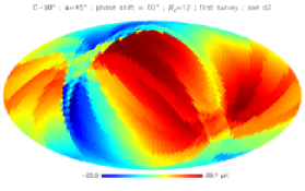
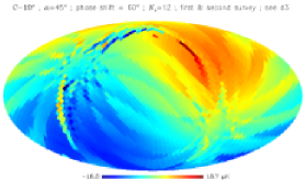
First, we considered the scanning strategy (the NSS) previously adopted in Section 3 with the spin axis always in the antisolar direction for three choices of the angle : and . The corresponding maps for some representative cases are shown in Figures 5 and 6. We considered the maps obtained coadding the TOD from each of the two surveys separately and from the two surveys together. In the case with we considered also the maps obtained from one whole survey plus a second uncomplete (2/3) survey.
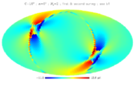
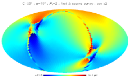
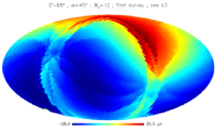
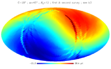
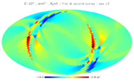
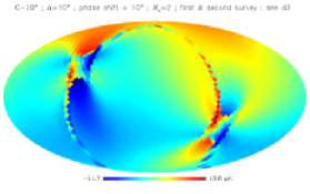
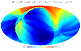
We then considered a cycloidal scanning strategy (C) with periods of 6 months (i.e. a number, , of complete cycloids per 360 days equal to 2), 2 months (i.e. ), and 1 month (i.e. ). The corresponding maps for some representative cases are shown in Figures 6 and 7. In the cases with , we considered and ; in the cases with , we considered and ; in the cases with , we considered . The semi-amplitude of the precession cone has been set to . For comparison, we considered also a semi-amplitude of in the case and . Again, we analysed the cases of each of the two surveys separately and of the two surveys together.
We observe that it is preferable to first produce the map corresponding to each survey separately and then to construct the combined map from the two surveys as a simple average of the two separate maps. In fact, even a relatively small difference in the number of hits per pixel in the two surveys (generated by a combination of pixel shape and effective observational strategy) can introduce a remarkable spurious unbalance in the average when it is done by jointly treating the TOD from the two surveys 121212Note also that considering a single survey, the numerical error in the TOD quoted above is further dropped by averaging. This is not strictly true by combining two surveys because pixel shape and effective scanning strategy imply a not perfect geometrical symmetry between the TOD from the two surveys and the presence of (very small) residual deviations from the ideal case..
The APS obtained analysing the various maps are reported in Figure 8 for some representative cases. In each of the maps in Figures 5, 6, 7 we report the corresponding panel in Figure 8.


|
5.2.1 Simple scanning strategies
The simple view to the maps obtained in the case of the NSS confirms the results derived through the analytical approach.
Figure 5 clearly shows the quadrupole produced by the dipole straylight contamination when only a single survey is considered. Note that the pattern is symmetrical in the two surveys, as expected.
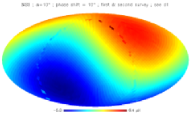
Considering the average of two surveys, the resulting map is essentially zero, except for a small ring, corresponding to the edges of the surveys, where it is in practice impossible to exactly balance the signal from the two surveys as a result of the combination of pixel shape and effective observational strategy.
If one of the two surveys is not complete (see Figure 5), a remarkable quadrupole again appears. Figure 8 clearly shows this effect in terms of APS.
Note that, as expected from the analytical treatment for , our computation gives an APS different from zero only for the even multipoles.
Note also the power decreasing for increasing multipoles. At low multipoles, we have checked that the APS found numerically agrees with the analytical prescription.
Differently from the ideal analytical case, the combination of two complete surveys implies a non-vanishing APS because of small deviations of the exact balance found analytically. In any case, these effect (that is found to decrease by increasing the resolution of the simulation) is absolutely negligible in practice in this context.
Much more remarkable is the APS found when one of the two surveys is not complete. In practice, this may be the case in realistic experiments (even for the most symmetrical NSS) because of the different location of the various receivers on the focal plane. A particular care to this aspect should then be taken in the analysis of low multipoles.
As analytically expected, for a non-negligible dipole contribution also appears, as evident in the map in Figure 6. It has the same amplitude in the two surveys, as predicted. Note that in this case the APS is different from zero also for the odd multipoles, in agreement with the analytical results (see Figure 8). Clearly, the effect is in any case very low, appearing only to higher order in .
For relevant values of , a case that cannot be exhaustively treated through the analytical approach, the power of the dipole and of the other odd multipoles significantly increases (see Figures 6 and 8). Note also in Figure 6 the presence of remarkable features introduced by the significant angle between the directions of the main spillover and of the spacecraft spin axis.
We note that an approximation for the scaling with of the APS with can be derived by the analytical expressions in equations (3.56) and (3.57), holding in the limit of small values , replacing with which implies the dependence evident in panels a2 and a3 of Figure 8. Note also that this dipole scaling holds almost independently of the details of the scanning strategy as clear from panels b2 and b3 of Figure 8 (see also the next subsection), because of its large angular scale origin.
5.2.2 Cycloidal scanning strategies
The complication of the observational strategy implied by a cycloidal option has a clear impact both on the final maps and on the APS.
We first consider slow precessions (6 month period, ). In the case , the most relevant difference with respect to the case of the NSS appears in the combination of the two surveys. As evident in Figure 6, structures appear on various angular scales because of the violation of the balance between the TOD of the two surveys implied by this observational strategy. The APS found in this case (see Figure 8) is similar to that found in the case of the NSS but in the absence of completeness of one of the two surveys.
In the case we find very similar results, except for the expected presence of the dipole and of the other odd multipole terms.
Faster precessions (1 month period) with a significant value of (, see Figures 7 and 8), imply a remarkable dipole signature, analytically expected, a relatively more efficient smoothing of some large scale features in the combination of the two surveys, and then a relative decreasing of the power at multipoles less than with respect to the previous case.
Keeping , we exploit the impact of different precession periods (see Figures 7 and 8). Note in Figure 7 how the precession period appears in the maps as a “finger print”; this effect is evident in general for . This results is analogous to that found for the number of hits in scanning strategy analyses (Dupac & Tauber, 2005), because different precession periods imply different periodic modulations in the dipole amplitude as observed by the main spillover. The comparison between panels b1, c1, c3 in Figure 8 shows that, except for the quadrupole, the first weak and broad low bump in the APS (properly, in terms of ) migrates towards higher multipoles for increasing . This is a direct effect of the decreasing of the angular scale of the “finger print” structures for decreasing precession periods.
Finally, we have investigated on the impact of the precession angle amplitude by considering also an angle of (panel c2 in Figure 8), instead . We find a certain decreasing of the power at multipoles less than 20–30 with respect to the previous cases, in particular jointly considering the two surveys. This can be understood on the basis of a simple continuity argument: decreasing the amplitude, the cycloidal scanning strategy tends to the NSS.
5.2.3 Symmetrical main spillover
For sake of completeness, we have carried out also some simulations assuming a far sidelobe response azimuthally symmetrical with respect to the direction of the main beam 131313This scheme is inspired by the case of observations taken with an antenna pattern similar to that of a feedhorn non-coupled to a telescope.. We assume again a far sidelobe with a Gaussian profile, but in this case this refers only to the dependence on the colatitude from the beam centre axis. We assume again FWHM, but it refers here only to azimuthal cuts. We renormalize the maximum sidelobe response to have again a given ratio (= 0.01 in the current computations) between the sidelobe response integrated over the whole solid angle and the dominant main beam integrated response. In the simulations, we consider two cases, with the maximum sidelobe response located at an angle of from the main beam (i.e. ) or at an angle of from the main beam (i.e. ).
We considered again the NSS and cycloidal modulations of the spin axis, in this case with and a semi-amplitude of .
As expected on the basis of an obvious symmetry argument, in the case we find no effect independently of the adopted scanning strategy.
For increasing , the above full symmetry is broken and in fact in the case we find a non-vanishing effect. On the other hand, the azimuthal symmetry adopted for the far sidelobes implies a strong suppression of the power at multipoles and the only surviving relevant term is the dipole 141414In this case, the far sidelobe azimuthal symmetry, significantly different from that considered in the previous cases, reflects into a suppression of the power at even multipoles and into a presence of a very weak power at odd multipoles, in any case smaller than K2 (and of K2 for ) in terms of , because of high order terms in , analogously to the previous case (again the numerical estimates refer to )., as can easily understood by considering that for the case we recover the case of the original dipole pattern, smoothed and decreased of a factor . The simulations carried out in these cases for show a power at very close to that found in the previous subsections for for the same value of .
 |
 |
 |
 |
 |
 |
 |
 |
 |
6 Displacement of the main spillover
The relaxation of the assumption of main spillover centre location on the plane defined by the spin axis and the telescope line of sight can be easily treated through numerical simulations. Because of the spacecraft rotation about the spin axis, any displacement of the main spillover centre from that plane is geometrically equivalent to a proper phase shift (constant for all scan circles) between the TOD containing the main beam centre pointing directions and the TOD containing the main spillover straylight signals. The TODs from the simulations described in the previous section can be then easily reordered to describe this case.
Figure 9 shows the maps obtained (obviously assuming ) for some representative choices of the relevant parameters while Figure 10 displays the corresponding APS (for instance, the phase shift refers here a “delay” of the main spillover straylight signals).
Note that, as expected, in the case of small values of and of the phase shift the results do not significantly change (see panels d1 and d2 in Figure 10) with respect to the case in which the main spillover centre is located on the plane defined by the spin axis and the telescope line of sight because the leading terms are still those at the lowest order in and in the phase shift, as discussed above. On the contrary, for significant values of and of the phase shift the odd multipole power (not only at ) is similar to that found for the contiguous even multipoles (see panel d3 in Figure 10) for both a single survey and the average of the two surveys 151515In the case of small and significant phase shift we numerically find again that the power at a given even multipole is larger than that at the contiguous odd multipoles (again except at ), although with a mitigation of its dominance, depending on the specific set of considered parameters..

Analytically this phase shift can be parametrized generalizing equations (3.19) and (3.20) as follows
| (6.1) | |||
| (6.2) |
with defining the displacement from and where upper (lower) signs refer to North (South) towards South (North) motion of the main beam. Of course, when is vanishing, equations (3.19) and (3.20) are recovered.
Replacing (6.1) and (6.2) in the definition of [see equation (3.27) or (3.33)] it is possible to compute the map
| (6.3) |
Here is given by equation (3.43) [i.e. the introduction of leaves uneffected the zeroth order, see equations (6.1) and (6.2)] while the first order is changed as
| (6.4) |
where label ∥ and ⟂ refer to the plane defined by the directions of the spin axis and main beam centre. The coefficient is given by equation (3.48) and is
| (6.5) |
where , and
| (6.6) |
and
| (6.7) |
with . For symmetry reasons in equation (6.5) only odd contributions turn on. When is odd then (because of the integration over ) and can be non-vanishing (for , has to be different from ); when is even then (because of the integration over ) and can be non-vanishing (for , has to be different from ). For , we compute
| (6.8) |
and
| (6.9) |
We conclude that to first order in only odd are present and the shift modifies the dipole term and switch on terms. When than the shift is a second order term and to linear order does not appear. This is in agreement with the numerical result found in the linear regime in , as evident from the comparison of panel a2 of Figure 8 with panel d1 of Figure 10 (see also footnote 15).
Finally, we give the average over two or an even number of surveys in case of a shift different from zero:
| (6.10) |
Since, as already mentioned, only for (see equation (3.48) and Subsection 3.8; see also Subsection 3.7), only the dipole term survives after two (or an even number of) surveys, also for . This result agrees with panel d1 of Figure 10 where .
7 Implications for spinning space missions
Numerical simulations confirm the analytical result that this effect is particularly remarkable in the case of an odd number of surveys, while a proper average of an even number of surveys greatly reduces its amplitude.
On the other hand, for complex scanning strategies and or in the presence of uncompleteness of one of the considered surveys the suppression through averaging of this effect is significantly reduced. Clearly, the choice of a given scanning strategy is driven by many other aspects (mission constraints, sky coverage, redundancy, overall reduction of systematic effects, and so on; see e.g. Bernard et al. (2002), Dupac & Tauber (2005), Maris et al. (2006)). Our analysis shows that, in particular at low multipoles, a special care should be taken in combining data from multiple surveys. Since, typically, at low the sensitivity is not a problem in comparison to systematic effects and foreground removal, it could be preferable to avoid to include in the low analysis data exceeding an even number of complete surveys to reduce a priori the amplitude of this effect, or, at least, to compare the results found in this way with those derived by using the whole set of data.
We have considered here the DSC in the case of a single receiver. This is the case of Planck-like optical configurations in which the sky signal is compared with a reference signal. In other optical configurations, for example in the case of WMAP, CMB anisotropies are mapped by comparing the sky signal in two different sky directions. Clearly, in this case the effective DSC comes from the difference between the dipole signal as seen by the far sidelobes corresponding to the considered pair of receivers. Therefore, the final effect will mainly depend on the different orientation and response of their main spillovers 161616For example, if they simultaneously point to the same sky region with similar responses the final effect will be significantly attenuated. On the contrary, if they simultaneously point to sky regions with opposite dipole signs, the effect will be amplified..
7.1 Calibration
We note that for , and according to the value of , a non-negligible power at may appear. It increases with and can produce on the map peak values of K (for of few tens of degrees) for . Clearly, the value is small compared to the kinematic dipole amplitude of mK, but, depending on , it could be non-fully negligible when compared with the calibration accuracy of CMB space mission with both dipole and its mK modulation during the year induced by the Earth motion around the Sun (Bersanelli et al., 1997; Piat et al., 2002; Cappellini et al., 2003; Jarosik et al., 2006).
7.2 Removal during data analysis
Clearly, provided that the far pattern is well known, it is possible to accurately simulate this effect for the mission effective scanning strategy or to apply deconvolution map making schemes working on the full beam pattern (Harrison et al., 2006) in order to subtract the DSC from data, maps, and APS. The first strategy has been in fact adopted by the WMAP team to remove the overall (i.e. from the global signal sum of the various components) straylight contamination for all the frequency channels during the data analysis of the three year data (Jarosik et al., 2006).
Clearly, a precise subtraction of the DSC relies on a very accurate knowledge of the far beam.
For example, an error produced by an overall underestimation (or overestimation) of the main spillover response of 3 dB (or 2 dB, or 1 dB) is equivalent in this simple scheme to a % (resp., 60% or 26%) error on the value of (or, equivalently, of , , see equation (4.24)). The residual contamination in the map and in can be obviously obtained by the results presented above rescaled by the same factor. Analogously, Figures 3 and 4 can be used to understand the error on the quadrupole recovery. While for , even a poor knowledge of (i.e. of ) implies in any case at least a partial removal of this systematic effect (with respect to the case in which this subtraction is not applied to the data – obvioulsy, this subtraction has a meaning only for %), the treatment of the case is more difficult because the final effect of this removal will depend on the true value of (or ), on the error in its knowledge, and on the intrinsic quadrupole , given the parabolic behaviour of . This calls for a particular care in the knowledge of the main spillover, at a level better than dB.
7.3 Comparison with Galactic straylight contamination
Burigana et al. (2004) presented an analysis of the Galactic straylight contamination at 100 GHz and 30 GHz taking into account the optical simulation by Sandri et al. (2004), in the context of Planck LFI optimization work.
For values of (see the quantity in Table 3 in Sandri et al. (2004)), at 100 GHz Burigana et al. (2004) (see § 5) found K2. Rescaling the values reported in Figure 8 for to the case of we find in the range K2 (or in the range K2) from lower to higher multipoles for the case of a single survey (or of the combination of two surveys).
We then conclude that, at least at frequencies close to the minimum of Galactic foregrounds (70 GHz), the DSC is more relevant at low multipoles than the Galactic straylight contamination.
Clearly, the different frequency scaling of CMB and Galactic foregrounds implies an opposite conclusion at significantly lower and higher frequencies (De Zotti et al., 1999; Bouchet & Gispert, 1999).
Finally, we observe that the APS of Galactic straylight contamination in the case of Planck LFI also shows a power typically larger for the even multipoles than for the odd ones - see Figure 9 of Burigana et al. (2001a)-, analogously to what expected from our analysis in the presence of a large dipole term in the considered diffuse component for a far beam dominated by the main spillover feature not far from the spin axis.
7.4 Polarization measurements
The CMB polarization anisotropy is typically observed by combining the signals from a set of polarization receivers. For example, for differential radiometers as in Planck LFI or in WMAP the minimum set of receivers for polarization observations consists of four radiometers coupled to two feeds. Although the CMB dipole is not polarized, the DSC may affect polarization measurements because of differences in the intensity in the various receivers and, in the simple case of combination of data from four radiometers coupled to two feeds from the differences in the dipole straylight signals in each pair of radiometers associated to the same feed. Therefore, the method described in § 4 of Burigana et al. (2004) can be applied here to provide simple numerical estimates. Clearly, also in this case the effective DSC will mainly depend on the different orientation and response of the main spillovers corresponding to each pair of radiometers associated to the same feed. Assuming a difference of a factor of between the corresponding signals in these two radiometers, we find that the contamination in the and Stokes parameters is similar to that present in the intensity.
This underlines the relevance of a very stringent control of this systematic effect for future accurate polarization measurements, being the CMB polarization mode at low multipoles less than few K (in terms of ) and being the expected mode smaller at least of a factor of two or three, according to the current WMAP upper limits on the tensor to scalar ratio (Spergel et al., 2006).
8 Statistical analysis of the quadrupole
The low multipoles of the CMB anisotropy pattern probes the largest scales of our universe, far beyond the present Hubble radius. The two experiments so far capable to measure such low multipoles - COBE/DMR and WMAP - have detected an amplitude for the quadrupole surprisingly low compared to theoretical expectations. It is not clear if the origin of this anomaly is statistically significant (Efstathiou, 2003), or related to foregrounds (Tegmark, de Oliveira-Costa & Hamilton, 2003; Abramo & Sodre, 2003; Copi et al., 2006) or possible systematic effects like the one discussed here. In the following we shall discuss the impact of DSC on this issue.
As discussed in Section 7, our modelling should be modified in order to investigate the DSC in the context of instruments based on differential measurements for CMB anisotropies, such as COBE/DMR and WMAP, which is beyond the scope of this work. However, we can make some considerations on the possible maximum 171717To this aim, we consider the case of an odd number of surveys. amplitude of this effect at low multipoles as if measured by an instrument like the one we have modelled.
First, we note that the value of the octupole has changed significantly from WMAP 1-yr release to the 3-yr one, reducing the problem of unexpected low amplitudes mainly to the quadrupole. Therefore, a systematic as DSC which leaves unalterated the octupole is in principle in better shape after the WMAP 3-yr release.
Second, as it can be seen from Section 4, the amplitude and correlation of the DSC contamination can in principle reduce for the instrumental values chosen (which are realistic for Planck) a theoretical expectation of the quadrupole () to the one observed. Therefore, it is important to address the probability of how DSC affects the observed quadrupole, since such a systematic can increase or decrease depending on the sky realization (i.e. ).
We perform here a statistical analysis aimed at the computation of the probability of increase or decrease of the quadrupole (see Gruppuso, Burigana & Finelli (2006) for a preliminary analysis). We have made Gaussian distributed estractions of such that on average and we have computed the distribution for the observed quadrupole (see Figure 11). In Figure 12 we show the distribution for the intrinsic quadrupole (i.e. ) and in Figure 13 we plot the distribution for the pure DSC (i.e. the difference ).
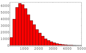
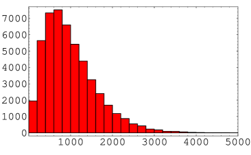
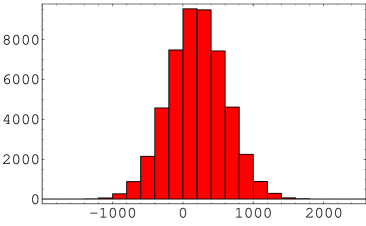
In Figure 13 we see that the distribution of DSC has a Gaussian profile with a mean different from zero, as can be understood from equations (4.22) and (4.23). We check that the found mean () and standard deviation () of this distribution are in agreement with the values expected respectively from equation (4.22) and equation (4.23), for the chosen value of (). The probability of quadrupole amplitude increasing (decreasing) is ().
9 Conclusion
We have developed an analytical model and numerical analyses to evaluate the DSC in spinning CMB anisotropy missions. Although our study is mainly devoted to the Planck project, the formalism and method are relatively general and allow to focus on the most relevant DSC implications. We quantify this systematic effect as a function of few parameters: the relative power, , entering the main spillover region with respect to the total one, the solid angle subtended by the main spillover region, the angle, , between the directions of the main spillover and the spacecraft spin axis, and, finally, a phase, , describing the displacement of the main spillover centre direction from the plane defined by the spacecraft spin axis and the telescope line of sight. The first and third of these parameters turn out to be the most relevant (at least for small , as in the case of Planck). Also, we have addressed the coupling of this effect with the observational strategy, with and without displacements of the spacecraft spin axis from the ecliptical plane. We have investigated the relevance of performing multiple surveys and the effect introduced by a possible uncompleteness (or overcompleteness) of one of the considered surveys.
The analytical approach, applied to a simple observational strategy (e.g. the NSS, in the context of Planck) and perturbatively in , has been used to focus on low multipoles, albeit some general properties have been found for odd and even . The systematic effect vanishes for an even number of complete sky surveys, except for when . We predict a contamination of the dipole itself, independently of the considered number of surveys and mainly depending on and . We have shown that when a phase is introduced, not only the dipole but also all the odd multipoles are present to linear order in . We find also that the quadrupole is affected and its observed amplitude is related to the intrinsic sky realization (). A statistical analysis has been performed aimed at the computation of the probability of increasing or decreasing of the observed quadrupole amplitude with respect the intrinsic one.
With numerical simulations, based on a dedicated updated code already applied in straylight analyses, we verify the above results and extend the analysis to different scanning strategies and significant displacements of the main spillover centre direction from the spin axis direction even for higher and uncomplete (or overcomplete) surveys. Various aspects relevant in CMB space projects (such as implications for calibration, impact on polarization measurements, accuracy requirement in the far beam knowledge for data analysis applications, scanning strategy dependence) have been discussed.
Our analysis shows that DSC should be carefully taken into account for an high precision calibration of the data from the Planck receivers and for an accurate evaluation of the quadrupole amplitude of the CMB pattern.
Acknowledgements. We warmly acknowledge all the members of the Planck Systematic Effect Working Group for many discussions and collaborations. It is a pleasure to thank M. Bersanelli, N. Mandolesi, P. Naselsky, F. Pasian, J. Tauber, and A. Zacchei for stimulating conversations. Some of the results in this paper have been derived using HEALPix (Górski et al., 2005). We wish to thank the referee for useful comments. This work has been done in the framework of the Planck LFI activities.
References
- Abramo & Sodre (2003) Abramo L.R., Sodre L.J., arXiv: astro-ph/0312124
- Barnes et al. (2003) Barnes C. et al., 2003, ApJS, 148, 51
- Bennett et al. (2003a) Bennett C.L. et al., 2003, ApJS, 148, 1
- Bennett et al. (2003b) Bennett C.L. et al., 2003, ApJS, 148, 97
- Bernard et al. (2002) Bernard J.P., Puget J.L., Sygnet J.F., Lamarre J.M., 2002, Draft note on HFI’s view on Planck Scanning Strategy, Technical Note PL-HFI-IAS-TN-SCAN01, 0.2.1
- Bersanelli et al. (1997) Bersanelli M., Muciaccia P.F., Natoli P., Vittorio N., Mandolesi N., 1997, A&AS, 121, 393
- Bouchet & Gispert (1999) Bouchet F.R. and Gispert R., 1999, NA, 4, 443
- Burigana et al. (1998) Burigana C., Maino D., Mandolesi N., Pierpaoli E., Bersanelli M., Danese L., Attolini M.R., 1998, A&AS, 130, 551
- Burigana et al. (2000) Burigana C., Natoli P., Vittorio N., Mandolesi N., Bersanelli M., 2000, Int. Rep. TeSRE/CNR 272/2000, April 2000
- Burigana et al. (2001a) Burigana C., Maino D., Gorski K.M., Mandolesi N., Bersanelli M., Villa F., Valenziano L., Wandelt B.D., Maltoni M., Hivon E., 2001, A&A, 373, 345
- Burigana et al. (2001b) Burigana C., Natoli P., Vittorio N., Mandolesi N., Bersanelli M., 2001, Experimental Astronomy, 12/2, 87
- Burigana et al. (2004) Burigana C., Sandri M., Villa F., Maino D., Paladini R., Baccigalupi C., Bersanelli M., Mandolesi N., 2004, A&A, 428, 311
- Cappellini et al. (2003) Cappellini B., Maino D., Albetti G., Platania P., Paladini R., Mennella A., Bersanelli M., 2003, A&A, 409, 375
- Copi et al. (2006) Copi C., Huterer D., Schwarz D., Starkman G., preprint arXiv: astro-ph/0605135
- De Zotti et al. (1999) De Zotti G. et al., 1999, in Proceedings of the EC-TMR Conference “3 K Cosmology”, Roma, Italy, 5-10 October 1998, AIP Conference Proc. 476, Maiani L., Melchiorri F., Vittorio N., (Eds.), 204, astro-ph/9902103
- Dupac & Tauber (2005) Dupac X., Tauber J., 2005, A&A, 430,636
- Efstathiou (2003) Efstathiou G., 2003, Mon. Not. Roy. Astron. Soc. 346 L26
- Górski et al. (2005) Górski K.M., Hivon E., Banday A.J., Wandelt B.D., Hansen F.K., Reinecke M., Bartelman M., 2005, ApJ, 622, 759
- Gruppuso, Burigana & Finelli (2004) Gruppuso A., Burigana C., Finelli F. 2004, Internal Report IASF-BO 405/2004
- Gruppuso, Burigana & Finelli (2005) Gruppuso A., Burigana C., Finelli F. 2005, Internal Report IASF-BO 416/2005
- Gruppuso, Burigana & Finelli (2006) Gruppuso A., Burigana C., Finelli F. 2006, in proc. Int. Conf. “CMB and Physics of the Early Universe”, 20-22 April 2006, Ischia, Italy, in press, astro-ph/0607413
- Harrison et al. (2006) Harrison D. et al., 2006, in proc. Int. Conf. “CMB and Physics of the Early Universe”, 20-22 April 2006, Ischia, Italy, in press
- Hinshaw et al. (1996) Hinshaw G. et al., 1996, Astrophys. J. 464 (1996) L17
- Jarosik et al. (2006) Jarosik N. et al., 2006, ApJ, submitted, astro-ph/0603452
- Lamarre et al. (2002) Lamarre J.M. et al., 2002, in “Experimental Cosmology at millimetre wavelengths – 2K1BC Workshop”, Breuil-Cervinia (AO), Valle d’Aosta, Italy, 9-13 July 2001, AIP Conference Proc. 616, De Petris M., Gervasi M., (Eds.), 213
- Maino et al. (1999) Maino D., Burigana C., Maltoni M., Wandelt B.D., Górski K.M., Malaspina M., Bersanelli M., Mandolesi N., Banday A.J., Hivon E., 1999, A&AS, 140, 383
- Mandolesi et al. (1998) Mandolesi, N. et al., 1998, Planck LFI, A proposal submitted to ESA
- Mandolesi et al. (2002) Mandolesi N. et al., 2002, in “Experimental Cosmology at millimetre wavelengths – 2K1BC Workshop”, Breuil-Cervinia (AO), Valle d’Aosta, Italy, 9-13 July 2001, AIP Conference Proc. 616, De Petris M., Gervasi M., (Eds.), 193
- Maris et al. (2006) Maris M. et al., 2006, in Memorie della SAIt, XLIX Congresso della Societ Astronomica Italiana, Catania, May 5-7, 2005, Leto G., Zuccarello F., (Eds.), in press
- Page et al. (2006) Page L. et al., 2006, ApJ, submitted, astro-ph/0603450
- Piat et al. (2002) Piat M., Lagache G., Bernard J.P., Giard M., Puget J.L., 2002, A&A, 393, 359
- Puget et al. (1998) Puget J.L. et al., 1998, HFI for the Planck Mission, A proposal submitted to ESA
- Sakurai (1985) Sakurai J.J., Modern Quantum Mechanics. Revised Edition. 1985 Addison-Wesley Publishing Company, Inc.
- Sandri et al. (2004) Sandri M., Villa F., Nesti R., Burigana C., Bersanelli M., Mandolesi N., 2004, A&A, 428, 299
- Spergel et al. (2003) Spergel D. N. et al., 2003, ApJS, 148, 175
- Spergel et al. (2006) Spergel D. N. et al., 2006, ApJ, submitted, astro-ph/0603449
- Tauber (2001) Tauber J. A., 2001, in “The Extragalactic Infrared Background and its Cosmological Implications”, Proceedings of the IAU Symposium, Vol. 204, Harwit M., (Ed.), 493
- Tauber (2006) Tauber J. A., 2006, in “The Many Scales in the Universe”, JENAM 2004 Astrophysics Reviews, Springer, Del Toro Iniesta J.C. et al., (Eds.), 35
- Tegmark, de Oliveira-Costa & Hamilton (2003) Tegmark M., de Oliveira-Costa A., Hamilton A., 2003, Phys. Rev. D 68 123523