The clustering of narrow-line AGN in the local Universe

Abstract

We have analyzed the clustering of $\sim 90,000$ narrow-line AGN drawn from the Data Release 4 (DR4) of the Sloan Digital Sky Survey. Our analysis addresses the following questions: a) How do the locations of galaxies within the large-scale distribution of dark matter influence ongoing accretion onto their central black holes? b) Is AGN activity triggered by interactions or mergers between galaxies? We compute the cross-correlation between AGN and a reference sample of galaxies drawn from the DR4. We compare this to results for control samples of inactive galaxies matched simultaneously in redshift, stellar mass, concentration, velocity dispersion and mean stellar age, as measured by the 4000 Å  break strength. We also compare near-neighbour counts around AGN and around the control galaxies. On scales larger than a few Mpc, AGN have almost the same clustering amplitude as the control sample. This demonstrates that AGN host galaxies and inactive control galaxies populate dark matter halos of similar mass. On scales between 100 kpc and 1 Mpc, AGN are clustered more weakly than the control galaxies. We use mock catalogues constructed from high-resolution N-body simulations to interpret this anti-bias, showing that the observed effect is easily understood if AGN are preferentially located at the centres of their dark matter halos. On scales less than 70 kpc, AGN cluster marginally more strongly than the control sample, but the effect is weak. When compared to the control sample, we find that only one in a hundred AGN has an extra neighbour within a radius of 70 kpc. This excess increases as a function of the accretion rate onto the black hole, but it does not rise above the few percent level. Although interactions between galaxies may be responsible for triggering nuclear activity in a minority of nearby AGN, some other mechanism is required to explain the activity seen in the majority of the objects in our sample.

1 Introduction

A major goal in the study of AGN has been to understand the physical mechanism(s) responsible for triggering accretion onto the central supermassive black hole and enhanced activity in the nucleus of the galaxy. From a theoretical standpoint, N-body simulations that treat the hydrodynamics of the gas have shown that interactions between galaxies can bring gas from the disk to the central regions of the galaxy, leading to enhanced star formation in the bulge (Barnes & Hernquist, 1992; Mihos & Hernquist, 1996). It is then natural to speculate that some of this gas will be accreted onto the central supermassive black hole and that this will trigger activity in the nucleus of the galaxy. However, there has been little clear observational evidence in support of this hypothesis.

Many observational studies have examined the correlations between AGN activity in galaxies and their local environment. These analyses have produced contradictory results. Early studies (see for example Petrosian, 1982; Dahari, 1984; Keel et al., 1985) noted that powerful Seyfert galaxies appear to show an excess of close companions relative to their non-active counterparts. More recent analyses of larger and more complete samples of Seyfert galaxies have reached the opposite conclusion (e.g. Schmitt, 2001; Miller et al., 2003). Studies of X-ray selected AGN at intermediate redshifts also find no evidence for excess near-neighbour counts or enhanced levels of galaxy asymmetry (Grogin et al., 2005; Waskett et al., 2005). On the other hand, a recent study of the local environment of a sample of $\sim 2000$ quasars at $z<0.4$ drawn from the Sloan Digital Sky Survey (Serber et al., 2006) concluded that quasars do have a significant local excess of neighbours when compared to $L_{*}$ galaxies , but only on small scales ($<0.2$ Mpc). These authors found the the excess to be significantly larger for the most luminous systems. This study suggests that the disagreement between different studies may reflect the fact that they targeted AGN with different intrinsic luminosities.

There have also been many studies of the large-scale clustering of AGN. This is usually quantified using the two-point correlation function (2PCF). In the standard model for structure formation, the amplitude of the two-point correlation function on scales larger than a few Mpc provides a direct measure of the mass of the dark matter halos that host the AGN. The large redshift surveys assembled in recent years, in particular the two-degree Field QSO Redshift Survey (2QZ; Croom et al., 2001) and the Sloan Digital Sky Survey (SDSS; York et al., 2000), have allowed the clustering of quasars to be studied with unprecedented accuracy. The cross-correlation between QSOs in the 2QZ and galaxies in the two-degree Field Galaxy Redshift Survey (2dFGRS; Colless et al., 2001), measured by Croom et al. (2005), is found to be identical to the autocorrelation of $L_{*}$ galaxies (a mean bias $b_{QG}=0.97\pm 0.05$). Measurements of the two-point correlation function of narrow-line AGN in the SDSS have been carried out by Wake et al. (2004). The results are similar to those for quasars – the amplitude of the AGN autocorrelation function is consistent with the autocorrelation function of luminous galaxies on scales from 0.2 to 100 $h^{-1}$ Mpc. Similar results are found for X-ray selected AGN (Gilli et al., 2005; Mullis et al., 2005). On the other hand, radio-loud AGN appear to be significantly more clustered on large scales (Magliocchetti et al., 1999, 2004; Overzier et al., 2003), demonstrating that they reside in massive dark matter halos. This is consistent with the fact that in the local Universe, radio-loud AGN are located in significantly more massive host galaxies than optical AGN (e.g. Best et al., 2005). Constantin & Vogeley (2006) analyzed AGN in the SDSS Data Release 2 sample and find that LINERs are more strongly clustered than Seyfert galaxies. Once again this is consistent with the fact that LINERs are found in more massive host galaxies that Seyferts (Kauffmann et al., 2003; Kewley et al., 2006).

In this paper, we analyze the clustering properties of 89,211 narrow-line AGN selected from the Data Release 4 (DR4) of the Sloan Digital Sky Survey using the procedure described in Kauffmann et al. (2003). Our methodology for computing correlation functions in the SDSS has been described in detail in Li et al. (2006), where the dependence of clustering on physical properties such as stellar mass, age of the stellar population, concentration and stellar surface mass density was studied. In this paper, we extend this analysis to AGN. Our approach differs from previous studies in the following ways:

1. We compute AGN-galaxy cross-correlations from scales of a few tens of kpc to scales of $\sim$10 Mpc. This allows us to study the detailed scale dependence of the AGN clustering amplitude.

2. We study how the clustering depends on both the black hole mass (estimated using the central velocity dispersion of the galaxy) and the accretion rate relative to the Eddington rate (estimated using L[OIII], where L[OIII] is the [OIII]$\lambda$5007 line luminosity, and $M_{BH}$ is the black hole mass estimated from the central stellar velocity dispersion of the host).

3. We wish to isolate the effect of the accreting black hole, so the clustering is always compared to the results obtained for control samples of inactive galaxies that are very closely matched to our AGN sample. We match simultaneously in redshift, mass, and structural properties and we test the effect of additionally matching the age of the stellar population as characterized by the 4000 Å break index D_n(4000).

4. We have constructed mock catalogues using the high resolution Millennium Run simulation (Springel et al., 2005). The mock catalogues match the geometry and selection function of galaxies in the DR4 large-scale structure sample and they also reproduce the luminosity and stellar mass function of SDSS galaxies, as well as the shape and amplitude of the correlation functions in different bins of luminosity and stellar mass. We use these catalogues to explore in detail how AGN trace the underlying galaxy and halo populations.

Our paper is organized as follows: In section 2, we describe the AGN and control samples that were used in the analysis. In section 3, we describe how we construct mock catalogues from the Millennium Simulation and use these to correct for effects such as fibre collisions. Section 4 describes our clustering estimator; section 5 describes the observational results and in section 6, we describe how we use our mock catalogues to extract physical information from the data. Finally in section 7, we summarize our results and present our conclusions.

2 Description of Samples

2.1 The SDSS Spectroscopic Sample

The data analyzed in this study are drawn from the Sloan Digital Sky Survey (SDSS). The survey goals are to obtain photometry of a quarter of the sky and spectra of nearly one million objects. Imaging is obtained in the u, g, r, i, z bands (Fukugita et al., 1996; Smith et al., 2002; Ivezić et al., 2004) with a special purpose drift scan camera (Gunn et al., 1998) mounted on the SDSS 2.5 meter telescope (Gunn et al., 2006) at Apache Point Observatory. The imaging data are photometrically (Hogg et al., 2001; Tucker et al., 2005) and astrometrically (Pier et al., 2003) calibrated, and used to select stars, galaxies, and quasars for follow-up fibre spectroscopy. Spectroscopic fibres are assigned to objects on the sky using an efficient tiling algorithm designed to optimize completeness (Blanton et al., 2003). The details of the survey strategy can be found in York et al. (2000) and an overview of the data pipelines and products is provided in the Early Data Release paper (Stoughton et al., 2002). More details on the photmetric pipeline can be found in Lupton et al. (2001).

Our parent sample for this study is composed of 397,344 objects which have been spectroscopically confirmed as galaxies and have data publicly available in the SDSS Data Release 4 (Adelman-McCarthy et al., 2006). These galaxies are part of the SDSS ‘main’ galaxy sample used for large scale structure studies (Strauss et al., 2002) and have Petrosian $r$ magnitudes in the range $14.5<r<17.77$ after correction for foreground galactic extinction using the reddening maps of Schlegel, Finkbeiner, & Davis (1998). Their redshift distribution extends from $\sim 0.005$ to 0.30, with a median $z$ of 0.10.

The SDSS spectra are obtained with two 320-fibre spectrographs mounted on the SDSS 2.5-meter telescope. Fibers 3 arcsec in diameter are manually plugged into custom-drilled aluminum plates mounted at the focal plane of the telescope. The spectra are exposed for 45 minutes or until a fiducial signal-to-noise (S/N) is reached. The median S/N per pixel for galaxies in the main sample is $\sim 14$. The spectra are processed by an automated pipeline, which flux and wavelength calibrates the data from 3800 to 9200 Å. The instrumental resolution is R $\equiv\lambda/\delta\lambda$ = 1850 – 2200 (FWHM$\sim 2.4$ Å at 5000 Å).

2.2 The AGN and control samples

We have performed a careful subtraction of the stellar absorption-line spectrum before measuring the nebular emission-lines. This is accomplished by fitting the emission-line-free regions of the spectrum with a model galaxy spectrum computed using the new population synthesis code of Bruzual & Charlot (2003), which incorporates a high resolution (3 Å FWHM) stellar library. A set of 39 model template spectra were used spanning a wide range in age and metallicity. After convolving the template spectra to the measured stellar velocity dispersion of an individual SDSS galaxy, the best fit to the galaxy spectrum is constructed from a non-negative linear combination of the template spectra. Further details are given in Tremonti et al. (2004). Physical parameters such as stellar masses, metallicities, and star formation rates have been estimated using the spectra and these are publically available at http://www.mpa-garching.mpg.de/SDSS/. The reader is referred to Tremonti et al. (2004) and Brinchmann et al. (2004) for more details.

AGN are selected from the subset of galaxies with $S/N>3$ in the four emission lines [OIII]$\lambda$5007, H$\beta$, [NII]$\lambda$6583, H$\alpha$. Following Kauffmann et al. (2003), a galaxy is defined to be an AGN if

$$\log([\rm{OIII}]/H\beta)>0.61/(\log([\rm{NII}]/H\alpha)-0.05)+1.3.$$ (1)

We divide all the AGN into three subsamples according to logarithmic stellar velocity dispersion $\log_{10}\sigma_{\ast}$. It is also interesting to study how clustering depends on the strength of nuclear activity in the galaxy. In order to adress this issue, we follow Heckman et al. (2004) and use the [O iii] emission line luminosity as an indicator of the rate at which matter is accreting onto the central supermassive black hole, and we use the relation given in Tremaine et al. (2002) to estimate black hole masses from the stellar velocity dispersion measured within the fibre aperture. We then use the ratio $L$[O iii]/M_BH as a measure of the accretion rate relative to the Eddington rate, to define subsamples of “powerful” and ”weak” AGN. (Note that in the current analysis, L[OIII] is corrected for dust extinction.) The AGN in each $\log_{10}\sigma_{\ast}$ subsample are ordered by decreasing $L$[O iii]/M_BH. The top 25% are defined as “powerful” and the bottom 25% are “weak”. For each AGN sample, we construct 20 control samples of non-AGN by simultaneously matching four physical parameters: redshift, stellar mass, concentration and stellar velocity dispersion. We have also constructed control samples where the 4000 Å break strength is matched in addition to these parameters. The matching tolerances are $\Delta cz<500$ km s^-1, $\Delta\log M_{*}<0.1$, $\Delta\sigma_{*}<20$ km s^-1 , $\Delta C<0.1$ and $\Delta$D_n(4000)$<0.05$.

We correct the [OIII] luminosities of the AGN in our sample for dust using the difference between the observed H$\alpha$/H$\beta$ emission line flux ratios and the case-B recombination value (2.86). We assumed an attenuation law of the form $\tau_{\lambda}\propto\lambda^{-0.7}$ (Charlot & Fall, 2000) This procedure has clear physical meaning in the “pure” Seyfert 2’s and LINERs. In the case of the transition objects, the lines will arise both in the NLR and the surrounding HII regions, with a greater relative AGN contribution to [OIII] than to the Balmer lines. Thus, a dust correction to [OIII] based on the ratio H$\alpha$/H$\beta$ should be regarded as at best approximate.

2.3 Reference galaxy sample

We use the New York University Value Added Galaxy Catalogue (NYU-VAGC) to construct a reference sample of galaxies, which are cross-correlated with the AGN sample. The original NYU-VAGC is a catalogue of local galaxies (mostly below $z\approx 0.3$) constructed by Blanton et al. (2005) based on the SDSS DR2. Here we use a new version of the NYU-VAGC (Sample dr4), which is based on SDSS DR4. The NYU-VAGC is described in detail in Blanton et al. (2005).

We have constructed two reference samples: 1) a spectroscopic reference sample , which is used to compute the projected AGN-galaxy cross-correlation function $w(r_{p})$; 2) a photometric reference sample, which is used to calculate counts of close neighbours around AGN

The spectroscopic reference sample is constructed by selecting from Sample dr4 all galaxies with $14.5<r<17.6$ that are identified as galaxies from the Main sample (note that $r$-band magnitude has been corrected for foreground extinction). The galaxies are also restricted to the redshift range $0.01\leq z\leq 0.3$, and the absolute magnitude range $-23<M_{{}^{0.1}r}<-17$. The spectroscopic reference sample contains 292,782 galaxies. We do not consider galaxies fainter than $M_{{}^{0.1}r}=-17$, because the volume covered by such faint samples is very small and the results are subject to large errors as a result of cosmic variance (see for example Fig. 6 of Li et al., 2006). The faint apparent magnitude limit of 17.6 is chosen to yield uniform galaxy sample that is complete over the entire area of the survey.

The photometric reference sample is also constructed from Sample dr4 by selecting all galaxies with $14.5<r<19$. The resulting sample includes 1,065,183 galaxies. Throughout this work we adopt standard $\lambda$CDM cosmological parameters: $\Omega=0.3$, $\Omega_{\Lambda}=0.7$, and H₀ = 70 km s^-1 Mpc^-1.

3 Mock Catalogues

In this section we describe how we construct a large set of mock galaxy samples with the same geometry and selection function as the spectroscopic samples described in the previous section . We will use these mock catalogues to test our method for correcting for the effect of fibre collisions on the measurement of the AGN-galaxy cross-correlation function on small scales. We will also use these mock catalogues to construct models of AGN clustering for comparison with the observations.

3.1 Galaxy properties in the Millennium Simulation

Our mock catalogues are constructed using the Millennium Simulation (Springel et al., 2005), a very large simulation of the concordance $\Lambda$CDM cosmogony with $10^{10}$ particles. The chosen simulation volume is a periodic box of size $L_{box}=500h^{-1}$ Mpc on a side, which implies a particle mass of $8.6\times 10^{8}$ 4$h^{-1}M_{\odot}$. Haloes and subhaloes at all output snapshots are identified using the subfind algorithm described in Springel et al. (2001) and merger trees are then constructed that describe how haloes grow as the Universe evolves. Croton et al. (2006) implemented a model of the baryonic physics in these simulations in order to simulate the formation and evolution of galaxies and their central supermassive black holes (see Croton et al., 2006, for more details). This model produced a catalogue of 9 million galaxies at $z=0$ down to a limiting absolute magnitude limit of $M_{r}-5\log h=-16.6$. This catalogue is well-matched to many properties of the present-day galaxy population (luminosity-colour distributions, clustering etc.). It is publically available at http://www.mpa-garching.mpg.de/galform/agnpaper. In our work, we adopt the positions and velocities of the galaxies given in the Croton et al. catalogue. The $r$-band luminosities and stellar masses are assigned to each model galaxy, using the parametrized functions described by Wang et al. (2006). These functions relate the physical properties of galaxies to the quantity $M_{infall}$, defined as the mass of the halo at the epoch when the galaxy was last the central dominant object in its own halo. They were chosen so as to give close fits to the results of the physical galaxy formation model of Croton et al. (2006), but their coefficients were adjusted to improve the fit to the SDSS data, in particular the galaxy mass function at the low mass end. Extensive tests have shown that the adopted parametrized relations allow us to accurately match the luminosity and stellar mass functions of galaxies in the SDSS, as well as the shape and amplitude of the two point correlation function of galaxies in different luminosity and stellar mass ranges (Li et al., 2006; Wang et al., 2006).

3.2 Constructing the catalogues

Our aim is to construct mock galaxy redshift surveys that have the same geometry and selection function as the SDSS DR4. A detailed account of the observational selection effects accompanies the NYU-VAGC release. The survey geometry is expressed as a set of disjoint convex spherical polygons, defined by a set of “caps”. This methodology was developed by Andrew Hamilton to deal accurately and efficiently with the complex angular masks of galaxy surveys (Hamilton & Tegmark, 2002) . The advantage of using this method is that it is easy to determine whether a point is inside or outside a given polygon (Tegmark et al., 2002). The redshift sampling completeness is then defined as the number of galaxies with redshifts divided by the total number of spectroscopic targets in the polygon. The completeness is thus a dimensionless number between 0 and 1, and it is constant within each of the polygons. The limiting magnitude in each polygon is also provided (it changes slightly across the survey region).

We construct our mock catalogues using the methods described in Yang et al. (2004), except that we position the virtual observer randomly inside the simulation and not at the centre of the box. Because the survey extends out to $z\sim 0.3$, this implies that we need to cover a volume that extends to a depth of $900h^{-1}$ Mpc, i.e. twice that of the Millennium catalogue. We thus create $5\times 5\times 5$ periodic replications of the simulation box and place the observer randomly within the central box, so that the required depth can be achieved in all directions for the observer.

We produce 20 mock catalogues by following the procedure described below:

1. We randomly place a virtual observer in the stack of boxes described above. We define a ($\alpha$,$\delta$)-coordinate frame and remove all galaxies that lie outside the survey region.

2. For each galaxy we compute the redshift as ”seen” by the virtual observer. The redshift is determined by the comoving distance and the peculiar velocity of the galaxy.

3. We compute the $r$-band apparent magnitude of each galaxy from its absolute magnitude $M_{r}$ and its redshift, applying a (negative) K-correction but neglecting any evolutionary correction. We then select galaxies according to the position-dependent magnitude limit (provided in the Sample dr4) and apply a (positive) K-correction to compute $M_{{}^{0.1}r}$, the $r$-band absolute magnitude of the galaxy at $z=0.1$.

4. To mimic the position-dependent completeness, we randomly eliminate galaxies using the completeness masks provided in Sample dr4.

5. Finally, we mimic the actual selection criteria of our own reference sample by restricting galaxies in the mock catalogue to $0.01<z<0.3$, $14.5<r<17.6$ and $-23<M_{{}^{0.1}r}<-17$.

Figure 1 shows the equatorial distribution of galaxies in one of our mock catalogues, compared to that in the observational sample. The average number of galaxies in our mock catalogues is $\sim$320,000, with a r.m.s. dispersion of $\sim 9000$, in good agreement with the observed number.

Figure 1: Equatorial distribution of right ascension and redshift for galaxies within 6^∘ of the equator in the SDSS (left) and in one of our mock catalogues (right).

3.3 Fibre collisions

The procedure described above does not account for the fact that the spectroscopic target selection becomes increasingly incomplete in regions of the sky where the galaxy density is high, because two fibres cannot be positioned closer than 55 arcseconds from each other. In order to mimic these fibre “collisions”, we modify step (4) above. We no longer randomly sample galaxies using the completeness masks. Instead, we assign fibres to our mock galaxies using a procedure that is designed to mimic the tiling code that assigns spectroscopic fibres to SDSS target galaxies (Blanton et al., 2003). We run a friends-of-friends grouping algorithm on the mock galaxies with a 55^′′ linking length. Isolated galaxies, i.e. those in single-member groups, are are always assigned fibres. If two targets collide, we simply pick one at random to be the spectroscopically targeted galaxy. For groups with more than two members, we need to determine which members will be assigned fibres and which will not. The resulting groups are almost always of sufficiently low multiplicity so that in principle, one could simply check all possibilities to find the best possible combination of galaxies that would eliminate fibre collisions (this is the procedure adopted in the SDSS target selection). In our work we use a somewhat more efficient method. For each group, we calculate the geometric centre. The group members located closer to the center are preferentially eliminated. For example, in a triple collision this algorithm will keep the outer two members rather than the middle one.

This procedure is complicated by the fact that some fraction of the sky will be covered with overlaps of different tiles (Each spectroscopic fibre plug plate is referred as a “tile”, which has a circular field of view with a radius of $1^{\circ}_{.}49$.). About 30 % of the sky is covered in such overlaps. This means that if, for example, a binary group covered by two ore more tiles, both of the group members can be assigned fibres. We take this into account by iteratively repeating the procedure described above, as follows.

1. First, we determine the number of tiles that cover a given galaxy and set the quantity $n_{chances}$ equal to this number. For example, $n_{chances}=2$ for a galaxy covered by two tiles; this galaxy has two chances to be assigned a fibre.

2. We assign fibres by applying the algorithm described above to those galaxies with $n_{chances}>0$. If a galaxy obtains a fibre in this procedure, then the quantity $n_{chances}$ is set to zero. If not, we set $n_{chances}=n_{chances}-1$.

3. Step (ii) is repeated until $n_{chances}$ reaches zero for all galaxies. All galaxies that are not assigned fibres are then removed from our mock catalogue.

4. Finally, we remove a number of galaxies at random so that the resulting mock sample has the same overall position-dependent completeness as the real SDSS sample.

4 Clustering measures

In order to compute the two-point cross-correlation function (2PCF) $\xi(r_{p},\pi)$ between the AGN host (or matched control) sample and the reference galaxy sample , we have constructed random samples that are designed to include all observational selection effects. This is described in detail in Li et al. (2006). $\xi(r_{p},\pi)$ is then calculated using the estimator

$$\xi(r_{p},\pi)=\frac{N_{R}}{N_{D}}\frac{QD(r_{p},\pi)}{QR(r_{p},\pi)}-1,$$ (2)

where $r_{p}$ and $\pi$ are the separations perpendicular and parallel to the line of sight; $N_{D}$ and $N_{R}$ are the number of galaxies in the reference sample and in the random sample; $QD(r_{p},\pi)$ and $QR(r_{p},\pi)$ are the cross pair counts between AGN (or control) and the reference sample, and between AGN (or control) and the random sample, respectively.

In what follows, we focus on the projection of $\xi(r_{p},\pi)$ along the line of sight:

$$w_{p}(r_{p})=\int_{-\infty}^{+\infty}\xi(r_{p},\pi)d\pi=\sum_{i}\xi(r_{p},\pi_{i})\Delta\pi_{i}.$$ (3)

Here the summation for computing $w_{p}(r_{p})$ runs from $\pi_{1}=-39.5$ h^-1 Mpc to $\pi_{80}=39.5$ h^-1 Mpc, with $\Delta\pi_{i}=1$ h^-1 Mpc.

The errors on the clustering measurements are estimated using the bootstrap resampling technique (Barrow, Bhavsar, & Sonoda, 1984). We generate 100 bootstrap samples from the observations and compute the correlation functions for each sample using the weighting scheme (but not the approximate formula) given by Mo, Jing, & Boerner (1992). The errors are then given by the scatter of the measurements among these bootstrap samples. More details about our procedures and tests of our methodology can be found in Li et al. (2006). We also obtain robust estimates of our uncertainties from the scatter between the results obtained from disjoint areas of the sky.

We are particularly interested in the amplitude of the AGN-reference galaxy cross-correlation on small scales ($<100$ kpc), because this allows us to evaluate whether mergers and interactions play a role in triggering AGN activity. A careful correction for the effect of fibre collisions when measuring the clustering is thus very important. As described in Li et al. (2006), we correct for fibre collisions by comparing the angular 2PCF of the spectroscopic sample with that of the parent photometric sample. Here we use our mock SDSS catalogues to test the correction method. We calculate the angular correlation functions $w_{z}(\theta)$ and $w_{p}(\theta)$ using mock catalogues with and without fibre collisions. The function

$$F(\theta)=\frac{1+w_{z}(\theta)}{1+w_{p}(\theta)}$$ (4)

is then used to correct for collisions by weighting each pair by $1/F(\theta)$. Figure 2 (the top panel) shows measurements of $w_{p}(r_{p})$ for galaxies in one of our mock catalogues. The solid line is the “true” correlation function calculated for the mock catalogues that do not include fibre collisions. Circles show the results when fibre collisions are included. Triangles show the results that are obtained when the 2PCF is corrected for the effect of fibre collisions using the method described above. In the bottom panel, we plot the ratios of the uncorrected and the corrected $w_{p}(r_{p})$ relative to the ”true” correlation function. As can be seen, our correction procedure works well. The turnover in the amplitude on small physical scales resulting from the lower sampling of galaxies in dense regions disappears and the corrected $w_{p}(r_{p})$ is very close to the real one. It is noticeable that there is still a very small deficit in the corrected $w_{p}(r_{p})$ on scales between 0.05 and 1 Mpc. This should not be a significant contribution to the bias between AGN and normal galaxies (see below), because fibre collisions are expected to affect the AGN and the reference galaxies in the same way.

Figure 2: Top: Projected 2PCF $w_{p}(r_{p})$ measured for the mock catalogue without including fibre collisions (solid line) and for the mock catalogue with fibre collisions (circles). The filled triangles show the measured $w_{p}(r_{p})$ for the mock after correcting the effect of fibre collisions using the method described in the text. Bottom: The ratios of the uncorrected and the corrected $w_{p}(r_{p})$ relative to the ”true” $w_{p}(r_{p})$.

5 Observational results

5.1 AGN Bias

We first compute $w_{p}^{\rm AGN/ref}(r_{p})$, the cross-correlation of the AGN sample with respect to the reference sample. As described in section 2, we have constructed two sets of 20 control samples. The first set is constructed by simultaneously matching redshift, stellar mass, concentration and stellar velocity dispersion, and the second set by additionally matching the 4000Å  break strength. We then compute $\bar{w}_{p}^{\rm contr/ref}(r_{p})$, the average cross-correlation of the control samples with respect to the reference sample. The quantity $w_{p}^{\rm AGN/ref}(r_{p})/\bar{w}_{p}^{\rm contr/ref}(r_{p})$ then measures the bias of the AGN sample with respect to the control sample of non-AGN as a function of projected radius $r_{p}$.

The results are shown in Fig. 3. In the top panel, we plot $w_{p}^{\rm AGN/ref}(r_{p})$ as circles. $\bar{w}_{p}^{\rm contr/ref}(r_{p})$ is evaluated for the two sets of control samples and the results are plotted as squares for the first set and triangles for the second set. The measurement errors are estimated using the bootstrap resampling technique described in the previous section. In the bottom panel, we plot the ratio $w_{p}^{\rm AGN/ref}(r_{p})/\bar{w}_{p}^{\rm contr/ref}(r_{p})$ for the two control samples, The errors are estimated in the same manner as in the top panel. For clarity, squares and triangles in both panels have been slightly shifted along the $r_{p}$-axis.

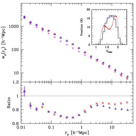
Figure 3: Top: projected cross-correlation function $w_{p}^{\rm AGN/ref}(r_{p})$ between AGN and reference galaxies is plotted as circles. The average cross-correlation between two sets of 20 control samples of non-AGN and the same reference galaxies is plotted as squares and triangles (squares: redshift, stellar mass, stellar velocity dispersion and concentration are matched; triangles: the control samples are constructed by additionally matching the 4000Å-break strength). The inset compares the D₄₀₀₀ distribution for the two sets of control samples, with red for the former set and blue for the latter. The histogram shows the D_n(4000) distribution for the AGN. Bottom: ratio of the $w_{p}(r_{p})$ measurement of AGN to that of non-AGN. Symbols are the same as in the top panel.

Figure 3 shows that there exists a scale-dependent bias in the distribution of AGN relative to that of normal galaxies. In particular, the ratio between the two cross-correlations appears to exhibit a pronounced “dip” at scales between 100 kpc and 1 Mpc. We note that errorbars estimated using the bootstrap resampling technique do not take into account effects due to cosmic variance. The coherence length of the large scale structure is large and even in a survey as big as the SDSS, this can induce significant fluctuations in the amplitude of the correlation function from one part of the sky to another. The difference in the clustering amplitude of AGN and non-AGN shown in Figure 3 is only a 10-30% effect , so it is important to test whether the dip seen in Figure 3 is truly robust.

We have thus divided the survey into 6 different areas on the sky. Each subsample includes $\sim 12,000$ AGN. We recompute the AGN bias for each of these subsamples and the results are shown in Fig. 4. Note that in this plot, we only use a single control sample to compute the bias, not the average of 20 control samples as in Figure 3. The scatter between the different curves in Figure 4 thus provides an upper limit to the true error in the measurement of the bias. As can be seen, on small scales ($<$ 50 kpc) , the different subsamples scatter in bias above and below unity. On scales between 0.1 and 1 Mpc, however, all 6 subsamples lie systematically below this line. On scales larger than 1-2 Mpc, five out of six subsamples show bias values below unity, but the effect is clearly less significant than on scales between 0.1 and 1 Mpc. In Fig. 5, we examine the dispersion in the bias measurement for the AGN sample as a whole caused by differences between the control samples. As can be seen, the scatter in the measurement of the bias between different control samples is considerably smaller than the scatter between different survey regions, showing that that cosmic variance is, in fact, the dominant source of uncertainty in our results. Once again, there is clear indication that AGN are antibiased relative to the control galaxies on scales larger than 100 kpc.

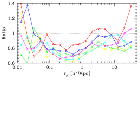
Figure 4: Ratio of the $w_{p}(r_{p})$ measurement of AGN to that of non-AGN for six disjoint regions of the survey.

We conclude that on scales between 0.1 and 1 Mpc, AGN are significantly anti-biased relative to non-AGN of the same stellar mass, concentration and stellar velocity dispersion. Figure 3 shows that this anti-bias persists even when the mean age of the stellar population is matched in addition to stellar mass and structural parameters. We note that these scales are comparable to the diameters of the dark matter halos that are expected to host galaxies with stellar masses comparable to the objects in our sample. In section 6, we construct halo occupation (HOD) models using mock catalogues constructed from the Millennium Simulation that can explain the anti-bias on these scales. As we will show, the same models naturally predict a smaller, but significant antibias on scales larger than 1 Mpc.

5.2 Dependence on black hole mass and AGN power

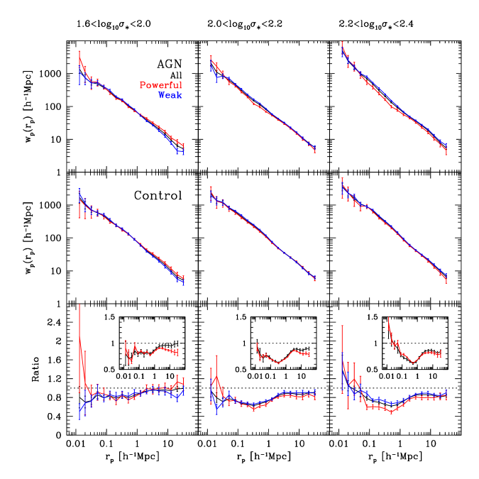
Figure 5: Top: projected cross-correlation $w_{p}(r_{p})$ in different $\sigma_{\ast}$ bins (indicated above each panel), for all AGN (black), powerful (red) and weak (blue) AGN. The powerful (weak) AGN are defined as the top (bottom) 25 per cent objects ordered by decreasing $L$[O iii]$/M_{\bullet}$. The middle row is for control samples of non-AGN and the bottom row shows the ratio between the results for the AGN and the control samples. The insets in the bottom panels compare results for all AGN using different control samples. Black is for control samples constructed by matching redshift, stellar mass, stellar velocity dispersion and concentration, while red is for control samples where the 4000Åbreak strength is also matched.

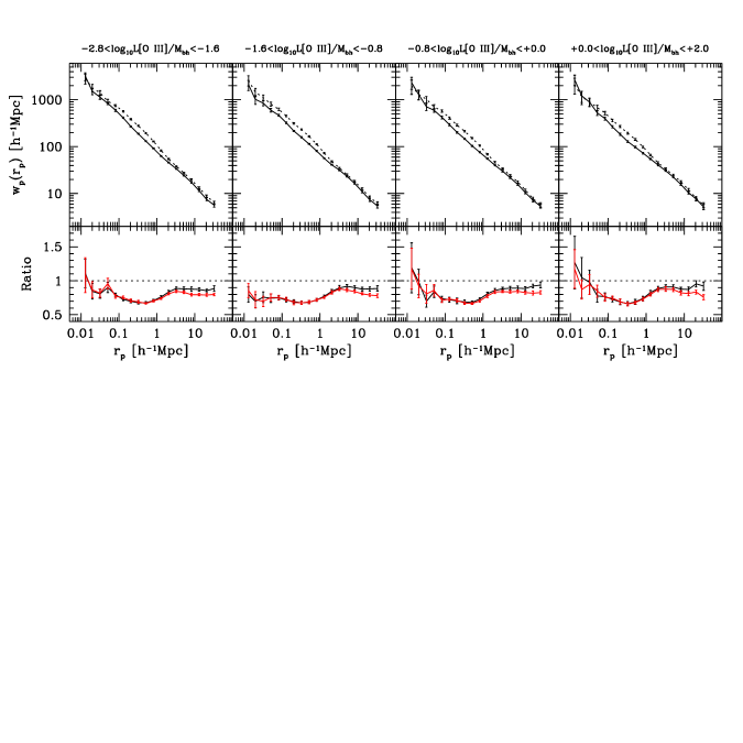
Figure 6: $w_{p}(r_{p})$ in different $L$[L iii]$/M_{\bullet}$ bins (indicated above each panel), for all AGN (solid) and for control samples of non-AGN (dashed). The small panels give the ratio between the above two (black). The red lines are results where the 4000Å-break strength is also matched when constructing control samples.

It is interesting to study how AGN clustering depends on black hole mass and the strength of nuclear activity in the galaxy. As described above, we use the stellar velocity dispersion as an indicator of the black hole mass and divide all AGN into three subsamples according to $\log_{10}\sigma_{\ast}$. We then use the ratio $L$[O iii]/M_BH as a measure of the accretion rate relative to the Eddington rate. We rank order all the AGN in a given interval of stellar velocity dispersion according to $L$[O iii]/M_BH and we define subsamples of “powerful” and ”weak” AGN as those contained within the upper and lower 25th percentiles of the distribution of this quantity.

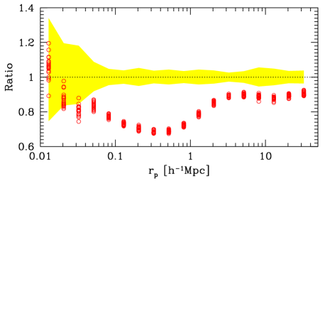
Figure 7: Ratio of the $w_{p}(r_{p})$ measurement of AGN to that of non-AGN for 20 different non-AGN control samples. The yellow shaded region shows the ratio of the $w_{p}(r_{p})$ measurements of the different non-AGN control samples relative to each other.

The results are shown in Figure 6. Panels from left to right correspond to different intervals of $\log_{10}\sigma_{\ast}$, as indicated at the top of the figure. The first two rows show the $w_{p}(r_{p})$ measurements for the AGN and the corresponding control samples. The third row shows the ratio between the two. Red (blue) lines correspond to the powerful (weak) subsamples. Black lines show results for the sample as a whole.

As mentioned previously, there are two sets of control samples: sample 1 is constructed by simultaneously matching redshift, stellar mass, concentration and stellar velocity dispersion; sample 2 is constructed by additionally matching the 4000Å break strength. For clarity, the main panels in in Figure 6 show the results only for sample 1. The insets in the bottom row compare the ratio $w_{p}^{\rm AGN/ref}(r_{p})/\bar{w}_{p}^{\rm contr/ref}(r_{p})$ for the two control samples (black corresponds to set 1 and red to set 2). The two different control samples give very similar results on scales less than a few Mpc, but the large-scale antibias is more pronounced for sample 2 (note that this is also seen in Figure 2).

As can be seen, the “dip” in clustering on scales between 0.1 and 1 Mpc is most pronounced for AGN with the largest central stellar velocity dispersions and the highest accretion rates. On scales smaller than 0.1 Mpc, more powerful AGN appear be somewhat more strongly clustered than weaker AGN and more strongly clustered than galaxies in the control sample. The error bars on the measurements are large, however, and effect is not of high significance. In Figure 7 we plot results for AGN of all velocity dispersions, but now in four different intervals of $L$[O iii]/M_BH, as indicated at the top of the figure. Once again we see a marginal tendency for AGN with higher values of $L$[O iii]/M_BH to be more strongly clustered on small scales.

5.3 Close Neighbour Counts

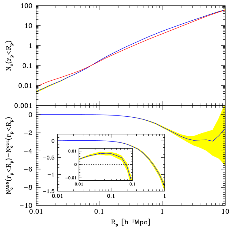
Figure 8: Top: Average counts of galaxies in the photometric sample ($r_{lim}<19$) within a given projected radius $R_{p}$ from the AGN (red) and from the control galaxies (blue). Bottom: The difference between the counts around the AGN and the control galaxies is plotted as a function of $R_{p}$. The yellow bands indicate the variance in the results between the 20 different control samples.

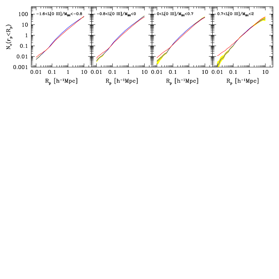
Figure 9: Same as the top panel of Fig. 8, but for four subsamples of AGN with different $L$[O iii]$/M_{\bullet}$, as indicated in each panel.

As we have discussed, one of the problems with computing the galaxy-AGN cross- correlation function on very small physical scales in the SDSS is that corrections for the effect of fibre collisions are required. These corrections are statistical in nature and even if they are correct on average, they may still introduce systematic effects in our analysis. An alternative approach is to count the number of galaxies in the vicinity of AGN in the photometric sample, which is not affected by incompleteness. The disadvantage of using the photometic sample is that many of the close neighbours will not be truly nearby systems, but rather chance projections of foreground and background galaxies that lie along the line-of-sight. We can make a statistical correction for this by evaluating the counts around randomly placed “galaxies” with the same assumed joint distribution of apparent magnitude and redshift as the AGN (control) samples.

In the upper panel of Figure 8 we plot the average correlated neighbour count (i.e. after statistical correction for uncorrelated projected neighbours) within a given value of the projected radius $R_{p}$ for the AGN sample (red) and the control samples (blue). The lower panel and its insets show the difference betweeen the average correlated counts for the AGN and control samples as a function of $R_{p}$. The variance in the counts around the control galaxies estimated from the 20 different control samples is shown in yellow. The AGN sample has a $r$-band limiting magnitude of 17.6 and the photomteric reference sample that we use is limited at $r$=19.0. In order to ensure that we are counting similar neighbours at all redshifts, the counts only include those galaxies with $r<r_{\rm AGN}+1.4$ mag. In this analysis, the control sample is matched in $r$-band apparent magnitude as well as redshift, stellar mass, velocity dispersion and concentration. This ensures that we are counting galaxies to the same limiting magnitude around both the AGN and the control galaxies.

Figure 8 shows that the counts around the AGN and the control galaxies match well on large scales. On small scales, there is a small but significant excess in the number of neighbours around AGN out to scales of $\sim 70$ kpc. As may be seen from the bottom panel of Figure 8, AGN are appromimately twice as likely to have a near neighbour as galaxies in the control sample. This does not mean, however, that every AGN has a close companion. Figure 8 also shows that only one in a hundred AGN has an additional close ($R_{p}<70$ kpc) neighbour as compared to the control galaxies. On scales larger than 100 kpc, the pair counts around the AGN dip below the counts around the control samples, leading to the “anti-bias” discussed in the previous section. This may be compensated on scales larger than several Mpc, although such compensation is not required with our present statistics.

Figure 9 shows the counts around AGN in four different ranges of L[OIII]/$M_{BH}$. As can be seen, the excess on small scales increases as a function of the accretion rate onto the black hole. However, the excess affects only a few percent of the AGN, even for the objects in our highest L[OIII]/M_BH bin. We note that Serber et al. (2006) analyzed galaxy counts around quasars compared to $L_{*}$ galaxies at the same redshift and found a clear excess on scales less than 100 kpc, very similar to the $\sim 70$ kpc scales where we see the upturn in the counts around our sample of narrow-line AGN. Serber et al also found that the excess was largest for the most luminous quasars; the excess count reached values $\sim 1$ (i.e. significantly larger than the excess found for the most powerful narrow-line AGN in our sample) for quasars with $i$-band magnitudes brighter than $-24$. If we use the relation between [OIII] line luminosity and quasar continuum luminosity of Zakamska et al. (2003) to compare the AGN in our sample to the quasars studied by Serber et al, we find that the luminosities where quasars begin to exhibit a significant excess count lie just beyond those of the AGN that populate our highest L[OIII]/M_BH bin.

Our conclusion, therefore, is that we do not find strong evidence that interactions and mergers are playing a significant role in triggering the activity in typical AGN in the local Universe. One caveat that should be mentioned is that if the activity is triggered after the merger has already taken place, our pair count statistics would not be a good diagnostic. In order to assess this, more work is needed to assess whether AGN exhibit any evidence for disturbed morphologies or stuctural peculiarities.

6 Interpretion of AGN Clustering using Halo Occupation Models

In the previous section we showed that the main difference in the AGN-galaxy cross-correlation function with respect to that of a closely matched control sample of non-AGN is that AGN are more weakly clustered on scales between 100 kpc and 1 Mpc. On larger scales, there is a much smaller difference in the clustering signal of AGN and non-AGN. The clustering amplitude of AGN on large scales provides a measure of the mass of the dark matter halos that host these objects. The fact that there is only a small difference between the AGN and the control sample tells us that AGN are found in roughly similar dark matter halos to non-AGN with the same stellar masses and structural properties.

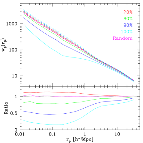
Figure 10: Top: The AGN/reference cross-correlation function calculated from the mock catalogues is plotted as solid curves, while the control/reference cross-correlations are plotted as dashed curves. The different colours indicate models in which a given percentage (as indicated on the plot) of the AGN are located at the centers of their own dark matter halos. Bottom: The ratio between the AGN/reference galaxy cross-correlation functions and the control galaxy/ reference galaxy correlation functions are plotted for the same set of models.

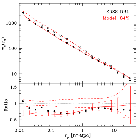
Figure 11: Top: The AGN/reference cross-correlation function calculated from the SDSS is plotted as solid circles. The open circles show the control galaxy/reference galaxy cross-correlation function from the SDSS. Results for AGN and control galaxies for our best-fit model are plotted as solid and dashed red lines. Bottom: Solid circles show the ratio $w^{\rm AGN/ref}(r_{p})/w^{\rm control/ref}(r_{p})$ for the SDSS sample. The solid red curve shows the result for our best-fit models. The error bars indicate the uncertainty due to cosmic variance as estimated from 20 different mock catalogues (see text for more details). The dashed red curves indicate the variance between different control samples from different mock catalogues (see text).

The physical scales of 0.1-1 Mpc where we do see strong differences in the clustering of AGN and non-AGN are similar to the virial diameters of the dark matter halos that are expected to host galaxies with luminosities of $\sim L_{*}$ (Mandelbaum et al., 2006). The simplest interpretation of the AGN anti-bias on these scales, therefore, is that AGN occupy preferred positions within their dark matter halos where conditions are more favourable for continued fuelling of the central black hole. One obvious preferred location would be the halo centre where gas is expected to be able to reach high enough overdensities to cool via radiative processes. In the main body of the more massive dark matter halos, most of the surrounding gas will have been shock heated to the virial temperature of the halo and will no longer be able to cool efficiently. In addition, the vast majority of galaxy-galaxy mergers within a halo will occur with the galaxy that is located at the halo centre (Springel et al., 2001).

In this section, we use our mock catalogues to test whether a model in which AGN are preferentially located at the centres of dark matter halos can fit our observational results. As mentioned in section 2, we have used the methodology introduced by Wang et al. (2006) to assign stellar masses to the galaxies in the catalogues. These authors adopted parametrized functions to relate galaxy properties such as stellar mass to the quantity $M_{infall}$, defined as the mass of the halo at the epoch where the galaxy was last the central dominant object in its own halo. It was demonstrated that these parametrized relations were able to provide an excellent fit to the basic statistical properties of galaxies in the SDSS, including the stellar mass function and the shape and amplitude of the two-point correlation function function evaluated in different stellar mass ranges. We now introduce a simple model in which $p_{AGN}$, the probability of a galaxy to be an AGN depends only on whether it is the central galaxy of its own halo.

In order to create mock AGN and control catalogues that we can compare directly with the observational data, we follow the following procedure. For every AGN in our sample, we select galaxies from the mock catalogue that have the same stellar mass and the same redshift. We then choose an AGN from among these galaxies based on whether they are central or satellite systems. The control galaxies are selected at random from the same set. The AGN and control samples are then cross-correlated with a reference sample that is drawn from the mock catalogue in exactly the same way as our real SDSS reference sample. The top panel in Figure 10 shows how the AGN/reference galaxy cross-correlation function changes as a function of the fraction of AGN that are central galaxies. Note that if the probability of being an AGN is independent of whether the galaxy is a central or a satellite system, 73% of the AGN will be central galaxies. The bottom panel of Figure 10 shows how the ratio between the AGN and control galaxy cross-correlation functions varies as this fraction changes.

As the fraction of centrally-located AGN increases, the “dip” on scales smaller than 1 Mpc becomes more and more pronounced. There is also a small decrease of the ratio $w^{\rm AGN/ref}(r_{p})/w^{\rm control/ref}(r_{p})$ on large scales. The latter effect arises because, as more and more AGN are required to be central galaxies in their own halos, they also shift into lower mass halos. High mass halos are less abundant than low mass halos and by definition, each halo can only contain one central galaxy. As the central galaxy criterion on AGN becomes more stringent, fewer AGN will reside in halos of $10^{14}-10^{15}M_{\odot}$ and more in halos with $10^{12}-10^{13}M_{\odot}$. The biggest effect, however, the dip on scales less than 1 Mpc, results from the fact that central galaxies in lower mass halos have fewer neighbours than non-central galaxies within rich groups.

In Figure 11, we compare the results of our simple model with the observational data. In the top panel, the solid and open circles show the cross-correlation functions of the AGN and the control samples respectively. The solid and dashed lines show our best-fit models, in which 84% of all AGN are located at the centres of their own dark matter halos. In the bottom panel we compare the ratio of $w(r_{p})$ for the observed AGN and control galaxies with that obtained for the model. The error bars plotted on the model curve provide an estimate of the uncertainty in the result due to cosmic variance effects. In order to estimate these errors, we have created 20 different mock catalogues by repositioning the virtual observer at random within the simulation volume. For each mock catalogue, we repeat our computations of the AGN and control galaxy cross-correlation functions. The error bars are then calculated by looking at the variance in the ratio $w^{\rm AGN/ref}(r_{p})/w^{\rm control/ref}(r_{p})$ for AGN and control galaxies selected from different catalogues. The errors estimated in this way are similar in size to the errors estimated by calculating the variance in $w^{\rm control/ref}(r_{p})$ from different mock catalogues; these errors are indicated by the dashed red lines in Figure 11. As can be seen, the model provides a good fit to the observations from scales of $\sim 30$ kpc out to scales beyond 10 Mpc. On scales smaller than 30 kpc, the AGN show a small, but significant excess in clustering with respect to the model. This is nicely in line with the results presented in the previous section.

7 Summary and Conclusions

In this paper, we have analyzed the clustering of Type 2 narrow-line AGN in the local Universe using data from the Sloan Digital Sky Survey. The two physical questions we wish to address are, a) How do the locations of galaxies within the large-scale distribution of dark matter influence ongoing accretion onto their central black holes? b)Is AGN activity triggered by interactions and mergers between galaxies? To answer these questions, we analyze the scale-dependence of the AGN/galaxy cross-correlation function relative to control samples of non-AGN that are closely matched in stellar mass, redshift, structural properties, and mean stellar age as measured by the 4000 Å  break strength. This close matching is important because previous work has established that the clustering of galaxies depends strongly on properties such as luminosity, stellar mass, colour, spectral type, mean stellar age, concentration and stellar surface mass density (Norberg et al., 2002; Zehavi et al., 2002, 2005; Li et al., 2006). Previous work has also established that AGN are not a random subsample of the the underlying galaxy population. Rather, they are found in massive, bulge-dominated galaxies; powerful AGN tend to occur in galaxies with smaller black holes and younger-than-average stellar populations for their mass (Kauffmann et al., 2003; Heckman et al., 2004). If we wish to understand whether there is a real physical connection between the location of a galaxy and the accretion state of its central black hole, it is important that we normalize out these zero’th order trends with galaxy mass, structure and mean stellar age.

When we compare the clustering of AGN relative to carefully matched control samples, and we take the errors due to cosmic variance into account, we obtain the following results:

1. On scales larger than a few Mpc, the clustering amplitude of AGN hosts does not differ significantly from that of similar but inactive galaxies.

2. On scales between 100 kpc and 1 Mpc, AGN hosts are clustered more weakly than control samples of similar but inactive galaxies.

3. On scales less than 70 kpc, AGN cluster more strongly than inactive galaxies, but the effect is weak. The excess number of close companions is only one per hundred AGN.

Our clustering results on large scales demonstrate that the host galaxies of AGN are found in similar dark matter halos to inactive galaxies with the same structural properties and stellar masses. We have used mock catalogues constructed from high-resolution N-body simulations to show that the AGN anti-bias on scales between 0.1 and 1 Mpc can be explained by AGN residing preferentially at the centres of their dark matter halos. Our result on small scales indicates that although interactions may be responsible for triggering AGN activity in a minority of galaxies, an alternative mechanism is required to explain the nuclear activity in the majority of these systems.

As we have already mentioned, it is easy to understand why dark matter halo centres may be preferential places for ongoing growth of black holes. These are the regions where gas would be expected to cool and settle through radiative processes. In addition, dynamical friction will erode the orbits of satellite galaxies within a dark matter halo until they sink to the middle and merge with the central object. Both these processes may bring fresh gas to the central galaxy and fuel episodes of nuclear activity and black hole growth. As we have seen, however, the evidence for an excess number of close neighbours around AGN is rather weak, perhaps because in most cases the offending satellite has already been swallowed. We also note that even the most powerful AGN in our sample are less luminous than the quasars with $M(i)<-24$ for which Serber et al. (2006) detected an excess number of companions on small scales. What about the evidence for cooling?

Direct observational evidence for cooling from hot X-ray emitting gas at the centers of dark matter halos has also been elusive. Benson et al. (2000) used ROSAT PSPC data to seach for extended X-ray emission from the halos of three nearby, massive spiral galaxies. Their 95 percent upper limits on the bolometric X-ray luminosities of the halos show that the present day accretion from any hot virialized gas surrounding the galaxies is very small. Recently Pedersen et al. (2006) detected a gaseous halo aroung the quiescent spiral NGC 5746 using Chandra observations, but this remains the only spiral galaxy with evidence for ongoing accretion from an extended reservoir of hot gas. In clusters, X-ray spectroscopy has shown that most of the gas gas does not manage to cool below $10^{7}$ K (e.g. David et al., 2001; Peterson et al., 2001).

Gas accretion in the form of cold HI-emitting clouds is, however, much less well-constrained. In recent work, Kauffmann et al. (2006) studied a volume-limited sample of bulge-dominated galaxies with data both from the Sloan Digital Sky Survey and from the Galaxy Evolution Explorer (GALEX) satellite. Almost all galaxies with bluer-than-average NUV-$r$ colours were found to be AGN. By analyzing GALEX images, these authors demonstrated that the excess UV light is nearly always associated with an extended disk. They then went on to study the relation between the UV-bright outer disk and the nuclear activity in these galaxies. The data indicate that the presence of the UV-bright disk is a necessary but not sufficient condition for strong AGN activity in a galaxy. They suggest that the disk provides a reservoir of fuel for the black hole. From time to time, some event transports gas to the nucleus, thereby triggering the observed AGN activity.

The GALEX results indicate that the extended disks of galaxies play an important role in the fuelling of AGN. The clustering results from the SDSS indicate that AGN are preferentially located at the centres of dark matter halos. In theoretical models, rotationally supported disks are expected to form at the centers of dark matter halos (Mo, Mao, & White, 1998). After the galaxy is accreted by more massive halos and becomes a satellite system, the disks may lose their gas via processes such as ram-pressure stripping (e.g. Cayatte et al., 1994). Disks located at halo centres are likely likely to survive for longer periods. Dynamical perturbations driven by the dark mattter near the centres of the halos may result in gas inflows and fuelling of the central black hole (see Gao & White, 2006, for a recent discussion). Further progress in understanding the AGN phenomenon in the local Universe will require detailed modelling of the observable components of galaxies within evolving dark matter halos, as well as further investigation of the connection between AGN activity and phenomena such as bars, warps, lopsided images, and asymmetric rotation curves.

References

- Adelman-McCarthy et al. (2006) Adelman-McCarthy J. K., et al., 2006, ApJS, 162, 38
- Barnes & Hernquist (1992) Barnes J. E., Hernquist L., 1992, ARA&A, 30, 705
- Barrow, Bhavsar, & Sonoda (1984) Barrow J. D., Bhavsar S. P., Sonoda D. H., 1984, MNRAS, 210, 19P
- Benson et al. (2000) Benson A. J., Bower R. G., Frenk C. S., White S. D. M., 2000, MNRAS, 314, 557
- Best et al. (2005) Best P. N., Kauffmann G., Heckman T. M., Brinchmann J., Charlot S., Ivezić Ž., White S. D. M., 2005, MNRAS, 362, 25
- Blanton et al. (2003) Blanton M. R., Lin H., Lupton R. H., Maley F. M., Young N., Zehavi I., Loveday J., 2003, AJ, 125, 2276
- Blanton et al. (2005) Blanton M. R., et al., 2005, AJ, 129, 2562
- Brinchmann et al. (2004) Brinchmann J., Charlot S., White S. D. M., Tremonti C., Kauffmann G., Heckman T., Brinkmann J., 2004, MNRAS, 351, 1151
- Bruzual & Charlot (2003) Bruzual G., Charlot S., 2003, MNRAS, 344, 1000
- Cayatte et al. (1994) Cayatte V., Kotanyi C., Balkowski C., van Gorkom J. H., 1994, AJ, 107, 1003
- Charlot & Fall (2000) Charlot S., Fall S. M., 2000, ApJ, 539, 718
- Colless et al. (2001) Colless M., et al., 2001, MNRAS, 328, 1039
- Constantin & Vogeley (2006) Constantin A., Vogeley M. S., 2006, astro, arXiv:astro-ph/0601717
- Croom et al. (2005) Croom S. M., et al., 2005, MNRAS, 356, 415
- Croom et al. (2001) Croom S. M., Shanks T., Boyle B. J., Smith R. J., Miller L., Loaring N. S., Hoyle F., 2001, MNRAS, 325, 483
- Croton et al. (2006) Croton D. J., et al., 2006, MNRAS, 365, 11
- Dahari (1984) Dahari O., 1984, AJ, 89, 966
- David et al. (2001) David L. P., Nulsen P. E. J., McNamara B. R., Forman W., Jones C., Ponman T., Robertson B., Wise M., 2001, ApJ, 557, 546
- Fukugita et al. (1996) Fukugita M., Ichikawa T., Gunn J. E., Doi M., Shimasaku K., Schneider D. P., 1996, AJ, 111, 1748
- Gao & White (2006) Gao L., White S. D. M., 2006, astro, arXiv:astro-ph/0605687
- Gilli et al. (2005) Gilli R., et al., 2005, A&A, 430, 811
- Grogin et al. (2005) Grogin N. A., et al., 2005, ApJ, 627, L97
- Gunn et al. (1998) Gunn J. E., et al., 1998, AJ, 116, 3040
- Gunn et al. (2006) Gunn J. E., et al., 2006, AJ, 131, 2332
- Hamilton & Tegmark (2002) Hamilton A. J. S., Tegmark M., 2002, MNRAS, 330, 506
- Heckman et al. (2004) Heckman T. M., Kauffmann G., Brinchmann J., Charlot S., Tremonti C., White S. D. M., 2004, ApJ, 613, 109
- Hogg et al. (2001) Hogg D. W., Finkbeiner D. P., Schlegel D. J., Gunn J. E., 2001, AJ, 122, 2129
- Ivezić et al. (2004) Ivezić Ž., et al., 2004, AN, 325, 583
- Kauffmann et al. (2003) Kauffmann G., et al., 2003, MNRAS, 346, 1055
- Kauffmann et al. (2006) Kauffmann G., et al., 2006, MNRAS, submitted
- Keel et al. (1985) Keel W. C., Kennicutt R. C., Jr., Hummel E., van der Hulst J. M., 1985, AJ, 90, 708
- Kewley et al. (2006) Kewley L. J., Groves B., Kauffmann G., Heckman T., 2006, astro, arXiv:astro-ph/0605681
- Li et al. (2006) Li C., Kauffmann G., Jing Y. P., White S. D. M., Börner G., Cheng F. Z., 2006, MNRAS, 368, 21
- Lupton et al. (2001) Lupton R., Gunn J. E., Ivezić Z., Knapp G. R., Kent S., Yasuda N., 2001, ASPC, 238, 269
- Magliocchetti et al. (1999) Magliocchetti M., Maddox S. J., Lahav O., Wall J. V., 1999, MNRAS, 306, 943
- Magliocchetti et al. (2004) Magliocchetti M., et al., 2004, MNRAS, 350, 1485
- Mandelbaum et al. (2006) Mandelbaum R., Seljak U., Kauffmann G., Hirata C. M., Brinkmann J., 2006, MNRAS, 368, 715
- Mihos & Hernquist (1996) Mihos J. C., Hernquist L., 1996, ApJ, 464, 641
- Miller et al. (2003) Miller C. J., Nichol R. C., Gómez P. L., Hopkins A. M., Bernardi M., 2003, ApJ, 597, 142
- Mo, Jing, & Boerner (1992) Mo H. J., Jing Y. P., Boerner G., 1992, ApJ, 392, 452
- Mo, Mao, & White (1998) Mo H. J., Mao S., White S. D. M., 1998, MNRAS, 295, 319
- Mullis et al. (2005) Mullis C. R., Rosati P., Lamer G., Böhringer H., Schwope A., Schuecker P., Fassbender R., 2005, ApJ, 623, L85
- Norberg et al. (2002) Norberg P., et al., 2002, MNRAS, 332, 827
- Overzier et al. (2003) Overzier R. A., Röttgering H. J. A., Rengelink R. B., Wilman R. J., 2003, A&A, 405, 53
- Pedersen et al. (2006) Pedersen K., Rasmussen J., Sommer-Larsen J., Toft S., Benson A. J., Bower R. G., 2006, NewA, 11, 465
- Peterson et al. (2001) Peterson J. R., et al., 2001, A&A, 365, L104
- Petrosian (1982) Petrosian A. R., 1982, Afz, 18, 548
- Pier et al. (2003) Pier J. R., Munn J. A., Hindsley R. B., Hennessy G. S., Kent S. M., Lupton R. H., Ivezić Ž., 2003, AJ, 125, 1559
- Schlegel, Finkbeiner, & Davis (1998) Schlegel D. J., Finkbeiner D. P., Davis M., 1998, ApJ, 500, 525
- Schmitt (2001) Schmitt H. R., 2001, AJ, 122, 2243
- Serber et al. (2006) Serber W., Bahcall N., Ménard B., Richards G., 2006, ApJ, 643, 68
- Smith et al. (2002) Smith J. A., et al., 2002, AJ, 123, 2121
- Springel et al. (2005) Springel V., et al., 2005, Natur, 435, 629
- Springel et al. (2001) Springel V., White S. D. M., Tormen G., Kauffmann G., 2001, MNRAS, 328, 726
- Stoughton et al. (2002) Stoughton C., et al., 2002, AJ, 123, 485
- Strauss et al. (2002) Strauss M. A., et al., 2002, AJ, 124, 1810
- Tegmark et al. (2002) Tegmark M., et al., 2002, ApJ, 571, 191
- Tremaine et al. (2002) Tremaine S., et al., 2002, ApJ, 574, 740
- Tremonti et al. (2004) Tremonti C. A., et al., 2004, ApJ, 613, 898
- Tucker et al. (2005) Tucker D., et al., 2005, AJ, submitted
- Wake et al. (2004) Wake D. A., et al., 2004, ApJ, 610, L85
- Wang et al. (2006) Wang L., Li C., Kauffmann G., De Lucia G., 2006, astro, arXiv:astro-ph/0603546
- Waskett et al. (2005) Waskett T. J., Eales S. A., Gear W. K., McCracken H. J., Lilly S., Brodwin M., 2005, MNRAS, 363, 801
- Yang et al. (2004) Yang X., Mo H. J., Jing Y. P., van den Bosch F. C., Chu Y., 2004, MNRAS, 350, 1153
- York et al. (2000) York D. G., et al., 2000, AJ, 120, 1579
- Zakamska et al. (2003) Zakamska N., et al., 2003, AJ, 126, 2125
- Zehavi et al. (2002) Zehavi I., et al., 2002, ApJ, 571, 172
- Zehavi et al. (2005) Zehavi I., et al., 2005, ApJ, 630, 1