The Northern HIPASS catalogue - Data presentation, completeness and reliability measures.

Abstract

The Northern HIPASS catalogue (NHICAT) is the northern extension of the HIPASS catalogue, HICAT (Meyer et al., 2004). This extension adds the sky area between the declination range of $+2^{\circ}<\delta<+25^{\circ}30\arcmin$ to HICAT’s declination range of $-90^{\circ}<\delta<+2^{\circ}$. HIPASS is a blind Hi survey using the Parkes Radio Telescope covering $71\%$ of the sky (including this northern extension) and a heliocentric velocity range of -1,280 km s^-1 to 12,700 km s^-1 . The entire Virgo Cluster region has been observed in the Northern HIPASS. The galaxy catalogue, NHICAT, contains 1002 sources with $v_{\rm{hel}}>300$ km s^-1 . Sources with $-300$ km s^-1 $<v_{\rm{hel}}<300$ km s^-1 were excluded to avoid contamination by Galactic emission. In total, the entire HIPASS survey has found 5317 galaxies identified purely by their HI content. The full galaxy catalogue is publicly-available at $\langle$http://hipass.aus-vo.org$\rangle$.

1 Introduction

The Hi Parkes All-Sky Survey (HIPASS) survey is a blind Hi survey using the Parkes Radio Telescope, and the Northern extension increases this survey by a further 37 percent in sky area. The primary objective of extending Southern HIPASS to the north is to complement the southern census of gas-rich galaxies in the local Universe.

The Hi mass function, HIMF, (Zwaan et al., 2003) and galaxy two-point correlation function (Meyer et al., 2005) based on Southern HIPASS showed that the statistical measures of the galaxy population from HIPASS are limited by cosmic variance. Recently, Zwaan et al. (2005) used HICAT to investigate the effects of the local galaxy density on the HIMF. Using the $n$-th nearest neighbour statistic, they found tentative evidence that the low-mass end of the HIMF becomes steeper in higher density regions. These authors were able to examine the trend in the slope of the HIMF for different values of $n$ in the statistic. Larger values of $n$ correspond to sampling the density on larger scales. For each value up to $n=10$, the slope became systematically steeper as the density increased. Thus it appears that the Hi properties of galaxies might be influenced by environmental effects on quite large scales (where a typical separation of the $n=10$ nearest neighbours is $\sim$ 5 Mpc), in addition to the well-known local effects, such as tidal interactions between neighbouring galaxies. Previously, Rosenberg & Schneider (2002) found $\alpha\approx-1.2$ and $\alpha\approx-1.5$ for the slope of the HIMF in the immediate and field regions of the Virgo Cluster, respectively. Also, Springob et al. (2005), found flatter slopes to the low mass end of the HIMF in higher density regions. However their galaxy sample was selected optically. Since Northern HIPASS covers the entire Virgo Cluster region, the Northern HIPASS catalogue (NHICAT) can be used in conjunction with the Southern HIPASS catalogue (HICAT) to explore these trends and investigate the effects of cosmic variance on HIPASS galaxy catalogue statistics.

It is worth noting that the Northern HIPASS also provides the first blind Hi survey of the entire region in and around the Virgo Cluster. Assuming a Virgo distance of 16 Mpc and an integrated flux limit of 15 Jy km s^-1  this corresponds to a mass sensitivity of $9\times 10^{8}$ $M_{\odot}$. Thus the survey will detect any Hi clouds above this mass limit in the vicinity of the Virgo Cluster, regardless of stellar content.

The Virgo Cluster provides a nearby example of processes that are more common at higher redshifts, such as galaxy-galaxy and galaxy-intracluster medium interactions. Northern HIPASS will be used to investigate the role of Hi in a cluster environment in individual galaxies as well as statistically across the whole cluster. Understanding the role of Hi is vital for galaxy evolution models. Kenney et al. (2004) found 6 galaxies in the Virgo Cluster showing distorted Hi morphology. Using N-body simulations, Vollmer et al. (2001) investigated the effect of ram pressure stripping in the Virgo Cluster and found that Hi deficiency is dependent on galaxy orbits within the cluster. They concluded that all the galaxies showing some form of distorted Hi distribution have already passed through the centre of the cluster and are not infalling for the first time.

The catalogue of extragalactic Hi sources from HIPASS was named HICAT and was presented in Meyer et al. (2004) (hereafter known as MZ04), while the completeness and reliability of HICAT was assessed by Zwaan et al. (2004). Here we present a catalogue of extragalactic Hi sources from Northern HIPASS, named NHICAT. The basic parameters of HIPASS, Northern HIPASS, HICAT and NHICAT are given in Table 1. Apart from the declination coverage, the main difference between the two surveys and catalogues is the higher noise level in Northern HIPASS. For a full summary of parameters of existing blind Hi surveys, including subsets of HIPASS (HIPASS Bright Galaxy Catalogue, Koribalski et al. (2004); the South Celestial Cap catalogue, Kilborn et al. (2002)) see Table 1 of MZ04. The Northern HIPASS Zone of Avoidance (NHIZOA) survey by Donley et al. (2005) covers northern declinations of the Galaxy - a subset of the Northern HIPASS area - at a higher sensitivity (RMS = 6 mJy beam^-1).

Optical identification of NHICAT sources will use similar techniques to HICAT (Doyle et al., 2005) and will be presented in a later paper. With a total spatial coverage of 29,343 square degrees and 5317 sources, the combined HICAT and NHICAT catalogue is the largest purely Hi-selected galaxy catalogue to date. The Arecibo L-Band Feed Array (ALFALFA) surveys will eventually cover the same region of sky as Northern HIPASS and will extend up to a declination of $+36^{\circ}$. More information about the progress of ALFALFA can be found online at $\langle$http://egg.astro.cornell.edu/alfalfa$\rangle$ (Giovanelli et al., 2005).

In this paper we present NHICAT, together with the completeness and reliability analysis of the catalogue. Section 2 reviews Northern HIPASS and its properties. The source identification and the generation of the catalogue is described in Section 2.1. Section 2.2 discusses the noise statistics of Northern HIPASS and the completeness of NHICAT is analysed in Section 3.1. The narrowband follow-up observations and the reliability of NHICAT will be described in Section 3.2.

Table 1: Survey and catalogue parameters.

Survey name	Survey range	RMS	Catalogue Name	Catalogue range	Sources
	($deg$, km s-1 )	(mJy beam-1)		($deg$, km s-1 )
HIPASS	$\delta<+2^{\circ}$,	13	HICAT	$\delta<+2^{\circ}$,	4315
(MZ04)	$-1280<v<12700$		$300<v<12700$
Northern extension	$+2^{\circ}<\delta<+26^{\circ}$,	14	NHICAT	$+2^{\circ}<\delta<+25^{\circ}30\arcmin$,	1002∗
HIPASS, this work	$-1280<v<12700$		$300<v<12700$

^∗ Note that 1 source was found slightly below declination $+2^{\circ}$.

2 Northern HIPASS Data

Northern HIPASS was designed to cover all RAs in the region between declinations $+2^{\circ}<\delta<+25^{\circ}$. Observations were undertaken using the 21-cm Multibeam receiver (Staveley-Smith et al., 1996) on the Parkes radio telescope during the period from 2000 to 2002. Observations were made by scanning in $8^{\circ}$ strips of sky with 7 arcminutes in RA of separation between scans. A 1024 channel configuration covering a 64 MHz bandwidth was used in the Multibeam correlator to give a channel separation of $\Delta v$ = 13.2 km s^-1 across the heliocentric velocity range of -1,280 km s^-1 to 12,700 km s^-1 . The observation and reduction methods are exactly the same as Southern HIPASS and can be found in detail in Barnes et al. (2001). The northern dataset consists of 102 $8^{\circ}\times 8^{\circ}$ cubes and 48 $8^{\circ}\times 7^{\circ}$ cubes in the northernmost declination band.

The catalogue includes sources in the range $+25^{\circ}<\delta<+25^{\circ}30\arcmin$. At this declination, the telescope field of view is increased, though the sensitivity is significantly decreased.

2.1 Northern HIPASS Catalogue (NHICAT)

NHICAT was generated using essentially the same method as HICAT, with some improvements in efficiency. An updated version of the TopHat finder algorithm (see MZ04 for details of the original TopHat) was used to identify sources. The updated TopHat finder is very effective at filtering false detections which have narrow velocity widths. Velocity widths with a FWHM of less than 30 km s^-1 were considered to be too narrow to be extragalactic sources. Such narrow velocity width detections are usually associated with hydrogen recombination frequencies or known interference lines. The consistency of the updated finder was tested by comparing the output of the original and updated finder for the southern cubes. The updated finder returned exactly the same sources as the original version without the narrow velocity width detections. Two galaxy finders were used to generate HICAT: ‘MULTIFIND’ and TopHat. The ‘MULTIFIND’ finder uses a peak flux threshold method, whereas the TopHat algorithm involves the cross-correlation of spectra with tophat profiles at various scales (MZ04). Although the original version of TopHat was reported to find $\sim$90$\%$ of final catalogue sources in southern HICAT (MZ04), further tests showed that all sources with $S_{\rm{peak}}$ $>$ 100 mJy were recovered by the updated TopHat finder. Since ‘MULTIFIND’ generated many more false detections in the northern data due to the different level and character of noise (see section 2.2), we decided to use the updated TopHat finder only. The TopHat finder was found to be quite robust against the increased level of noise and baseline ripple. In addition, since the updated TopHat finder is much more effective, separate radio-frequency intereference (RFI) and recombination line removal (as described in MZ04) was not necessary.

Although the known narrowband RFI have been filtered out in the process described above, not all the known RFI have been removed from the data. Not only is the Sun (and the reflections of the Sun) the strongest source of interference but it also provides broadband interference which could not be easily filtered out. This solar interference produces a standing wave effect (known as ‘solar ripple’ ) in our data which in turn will affect the effectiveness of galaxy detection. These standing waves are likely to be worse at lower elevations due to the ground reflection of the Sun.

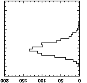
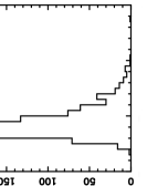
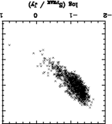
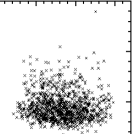
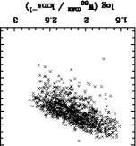
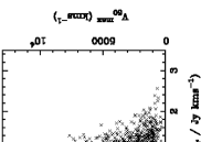
Figure 1: Log-log bivariate distributions of velocity width ($W_{\rm{50}}^{\rm{max}}$), peak flux ($S_{\rm{p}}$) and integrated flux ($S_{\rm{int}}$). Plotted along the diagonal are single parameter histograms.

NHICAT was constructed by first running the TopHat galaxy finder on all cubes, excluding the region $-300<v_{\rm{hel}}<300$ km s^-1 to minimise confusion with Galactic emission. 14,879 galaxy candidates were found. Each candidate source was then checked manually by simultaneously displaying the source in four ways: a spectrum, an integrated intensity map, a declination-velocity projection and a Right Ascension-velocity projection. A candidate source was accepted if it had a spectral profile which was easily distinguishable from the noisy baseline and a position-velocity profile which was wider than 2 pixels across the position axes. On the other hand, a candidate source was rejected if either its spectral profile was not distinguishable from the noise or if its position-velocity projections showed a distinct signal which was exactly 2 pixels wide, as these sources are usually the result of interference in the data. All the accepted sources were then passed to a semi-interactive parameter finder. Sources were flagged during parameter finding as either 1, 2, 3, 4 or a high-velocity cloud (HVC) detection: Flag=1 represented a definite source detection, 2 represented source detection with less certainty, 3 represented a source detected on the edge of a cube and 4 represented a non-detection. The Flag=4 option is provided to the parameter finder in the case of misclassification of a source during the checking stage. It should be noted that a significant number of HVCs were detected in Northern HIPASS at RA $\sim$ 23 hours due to the Magellanic stream. The Magellanic Stream from the Northern HIPASS data has been presented by Putman et al. (2003). Source lists from all cubes were then merged and duplicates were removed. The process of merging matched every Flag=3 source with the detection of the same source in the neighbouring cube with the same overlap region. The procedures for the manual checking and parametrisation used are exactly the same as MZ04. More detailed descriptions of these procedures can be found in sections 3.2 and 3.3 of MZ04. Bivariate distributions of the basic properties (heliocentric velocity, velocity width, peak flux and integrated flux) of the sources detected in Northern HIPASS are shown in Figure 1. Single parameter histograms are shown on the diagonal of this Figure.

The cubes were then re-checked for missed sources using a semi-interactive process. Sources detected in each cube were marked with a cross on an integrated intensity map. These maps were then manually checked for unmarked sources. From these manual checks, 15 additional sources were detected. The galaxy finder missed sources which were close to several other sources.

Two sources may also have been identified as the same source. Such sources can be differentiated by inspecting the spectra and the spatial moment maps since separate sources will not overlap both spatially and spectrally. These particular sources were flagged as ‘confused’. There are two ‘confused’ sources in NHICAT.

Extended sources were identified and fitted in the same fashion as in MZ04 (see section 3.5 of MZ04 for more details). All sources greater than $7\arcmin$ in size were identified as potentially extended sources. The integrated flux limit corresponding to a fixed source size can be determined using the relationship between integrated flux $S_{\rm{int}}$, and source diameter,

$$S_{\rm{int}}=\int SdV\approx 1.2\theta^{2}_{\mbox{\sc H{i}}}$$ (1)

An explanation and derivation of Equation 1 can be found in MZ04. The $S_{\rm{int}}$ limit corresponding to a source size greater than $7\arcmin$ is 57 Jy km s^-1 . In total, 41 candidates were found to have a measured flux greater than this limit. The moment maps of each of these sources were then examined and two sources were found to be extended.

All the cube velocities are heliocentric and use the optical definition where velocity,$v=c(f_{o}/f)/f$ where $c$, $f_{o}$ and $f$ represent the speed of light, rest and observed frequency respectively. The sources were then assigned names according to the convention of HICAT (Meyer et al., 2004).

The final stage of the processing involved checking the 19 sources located at $\delta<+2^{\circ}$. Of these, 18 sources have already been catalogued in HICAT showing that the datasets and analysis techniques are consistent between the two surveys at the 95% level. The extra source is located only slightly south of $\delta=+2^{\circ}$ and has been retained in NHICAT so that the final combined NHICAT and HICAT catalogue will be a complete catalogue of the southern skies up to $\delta=+25^{\circ}30\arcmin$.

Northern HIPASS covers 7997 square degrees of sky and 1002 galaxies were found from their Hi content in this region. The parameters provided with the catalogue are the same as the parameters given in HICAT. Detailed descriptions of each parameter can be found in Table 4 of MZ04.

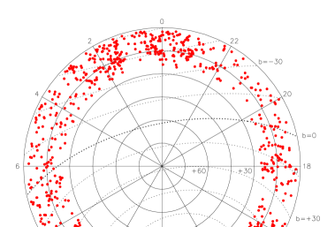
Figure 2: Skymap of detections found in Northern HIPASS. The lines mark increasing declinations inwards where the centre is the north pole. The radial divisions show increasing RA in an anti-clockwise direction starting with 0 hours at the top of the diagram. The dotted lines mark lines of Galactic latitude, $b$.

Figure 2 shows the spatial distribution of all the sources found in NHICAT. Note that the cluster of sources at RA, $\alpha\sim 12$ hours is the Virgo cluster. Galaxies are also found at low Galactic latitudes - a region often avoided by optical galaxy surveys. As mentioned in the introduction, NHIZOA (Donley et al. (2005)) covers a subset of the Northern HIPASS survey region. We re-identify 23 galaxies from the NHIZOA catalogue in the overlapping regions. The RMS of NHIZOA is 2.33 times less than that of the observations in Northern HIPASS. Assuming that the detected number of galaxies is based solely on the sensitivity of the observations, one would expect Northern HIPASS to find only 33 of the 77 NHIZOA sources. There are fewer matches between Northern HIPASS and NHIZOA because the source detection rate is not fully described by the sensitivity (as explained in the following section).

In accordance with HICAT conventions, NHICAT only included detections with $v_{\rm{hel}}>300$ km s^-1 . One galaxy, HIPASSJ1213+14a, was found to have a mean Hi $v_{\rm{hel}}$ of -222.7 km s^-1 , $S_{\rm{peak}}=0.181$ Jy and $S_{\rm{int}}=42.9$ Jy km s^-1Ṫhis galaxy was detected because its velocity width extended into the heliocentric velocity range where $v_{\rm{hel}}<-300$ km s^-1İn summary, no galaxies with $v_{\rm{hel}}<-300$ km s^-1 were found in NHICAT. The number density of the sources found in Northern HIPASS was approximately 0.13 sources per square degree of sky. In comparison, 0.20 sources per square degree of sky were found in Southern HIPASS. The cause of this difference will be discussed later in this paper.

Table 2: Comparison of source number density in NHICAT and HICAT. Note that 1 source in NHICAT was detected below $2^{\circ}$ in declination.

Catalogue	Declination range	Area of sky (sq degs)	No. of sources	Number density (per sq degs)
HICAT	$-90^{\circ}<\delta<+2^{\circ}$	21,346	4,315	0.20
NHICAT	$+2^{\circ}\leq\delta<+10^{\circ}$	2,862	413	0.14
	$+10^{\circ}\leq\delta<+18^{\circ}$	2,792	364	0.13
	$+18^{\circ}\leq\delta<+25^{\circ}$	2,343	224	0.10

2.2 Noise characteristics

Fewer sources were detected in NHICAT at higher declinations than in HICAT, as can be seen in Table 2 (which shows the number density in NHICAT and HICAT). Although some deviation is expected due to cosmic variance, the most likely cause of this density difference is the higher level of noise in Northern HIPASS. The variation in gain and system temperature ($T_{\rm{sys}}$) of the telescope with respect to elevation are insufficient to account for the higher noise observed in the northern survey. The level of noise in Northern HIPASS is greater than in Southern HIPASS because the Parkes radio telescope observes northern sources at lower sky elevations. This results in the telescope gathering a greater amount of interference from ground reflections and the Sun. As the most northerly areas of the survey were only observable during a short LST window, sidelobe solar interference was often unavoidable.

Figure 3: Peak-normalised distributions of pixel flux of entire cubes in HIPASS. The distribution of the pixel flux from a typical northern cube (cube number 538) is represented by crosses and the distribution marked by asterisks represent the pixel flux from a typical southern cube (cube number 194). A parabola (solid line) is shown to compare these distributions with Gaussian noise statistics.

As shown in Table 1, the RMS of both Northern and Southern HIPASS are very similar. However, the Northern HIPASS cubes appeared much ‘noisier’ in the flux density maps than that of the cubes in Southern HIPASS. Hence, the RMS method is not an effective way of illustrating why Northern HIPASS appeared ‘noisier’.

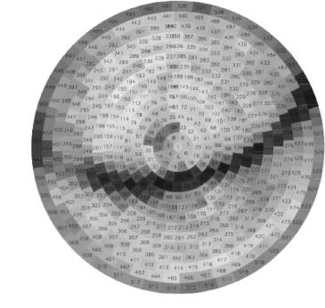
Figure 4: Skymap of the 1-percentile pixel flux map of both Northern and Southern HIPASS. The south pole ($\delta=-90^{\circ}$) is in the centre and RA increases in an anti-clockwise direction starting with 0 hour at the top of the diagram. Observations through the Galaxy (where $b=0^{\circ}$) correspond to the darker horizontal band of cubes. The southern cube identification numbers range from 1-388 and the northern cubes are 389-538.

Figure 5: Normalised histograms of ‘noise’ levels (1-percentile measures). The distribution of ‘noise’ levels in Southern HIPASS is represented by the solid line distribution. The dashed line distribution represents the ‘noise’ levels in the declination band between $+2^{\circ}<\delta<+10^{\circ}$ and the dotted line distribution represents the ‘noise’ levels in the declination bands between $+10^{\circ}<\delta<+26^{\circ}$.

The aim of this section is to characterise the distribution of noise observed in Northern HIPASS cubes. One method is to examine the distribution of all the pixel flux values in a given cube and measure the 99-percentile value of this distribution. This measure illustrates the noise characteristics in a given cube by measuring the extent of the outlying pixel flux values in the pixel distribution. Instead of characterising the noise in terms of the width of the flux distribution (as in the RMS method), we now examine the extent to which the outlier population is extended.

Figure 3 shows the peak-normalised pixel flux distributions of 2 average cubes, one from Northern HIPASS (cube number 538) and the other from Southern HIPASS (cube number 194). Since Hi detections comprise very few pixels compared with the entire cube, the Hi sources have not been removed from the plot. The excess of negative flux in Northern cubes (as seen in Figure 3) is due to the bandpass removal and calibration method. Negative bandpass sidelobes occur at declinations either side of bright sources (Barnes et al., 2001). This means that bright interference is surrounded by negative artifacts, leading to an excess of both positive and negative pixels in the data with stronger interference. An ideal cube with only Gaussian noise would have a parabolic distribution (as shown by the solid line) since the natural log of a Gaussian distribution, exp($-x^{2}$), is $-x^{2}$. As can be seen in Figure 3, the offset from the parabola is greater in the Northern cube than in the Southern cube, suggesting broader distributions of pixel noise values in the North.

Thus the ‘noise’ level can now be characterised by measuring the extent of outliers using the 99-percentile rank of the pixel flux distribution. In actuality, the $1$-percentile rank has been used to avoid bias caused by actual Hi sources in this measure. Figure 4 shows the skymap of the $1$-percentile measures for both Northern HIPASS and Southern HIPASS. It should be noted that the 3 outer bands of declinations (cube numbers 389 - 538) form the regions observed in Northern HIPASS, and the inner declination bands (cube numbers 1 - 388) represent the observed regions in Southern HIPASS.

It is qualitatively obvious from Figure 4 that observations through the Galaxy appear much ‘noisier’ than observations away from the Galaxy. It can also be seen that the northernmost declination band in Northern HIPASS is much noisier than the rest of the HIPASS observations.

Figure 6: Completeness of NHICAT as a function of $S_{\rm{p}}$, $W_{\rm{50}}$ and $S_{\rm{int}}$.

Table 3: Completeness of NHICAT.

Parameter	Completeness Fit	C=0.95
$S_{\rm{p}}$ (Jy)	erf$[18.5(S_{\rm{p}}-0.02)]$	0.095
$S_{\rm{int}}$ (Jy km s-1 )	erf$[0.1(S_{\rm{int}}-1.0)]$	15.0
$S_{\rm{p}}$(Jy), $S_{\rm{int}}$ (Jy km s-1 )	erf$[20.0(S_{\rm{p}}-0.005)]$erf$[0.14(S_{\rm{int}}-1.0)]$

A quantitative version of Figure 4 is as shown in Figure 5 with three normalised distributions of cube ‘noise’ levels (characterised by $1$-percentile rank). The cube ‘noise’ levels of Southern HIPASS are represented by the solid line distribution; the dashed and dotted line represent cube ‘noise’ level distributions of Northern HIPASS. The cube ‘noise’ level of the southernmost declination band in Northern HIPASS is shown by the dashed line distribution and the cube ‘noise’ level of the rest of Northern HIPASS is shown by the dotted line distribution. The median ‘noise’ level for the solid line and dashed line distributions are at 42 mJy and 43 mJy respectively and the median ‘noise’ level for the dotted line distribution (northernmost HIPASS) is 55 mJy. By this measure, the noise level has increased by $31\%$.

In conclusion, the ‘noisiness’ observed in the Northern HIPASS cube can be described quite accurately using the 1-percentile rank which measures the values of the pixel flux outliers in each cube. As mentioned before, the increase in the 1-percentile rank values for the northernmost declination band in Northern HIPASS is most likely a result of the increase in solar interference from increasingly lower elevation observations.

3 Completeness and reliability of NHICAT

The techniques used to calculate the completeness and reliability in NHICAT are the same as the methods used for HICAT. Detailed descriptions of the methods used to analyse the completeness and reliability of HICAT can be found in Zwaan et al. (2004).

3.1 Completeness of NHICAT

Synthetic sources were inserted into all the Northern HIPASS cubes before NHICAT was constructed in order to measure the completeness of the resulting catalogue. These synthetic sources were then extracted after the parameter finding process. In total, 774 non-extended synthetic sources were inserted into the Northern HIPASS cubes. These sources represent a random sample of sources ranging in $50\%$ velocity width ($W_{\rm{50}}$) from 20 to 650 km s^-1 , from 0.02 to 0.13 Jy in peak flux ($S_{\rm{p}}$) and from 300 to 10000 km s^-1 in heliocentric velocity ($v_{\rm{hel}}$).

The completeness of recovery can be easily estimated by measuring the fraction of fake sources (recovered in each parameter bin), $D$:

$$D(S_{\rm{p}},W)=N^{\rm{fake}}_{\rm{recovered}}(S_{\rm{p}},W)/N^{\rm{fake}}(S_{\rm{p}},W)$$ (2)

However, the completeness as a function of one parameter cannot be effectively measured solely using $D$. The completeness, $C$, of NHICAT can be measured via the ratio of the number of detected real sources, $N$, over the true number of sources in each bin. The true number of sources in each bin can be estimated by $N/D$. Since the number of sources in each bin differs and the parameter distribution of the fake sources may be different from the distribution of the real galaxies, this method cannot give a very good estimate of the completeness as a function of one parameter. A correction can be made by integrating over another parameter and applying a weighting to account for the different number of sources in each bin. As an example, $C(S_{\rm{p}})$ can be estimated by integrating over $W$ :

$$C(S_{\rm{p}})=\frac{\Sigma^{\infty}_{\rm{W=0}}N(S_{\rm{p}},W)}{\Sigma^{\infty}_{\rm{W=0}}N(S_{\rm{p}},W)/D(S_{\rm{p}},W)}$$ (3)

Likewise, $C(W)$ and $C(S_{\rm{int}})$ have been calculated by integrating over $S_{\rm{p}}$ . Figure 6 shows the completeness of NHICAT as functions of $S_{\rm{p}}$, $W$ and $S_{\rm{int}}$ respectively where the solid lines are error function fits to the datapoint. The error bars on the datapoints were determined using bootstrap re-sampling and show 68 percent confidence levels. The error function fits and the completeness limits at $95\%$ confidence levels are given in Table 3. Using the same method as Zwaan et al. (2004), different fitting functions were tested in order to fit the completeness as a function of two parameters. The completeness of NHICAT as a function of $S_{\rm{p}}$(Jy) and $S_{\rm{int}}$ (Jy km s^-1 ) is also shown in Table 3.

The completeness ($C(S_{\rm{p}})$) limits at $95\%$ confidence level is at 68 mJy for HICAT, while NHICAT’s completeness at the same confidence level is 91 mJy. It appears that to first order, the completeness of $S_{\rm{p}}$ scales with the noise level. However, it would be too simplistic to assume that the noise levels and source detection scale linearly . It should also be noted that cosmic variance has not been taken into account.

3.2 Reliability of NHICAT

The reliability of NHICAT was measured by re-observing a subsample of NHICAT sources in the narrowband mode at the Parkes Telescope. As with the reliability estimation of HICAT (Zwaan et al., 2004), a random sample representing the full range of NHICAT parameters was chosen, while giving preference to NHICAT detections with low $S_{\rm{int}}$ and $S_{\rm{p}}$ (generally with $S_{\rm{int}}<8$ Jy km s^-1 and $S_{\rm{p}}<0.07$ Jy).

3.2.1 Narrowband observations

In addition to calculating the reliability of NHICAT, the narrowband observations were also used to remove spurious detections from the catalogue. As such, the less certain source detections (Flag=2) were observed as higher priority. In addition, definite source detections (Flag=1) were chosen randomly by the observer for observation. These narrowband observations took place over 4 observing sessions from July 2003 to February 2005.

A spectral resolution of 1.65 km s^-1 at $z=0$ was used by observing with the narrow-band mode which consisted of 1024 channels over 8 MHz. Integration times were approximately 15 minutes for each source. The specific details of the observing mode used can be found in Zwaan et al. (2004). The narrowband observations were reduced using the AIPS++ packages livedata and gridzilla (Barnes et al., 2001) as with the narrowband observations of HICAT.

The percentage of rejected sources in the NHICAT narrowband observations was greater than for HICAT. A likely explanation is that the signal-to-noise level is less in the north and thus source detection algorithm is less effective than in the south.

A total of 857 sources were observed, of which 172 ($20\%$) were rejected, compared with the narrowband observations of HICAT where less than $10\%$ of the observed sources were rejected. Figure 7 shows the peak flux distributions of the follow-up observations in both Northern and Southern HIPASS. As can be seen from this figure, more sources were rejected at $S_{\rm{peak}}>0.05$ Jy in the Northern follow-up observations than in the Southern follow-up observations. Also, the percentage of sources with $S_{\rm{peak}}>0.05$ observed in the Southern follow-up observations are higher than in the Northern observations which may also explain the difference in the percentage rejected.

Figure 7: Peak flux, $S_{\rm{peak}}$ (Jy), distributions of the follow-up observations in Northern HIPASS (left) and in Southern HIPASS (right). The distributions marked with lines on a 45 degree angle represent the population of observed and confirmed detections, while, the distributions marked with horizontal lines represent the population of non-detected sources.

3.2.2 Reliability measure

As explained in Zwaan et al. (2004), the reliability will improve when more uncertain sources are removed after the narrowband follow-up observations. Therefore we start by examining the original catalogue before unconfirmed sources were removed. The ratio of the number of confirmed sources ($N^{\rm{rel}}_{\rm{conf}}$) to the number of observed sources ($N^{\rm{rel}}_{\rm{obs}}$) is defined to be :

$$T(S_{p},W)=N^{\rm{rel}}_{\rm{conf}}(S_{\rm{p}},W)/N^{\rm{rel}}_{\rm{obs}}(S_{\rm{p}},W)$$ (4)

The reliability $R$ as a function of a single parameter is the mean of $T$, weighted by the number of sources in each bin. For example the reliability as a function of peak flux ($S_{\rm{p}}$) is:

$$R(S_{\rm{p}})=\frac{\Sigma^{\infty}_{\rm{W=0}}N(S_{\rm{p}},W)\times T(S_{\rm{p}},W)}{\Sigma^{\infty}_{\rm{W=0}}N(S_{\rm{p}},W)}$$ (5)

Similarly, $R(W)$ and $R(S_{\rm{int}})$ can be measured by integrating over $S_{\rm{p}}$.

Figure 8: Reliability of NHICAT as a function of $S_{\rm{p}}$, $W_{\rm{50}}$ and $S_{\rm{int}}$. The histograms show the $S_{\rm{p}}$, $W_{\rm{50}}$ and $S_{\rm{int}}$ distributions of NHICAT sources.

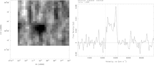
Figure 9: Example of 3 data products available online at $\langle$http://hipass.aus-vo.org$\rangle$ for source HIPASSJ0030+02. Clockwise from top left: Integrated intensity map, Hi spectra and a position-velocity projection intensity map.

Since $20\%$ of the observed sources in the initial NHICAT have been rejected and removed from the catalogue, the reliability of the catalogue has been improved by re-observing a subsample of the sources.

An estimate of the expected number of real sources has to be made in order to calculate the reliability of NHICAT after the removal of unconfirmed sources. The expected number of sources is given by:

$$N_{\rm{expectreal}}=N_{\rm{confirmed}}+(T\times N_{\rm{unobserved}})$$ (6)

where $N_{\rm{unobserved}}$ is the number of sources that have not been reobserved.

T can now be redefined as :

$$T(S_{\rm{p}},W)=\frac{N_{\rm{expectreal}}(S_{\rm{p}},W)}{N(S_{\rm{p}},W)}$$ (7)

where $N(S_{\rm{p}},W)$ is the total number of sources in NHICAT excluding the unconfirmed sources. Equation 5 can now be used to calculate the reliability of the final NHICAT.

Figure 4 shows the $S_{\rm{p}}$, $W$ and $S_{\rm{int}}$ distributions of NHICAT sources as well as the reliability of NHICAT as functions of $S_{\rm{p}}$, $W$ and $S_{\rm{int}}$ where the dashed lines are error function fits to the datapoint. It should be noted that 871 sources, 1002 sources and 764 sources are plotted in the $S_{\rm{p}}$, $W$ and $S_{\rm{int}}$ distributions, respectively. This is due to the fact that the rest of the sources have $S_{\rm{p}}$ and $S_{\rm{int}}$ greater than the parameter ranges given in Figure 4. The error bars on the datapoints were determined using bootstrap re-sampling and indicate 68 percent confidence levels. The error function fits and the completeness limits at $95\%$ confidence levels are given in Table 4.

Table 4: Reliability of NHICAT.

Parameter	Reliability Fit	C=0.95
$S_{\rm{p}}$ (Jy)	erf$[58(S_{\rm{p}}-0.012)]$	0.036

It is interesting though to note that the $95\%$ level of reliability in NHICAT is lower (in $S_{\rm{p}}$ and $S_{\rm{int}}$) than the $95\%$ level of reliability in HICAT. This result can be attributed to the fact that a larger proportion of the original NHICAT have been re-observed in the narrowband follow-up observations.

4 Summary

In the northern extension of HIPASS, which covers the region between declinations $+2^{\circ}<\delta<+25^{\circ}30\arcmin$, 1001 extragalactic sources were found and catalogued in NHICAT. In addition an extra source found with $\delta$ slightly less than $+2^{\circ}$ (which was not detected in HICAT) has also been included into NHICAT.

NHICAT has been found to be $95\%$ complete at peak flux 95 mJy and at an integrated flux 15 Jy km s^-1 . This catalogue is also reliable at a $95\%$ level at peak flux 36 mJy. The entire catalogue and source spectra will be made publicly-available online at $\langle$http://hipass.aus-vo.org$\rangle$. The catalogue parameters presented in the online archive are the same 33 parameters detailed in Table 4 of Meyer et al. (2004). An excerpt of the online catalogue is shown in Table 5. The online archive also contains the detection spectra and integrated intensity maps in various projections. Examples of these data products are shown in Figure 9. In addition to the Aus-VO archive, the catalogue and spectra will also be submitted to the NASA/IPAC Extragalactic Database (NED).

Chapter Acknowledgments.

The Multibeam system was funded by the Australia Telescope National Facility (ATNF) and an Australian Research Council LIEF grant. The HIPASS collaboration was partially supported by an ARC grant (DP0208618). The collaborating institutions are the Universities of Melbourne, Western Sydney, Sydney and Cardiff, Research School of Astronomy and Astrophysics at Australian National University, Jodrell Bank Observatory and the ATNF. The Multibeam receiver and correlator was designed and built by the ATNF with assistance from the Australian Commonwealth Scientific and Industrial Research Organisation Division of Telecommunications and Industrial Physics. The original low noise amplifiers were provided by Jodrell Bank Observatory through a grant from the UK Particle Physics and Astronomy Research Council.

We thank N. Bate, A. Karick, E. MacDonald, M. J. Pierce, R. M. Price, N. Rughoonauth, S. Singh, D. Weldrake and M. Wolleben for their help with the Parkes narrow-band follow-up observations. Finally, we would like to thank the staff at the Parkes Observatory for all their support.

Table 5: Excerpt from NHICAT. Note that all the velocities are $cz$ and heliocentric.

Name	RA	Dec	$v_{50}^{\rm{max}}$ (km s-1)	$v_{50}^{\rm{min}}$ (km s-1)	$v_{20}^{\rm{max}}$ (km s-1)	$v_{20}^{\rm{min}}$ (km s-1)	$v_{\rm{mom}}$ (km s-1)
	$v_{\rm{S_{p}}}$ (km s-1)	$v_{\rm{gsr}}$ (km s-1)	$v_{\rm{lg}}$ (km s-1)	$v_{\rm{cmb}}$ (km s-1)	$v_{\rm{lo}}$ (km s-1)	$v_{\rm{hi}}$ (km s-1)	$v_{\rm{speclo}}$ (km s-1)
	$v_{\rm{spechi}}$ (km s-1)	$v_{\rm{mask}}$ (km s-1)	$W_{50}^{\rm{max}}$ (km s-1)	$W_{50}^{\rm{min}}$ (km s-1)	$W_{20}^{\rm{max}}$ (km s-1)	$W_{20}^{\rm{min}}$ (km s-1)	$S_{\rm{p}}(Jy)$
	$S_{\rm{int}}(Jy\mbox{km s${}^{-1}$})$	RMS (Jy)	RMSClip (Jy)	RMSCube (Jy)	Cube	Sigma (km s-1)	Box size (′)
	Comment	Follow-up	Confused	Extended
HIPASSJ0030+02	00:30:00.6	02:05:46	762.0	5509.0	5347.5	765.3	5362.3
	5514.5	5370.3	5344.9	5336.2	5111.8	5590.2	4055.5
	6973.1	5112,5590	361.8	73.5	434.8	434.8	0.060
	13.5	0.0065	0.0049	0.01209	389	12	7
	1	1	0	0
HIPASSJ0033+02	00:33:44.3	02:40:37	4340.8	4454.8	4390.4	4336.6	4402.7
	4478.3	4411.8	4386.3	4377.6	4242.8	4542.0	2989.5
	5941.5	4243,4542	225.9	94.6	248.0	248.0	0.069
	9.5	0.0080	0.0073	0.01222	390	12	7
	1	1	0	0
HIPASSJ0142+02	01:42:28.4	02:56:20	2988.9	1763.9	1764.0	2989.1	1762.8
	1744.6	1772.0	1746.6	1737.9	1685.4	1843.3	321.3
	3221.2	1685,1843	80.6	80.6	109.9	109.9	0.112
	9.0	0.0070	0.0058	0.01362	392	12	7
	1	0	0	0
HIPASSJ0150+02	01:50:15.2	02:18:58	1503.8	1695.8	1696.6	1505.4	1696.0
	1677.9	1703.0	1677.6	1668.9	1618.9	1750.0	255.4
	3127.1	1619,1750	73.0	73.0	94.9	94.9	0.053
	3.5	0.0065	0.0060	0.01362	392	12	7
	1	1	0	0
HIPASSJ0249+02	02:49:06.4	02:08:27	1024.6	1104.7	1103.6	1023.3	1104.5
	1105.4	1113.8	1088.4	1079.7	1047.8	1167.3	-324.4
	2536.0	1048,1167	58.6	58.6	81.0	81.0	0.945
	55.6	0.2363	0.0543	0.01380	394	12	7
	1	0	0	0
HIPASSJ0253+02	02:53:48.6	02:20:42	3645.8	6787.8	-9999.0	3634.9	6730.6
	6833.6	6739.1	6713.7	6705.0	6532.9	6924.2	5129.9
	8319.0	6533,6924	349.4	235.8	0.000	0.000	0.037
	9.2	0.0072	0.0066	0.01440	395	12	7
	1	1	0	0
HIPASSJ0254+02	02:54:05.6	02:57:22	6731.0	2952.5	3039.7	-9999.0	3036.2
	2937.1	3043.9	3018.5	3009.8	2864.7	3212.5	1490.0
	4603.0	2865,3212	264.4	93.4	293.6	293.6	0.090
	17.1	0.0075	0.0063	0.01440	395	12	7
	1	0	0	0
HIPASSJ0259+02	02:59:48.2	02:45:38	376.0	2793.6	2848.4	-9999.0	2844.4
	2762.3	2850.4	2825.0	2816.4	2668.9	3025.0	1516.0
	4384.8	2669,3025	242.6	137.5	307.0	307.0	0.088
	16.9	0.0075	0.0069	0.01440	395	12	7
	1	0	0	0

References

- Barnes et al. (2001) Barnes D. G., Staveley-Smith L., de Blok W. J. G., Oosterloo T., Stewart I. M., Wright A. E., Banks G. D., Bhathal R., et al. 2001, MNRAS, 322, 486
- Donley et al. (2005) Donley J. L., Staveley-Smith L., Kraan-Korteweg R. C., Islas-Islas J. M., Schröder A., Henning P. A., Koribalski B., Mader S., et al. 2005, AJ, 129, 220
- Doyle et al. (2005) Doyle M. T., Drinkwater M. J., Rohde D. J., Pimbblet K. A., Read M., Meyer M. J., Zwaan M. A., Ryan-Weber E., et al. 2005, MNRAS, 361, 34
- Giovanelli et al. (2005) Giovanelli R., Haynes M. P., Kent B. R., Perillat P., Catinella B., Hoffman G. L., Momjian E., Rosenberg J. L., et al. 2005, AJ, 130, 2613
- Kenney et al. (2004) Kenney J. D. P., van Gorkom J. H., Vollmer B., 2004, AJ, 127, 3361
- Kilborn et al. (2002) Kilborn V. A., Webster R. L., Staveley-Smith L., Marquarding M., Banks G. D., Barnes D. G., Bhathal R., de Blok W. J. G., et al. 2002, AJ, 124, 690
- Koribalski et al. (2004) Koribalski B. S., Staveley-Smith L., Kilborn V. A., Ryder S. D., Kraan-Korteweg R. C., Ryan-Weber E. V., Ekers R. D., Jerjen H., et al. 2004, AJ, 128, 16
- Meyer et al. (2005) Meyer M. J., Zwaan M. A., Webster R. L., Brown M. J. I., Staveley-Smith L., 2005, in preparation
- Meyer et al. (2004) Meyer M. J., Zwaan M. A., Webster R. L., Staveley-Smith L., Ryan-Weber E., Drinkwater M. J., Barnes D. G., Howlett M., et al. 2004, MNRAS, 350, 1195(MZ04)
- Putman et al. (2003) Putman M. E., Staveley-Smith L., Freeman K. C., Gibson B. K., Barnes D. G., 2003, ApJ, 586, 170
- Rosenberg & Schneider (2002) Rosenberg J. L., Schneider S. E., 2002, ApJ, 567, 247
- Springob et al. (2005) Springob C. M., Haynes M. P., Giovanelli R., 2005, ApJ, 621, 215
- Staveley-Smith et al. (1996) Staveley-Smith L., Wilson W. E., Bird T. S., Disney M. J., Ekers R. D., Freeman K. C., Haynes R. F., Sinclair M. W., et al. 1996, Proc. Astron. Soc. Aust., 13, 243
- Vollmer et al. (2001) Vollmer B., Cayatte V., Balkowski C., Duschl W. J., 2001, ApJ, 561, 708
- Zwaan et al. (2005) Zwaan M. A., Meyer M. J., Staveley-Smith L., Webster R. L., 2005, accepted for publication in MNRAS
- Zwaan et al. (2004) Zwaan M. A., Meyer M. J., Webster R. L., Staveley-Smith L., Drinkwater M. J., Barnes D. G., Bhathal R., de Blok W. J. G., et al. 2004, MNRAS, 350, 1210
- Zwaan et al. (2003) Zwaan M. A., Staveley-Smith L., Koribalski B. S., Henning P. A., Kilborn V. A., Ryder S. D., Barnes D. G., Bhathal R., et al. 2003, AJ, 125, 2842