Old open clusters as key tracers of Galactic chemical evolution. I. Fe abundances in NGC 2660, NGC 3960, and Berkeley 32

Abstract

Aims. We obtained high-resolution UVES/FLAMES observations of a sample of nine old open clusters spanning a wide range of ages and Galactocentric radii. The goal of the project is to investigate the radial metallicity gradient in the disk, as well as the abundance of key elements ($\alpha$ and Fe-peak elements). In this paper we present the results for the metallicity of three clusters: NGC 2660 (age $\sim$ 1 Gyr, Galactocentric distance of 8.68 kpc), NGC 3960 ($\sim$1 Gyr, 7.80 kpc), and Be 32 ($\sim$6–7 Gyr, 11.30 kpc). For Be 32 and NGC 2660, our study provides the first metallicity determination based on high-resolution spectra.

Methods. We performed equivalent width analysis with the spectral code MOOG, which allows us to define a metallicity scale and build a homogeneous sample.

Results. We find that NGC 3960 and NGC 2660 have a metallicity that is very close to solar ([Fe/H]=+0.02 and +0.04, respectively), while the older Be 32 turns out to have [Fe/H]=$-$0.29.

1 Introduction

The investigation of chemical abundances in stars is fundamental for comprehending the Galaxy formation mechanisms and the subsequent evolution. In recent years, several observational and theoretical studies have been carried out, aimed at understanding various features, such as the star formation history in the disk and its Galactocentric distribution, the gas distribution and stellar density, the metallicity distribution ([Fe/H]) in the disk, as well as the abundances of other elements relative to Fe (e.g. Edvardsson et al. edvar (1993); Friel et al. friel03 (2003); Carretta et al. carretta04 (2004), carretta05 (2005); Yong, Carney, & de Almeida yong05 (2005)). Although many observational characteristics of the Milky Way are reproduced well by the appropriate theoretical models (Lacey & Fall lacey (1985); Tosi tosi88 (1988); Giovagnoli & Tosi giova (1995); Chiappini, Matteucci, & Gratton chiappini97 (1997); Boissier & Prantzos boissier (1999)), several problems persist.

One of these problems concerns the radial metallicity gradient in the disk, i.e. the distribution of chemical elements with Galactocentric distance ($R_{\rm{gc}}$) and its evolution with age. The radial metallicity gradient and its temporal evolution are among the most critical constraints on Galactic chemical evolution models, since predictions of its slope and slope variations with time depend mainly on the relative timescales of the gas consumption (i.e. star formation rate) and gas accretion (i.e. infall rate), that is with the disk formation scenario. At the same time, the abundances of $\alpha$ and Fe-peak elements and their ratios to Fe are crucial for getting insight into the role of stars with different masses and evolutionary lifetimes in the heavy element enrichment of the interstellar medium.

The distribution of heavy elements with Galactocentric distance is often investigated through observations of objects like H ii regions and B stars (e.g. Shaver et al. shaver (1983); Smartt & Rollerstone smartt (1997)), which are bright and measurable also in external galaxies. They show a negative gradient, but it is not clear if the slope changes with position in the disk and, given the young ages of all these objects, it is impossible to evaluate whether it varies with age. Good indicators are also planetary nebulæ (PNe); observations of type ii PNe (whose progenitors are $\sim$2–3 Gyr old) reveal the presence of a gradient similar to that traced by H ii regions, but its precise slope is still under debate (e.g. Pasquali & Perinotto perinotto (1993); Maciel, Costa, & Uchida maciel (2003)), since the investigation of PNe is affected by the uncertainty on their distances. In our opinion, one of the best tools for the investigation of radial abundance distributions is represented by open clusters, since they cover a wide range of ages, metallicities, and positions in the Galactic disk.

Various observational studies have already addressed the problem of the metallicity distribution through open cluster observations, but the general picture has not been delineated well yet, and discrepant results have been obtained by different authors. For example, Friel (friel95 (1995); friel_cast (2006)), Carraro, Ng, & Portinari (carraro98 (1998)) and Friel et al. (friel02 (2002)) suggest the presence of a negative [Fe/H] gradient, while Twarog, Ashman, & Anthony-Twarog (twarog (1997)) and Corder & Twarog (corder (2001)) favor a step-like distribution of the Fe content with Galactocentric distance. Furthermore, recent results (e.g., Yong et al. yong05 (2005)) suggest that a single slope is not a good fit to the data when clusters farther than about 14 kpc from the center are included. Even when restricted to metallicities derived by spectroscopic data, large differences appear to be present among different analyses.

The discrepancies among the various literature results can be ascribed to several concurring factors: the number of stars employed (statistics), the quality of the spectra (signal-to-noise – $S/N$ – and spectral resolution) and, above all, the method of analysis, including continuum tracing, atomic parameters, equivalent width ($EW$) measurement, model atmospheres, spectral code, and atmospheric parameters. Diverse methods of analysis and physical assumptions are adopted by different authors, so that the resulting chemical abundances have been often referred to discrepant scales of temperature and metallicity. An investigation of this kind instead needs to rely on a large sample of open clusters for which element abundances (but also distances and ages) are derived with the same method in order to avoid spurious results due to an inhomogeneous analysis.

Although the number of open clusters studied with high-resolution spectroscopy is steadily increasing, we still lack a suitable sample for deriving truly reliable constraints on the gradient and its evolution with time. To this aim and in the context of a VLT/FLAMES program on Galactic open clusters (Randich et al. messenger (2005)), we collected UVES spectra of evolved stars in a variety of old open clusters. Our sample includes To~2 ($\sim$2–3 Gyr), NGC~6253 ($\sim$3 Gyr), Be~29 ($\sim$4 Gyr), Be~20 ($\sim$5 Gyr), Be~32 ($\sim$6–7 Gyr) and NGC~2324, NGC~2477, NGC~2660, NGC~3960 (ages $\lesssim$ 1 Gyr). Likewise $R_{\rm{gc}}$ varies between $\sim$7 and 21 kpc (Be 29 being the most distant cluster found so far). The primary goal of the UVES observations is to determinate the metallicity of the sample clusters using a homogeneous method of analysis: in this way, we will have a new rather large sample with all the clusters on the same abundance scale. At the same time we derive – in most cases for the first time – abundances of other key elements, as CNO, $\alpha$, and Fe-peak elements, as well as s- and r-process elements, which are fundamental for understanding Galactic formation and evolution.

The emphasis of this paper is on presenting the method of analysis for [Fe/H] and on determining the metallicity of three of the open clusters included in the project (NGC 3960, NGC 2660, Be 32). The analysis of $\alpha$ elements and Fe-peak elements in the same clusters and in NGC 2477, NGC 2324 is deferred to a forthcoming paper (Bragaglia et al. 2006b, in preparation). NGC 3960 was recently investigated through high-resolution spectroscopy by Bragaglia et al. (2006a – hereafter B06a), therefore it is well-suited to directly comparing it with another spectroscopic analysis and to estimating possible sources of discrepancies between different studies at high resolution. As far as the other clusters are concerned, neither NGC 2660 nor Be 32 have ever been studied using high-resolution spectroscopy.

The paper is organized as follows: in Sect. 2 we present the properties of the target clusters and in Sect. 3 we describe observations and data reduction. In Sect. 4 we give a detailed description of the method of analysis and inputs adopted (e.g., line lists and atomic parameters). The results for Fe abundances in the three open clusters are reported in Sect. 5 and discussed in Sect. 6. A summary closes this paper (Sect. 7).

2 Target clusters

Table 1: Target clusters and their properties. Literature sources are reported in the text.

Cluster	Age	[Fe/H]	$R_{\rm{gc}}$	$(m-M)_{0}$	$E(B-V)$
	(Gyr)		(kpc)	(mag)	(mag)
NGC 3960	0.9$\rightarrow$1.4	$-$0.68$\rightarrow$$-$0.06	7.80	11.60	0.29 (differential)
NGC 2660	$\sim$1	solar/sub-solar	8.68	12.20	0.40
Be 32	$\sim$6$\rightarrow$7	$-$0.50$\rightarrow$$-$0.37	11.30	12.48	0.10

The main properties of the three open clusters investigated in this paper are reported in Table 1.

NGC 3960 is located at a Galactocentric distance $R_{\rm{gc}}=7.8$ kpc. The first CMD for the cluster was published by Janes (janes81 (1981)), based on $BV$ photographic data. More recently, Prisinzano et al. (prisinzano (2004)) investigated this cluster by collecting data in the $BVI$ bands with the Wide Field Imager at the ESO-Max Planck 2.2m telescope. These authors found strong indications of differential reddening in the direction of the cluster, with $E(B-V)$ varying from 0.16 to 0.62 over their $\approx$ 30 $\times$ 30 arcmin² field of view. They found $E(B-V)=0.29$ towards the cluster center (in agreement with Janes janes81 (1981)), $(m-M)_{0}=11.35$, and age ranging from 0.9 to 1.4 Gyr. The most recent work on NGC 3960 is the photometric and spectroscopic study by B06a, who find $(m-M)_{0}=11.60$ and an average $E(B-V)=0.29\pm 0.02$ (over a field of view of 13.3 $\times$ 13.3 arcmin²), with differential reddening of $\pm$0.05 mag (in agreement with the values inferred by Prisinzano et al. in their central region, corresponding to B06a field of view) and a slightly sub-solar metallicity, [Fe/H]=$-$0.12. This is the only metallicity estimate based on high-resolution spectroscopy. Previous reports suggested a lower Fe content: for example, Friel & Janes (fj93 (1993)) quoted [Fe/H]=$-$0.34 from low-resolution spectroscopy. Other estimates range from [Fe/H]=$-$0.68 (Geisler, Clarià, & Minniti geisler (1992); from Washington photometry) to $-$0.06 (Piatti, Clarià, & Abbadi piatti (1995), using a DDO abundance calibration). NGC 3960 has been included in several other studies; for example, by Twarog et al. (twarog (1997)), who determined a metallicity of $-$0.17, based on a homogenization of DDO photometry and low-resolution spectroscopy, and by Mermilliod et al. (mermi01 (2001)), who determined precise radial velocities for a number of red giants.

NGC 2660 was first investigated by Hartwick & Hesser (hh73 (1973); photographic and photoelectric study), and a more recent analysis was performed by Sandrelli et al. (sandrelli (1999)), who presented CCD $UBVI$ photometry and estimated an age of $\sim$ 1 Gyr or slightly less, a distance modulus $(m-M)_{0}=12.20$, and reddening $E(B-V)\sim 0.40$, implying a Galactocentric distance of 8.68 kpc (Bragaglia & Tosi bt06 (2006)). The cluster metallicity has been investigated by various authors but only on the basis of photometry, and with inconsistent results: Sandrelli et al. (sandrelli (1999)) quoted a nearly solar Fe content (from stellar evolutionary tracks), while previous works reported a sub-solar [Fe/H] (e.g., Hesser & Smith hs87 (1987); Piatti et al  piatti (1995), both from DDO photometry).

As pointed out in Sect. 1, the main goal of this project is to investigate the radial metallicity gradient in the disk and its temporal evolution. Be 32 is $\sim$6–7 Gyr old, which is relevant for the evolution of the gradient with age. Although the most distant cluster in our sample is Be 29 ($R_{\rm{gc}}\sim 21$ kpc), Be 32 is the most distant among the three clusters analyzed in this paper and, with a Galactocentric radius $>$ 10 kpc, it is located beyond the [Fe/H] vs. $R_{\rm{gc}}$ discontinuity found by Twarog et al. (twarog (1997)). Therefore, Be 32 is the most interesting of the three clusters. Photometric studies of the cluster were carried out by Kaluzny & Mazur (kal (1991)), Richtler & Sagar (rich (2001)), Hasegawa et al. (hasegawa (2004)) and D’Orazi et al. (dorazi (2006)). The last study finds reddening and distance modulus $E(B-V)=0.10$ and $(m-M)_{0}=12.48$. As for the metal content, a sub-solar Fe has been suggested for the cluster, e.g., by Noriega-Mendoza & Ruelas-Mayorga (noriega (1997)), who found [Fe/H]=$-$0.37 based on the CMD, by Friel et al. (friel02 (2002)) based on low-resolution spectroscopy ([Fe/H]=$-$0.50), and by D’Orazi et al. (dorazi (2006)) based on evolutionary tracks ($Z$=0.008).

3 Observations and data reduction

The open clusters included in the program were all observed with the multi-object instrument FLAMES on VLT/UT2 (ESO, Chile; Pasquini et al. P00 (2000)). The fiber link to UVES was used to obtain high-resolution spectra ($R=40,000$) for red giant branch (RGB) and clump objects.

NGC 3960 was observed in Service mode in 2004; two FLAMES configurations were used, and UVES observations were performed for both configurations with two different gratings (CD3 and CD4, covering the wavelength ranges $\sim$4750–6800 Å and 6600–10600 Å, respectively). A log of observations (date, UT, exposure time, grating, configuration, number of stars) is given in Table 2. The spectra were reduced by ESO personnel using the dedicated pipeline, and we analyzed the 1-d, wavelength-calibrated spectra using standard IRAF packages.

Table 3 provides information on the target stars. We observed 7 red clump and 3 main sequence (MS) stars, but we only present here the results for the giants. We adopt hereafter the provisional identification number used for FLAMES pointing (Col. 1); however, since $BVI$ photometry was taken from Prisinzano et al. (prisinzano (2004)), we also show in Col. 2 the ID from their catalogue. $J$ and $K$ magnitudes come from the Two Micron All Sky Survey (2MASS; Cutri et al. cutri (2003)). The MS stars were eventually discarded since they are rather faint, too warm (late A or early F spectral type), and rotate too rapidly. They are also not suitable for a detailed chemical abundance analysis, since the $S/N$ is too low and their lines are broad and shallow.

Radial velocities were measured using RVIDLINES on several tens of metallic lines on the individual spectra, then multiple spectra were combined. One fiber for configuration was used to register the sky value, but the correction was negligible. We corrected the spectra for the contamination by atmospheric telluric lines using TELLURIC in IRAF and an early-type star observed with UVES for another program. The $RV$s for each star (shown in Table 3) have an attached uncertainty of less than about 0.5 km s^-1, as deduced from the rms when averaging values obtained from different exposures; this error is also valid for the two other clusters. We derived an average heliocentric $RV$ of $-22.6\pm 0.9$ (statistical error) km s^-1 for NGC 3960. Star c1 turned out to be a non-member on the basis of the radial velocity and spectral characteristics and is disregarded from now on (see also Mermilliod et al. mermi01 (2001)). Star c8 is a long-period spectroscopic binary (star 50 in Mermilliod et al. mermi01 (2001)), so its radial velocity appears slightly discrepant with respect to the cluster average; nevertheless it is compatible with it, once the amplitude of the $RV$ curve is considered. The spectral features and average metallicity (see Sect. 5) clearly indicate that c8 is a cluster member.

Table 2: Observation log of NGC 3960. One star is common to configurations A and B; we consider only clump objects here (7 stars in total). The remaining fibers were assigned to sky and to MS stars.

Date	UTbeginning	Exposure time	Configuration	Grating	no. of stars
		(s)			(clump)
2004-04-03	02 57 39.980	2595	A	CD4	4
2004-04-03	03 52 16.186	2595	A	CD4	4
2004-04-03	04 47 31.818	2595	A	CD3	4
2004-04-20	03 37 39.635	2595	B	CD3	4
2004-05-02	00 12 31.740	2595	B	CD4	4
2004-05-02	00 57 37.007	2595	B	CD4	4
2004-05-02	01 43 13.805	2595	B	CD3	4
2004-05-02	02 39 18.200	2595	A	CD3	4

Table 3: Data for NGC 3960. ID_phot and $BVI$ photometry (non corrected for differential reddening) are from Prisinzano et al. (prisinzano (2004)).The number of exposures for each star is intended as the number of pointings with the same cross-disperser.

Star	Star	RA	DEC	$B$	$V$	$I$	$J_{\rm{2MASS}}$	$K_{\rm{2MASS}}$	no. exp.	$RV$	$S/N$	Notes
IDfla	IDphot									(km s-1)
c1	310753	11 50 06.330	$-$55 44 13.00	15.866	14.262	12.496	11.213	10.238	2	+1.83	60–80	NM
c3	310755	11 50 33.149	$-$55 42 36.13	14.799	13.514	12.088	11.079	10.357	2	$-$24.16	120–130	M
c4	310756	11 50 28.184	$-$55 41 36.66	14.366	13.194	11.907	10.989	10.304	2	$-$22.39	95–115	M
c5	310757	11 50 36.050	$-$55 42 05.40	14.323	13.062	11.679	10.671	9.959	2	$-$21.94	110–130	M
c6	310758	11 50 26.750	$-$55 40 28.20	14.084	12.945	11.697	10.815	10.133	4	$-$21.86	115–160	M
c8	310760	11 50 37.621	$-$55 40 15.19	14.224	13.060	11.758	10.820	10.162	2	$-$32.87	120–190	bin, M
c9	310761	11 50 38.100	$-$55 39 44.50	14.309	13.100	11.787	10.839	10.151	2	$-$22.58	100–110	M

Be 32 and NGC 2660 were observed in Visitor mode in 2005 January 19–22, and a log of the observations is given in Table 4. Be 32 was targeted using two FLAMES configurations, For configuration A, the observations were carried out with both CD3 and CD4 gratings, while only CD3 was employed for configuration B For NGC 2660, we got only one exposure with the CD3 grating. The spectra were reduced by us, using the dedicated UVES pipeline (Mulas et al. uves_pipeline (2002)). Since observations were performed at full Moon and in the presence of cirrus, the background signal is high; nevertheless, we were able to carry out a good background subtraction using, as is customary, the fibers dedicated to the sky. Information on radial velocities and photometry are recorded in Tables 5 and 6 for Be 32 (10 stars) and NGC 2660 (5 stars), respectively.

In Table 5 we report the provisional ID for the stars used for the FLAMES pointing (adopted in the following) and those from the photometry by D’Orazi et al. (dorazi (2006)). Note that for star 938 the photometry was retrieved from Kaluzny & Mazur (kal (1991)) and that star 932 turned out to be a non-member, because of both its $RV$ and its spectral features; therefore it has been dropped from the analysis. Identification numbers and $BVI$ magnitudes for NGC 2660 (listed in Table 6) were taken from Sandrelli et al. (sandrelli (1999)).

The average heliocentric $RV$s for Be 32 and NGC 2660 are $<RV>=+106.0\pm 1.4$ km s^-1 and $<RV>=+21.2\pm 0.6$ km s^-1, respectively. The $S/N$ given in Tables 3, 5, 6 refers to the spectra centered at 5800 Å, on which our analysis rests, measured using the task SPLOT within IRAF. Considering the wavelength regions around $\sim$5600 and 6300 Å, the final combined spectra of NGC 3960 have typical $S/N\sim$100–160; lower values result for Be 32, which has $S/N\sim$50–100. Finally, spectra of NGC 2660, for which only one exposure for each star was available, have typical $S/N$ of $\sim$45–70.

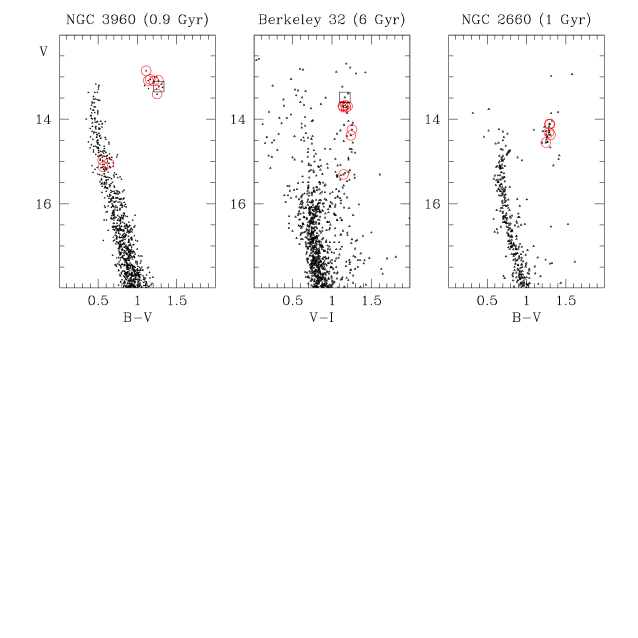
Figure 1: Color-magnitude diagrams for the three clusters. From left to right: NGC 3960, Be 32, and NGC 2660. Note that the first and the last clusters are reported in the ($B-V$, $V$) plane, while Be 32 is in the ($V-I$, $V$) one. The observed stars are shown by circles (members) and squares (non-members).

Figure 1 shows the CMDs for the three open clusters in the ($B-V$, $V$) plane for NGC 3960 and NGC 2660, while for Be 32 we considered the ($V-I$) colors because the $B$ magnitude of star 938 is not available. Circles (members) and squares (non-members) mark the stars observed with UVES.

We show the spectra of all the clump stars in the sample (cluster members) in Figs. 2, 3, and 4. For clarity we restricted the plot to a region of $\sim$100 Å at 6500–6600 Å.

Table 4: Observation log of Be 32 and NGC 2660. One star is common to configurations A and B in Be 32 (10 stars in total). The remaining fibers were assigned to the sky.

Cluster	Date	UTbeginning	Exp.time	Config.	Grating	no. of stars
			(s)
Be 32	2005-01-20	00 47 00	3600	A	CD3	7
Be 32	2005-01-20	02 01 53	3600	A	CD4	7
Be 32	2005-01-20	03 11 03	3600	A	CD4	7
Be 32	2005-01-20	04 23 41	3600	A	CD3	7
Be 32	2005-01-21	00 45 26	3600	B	CD3	4
NGC 2660	2005-01-23	08 02 02	3600	–	CD3	5

Table 5: Data for Be 32. ID_phot, and $BVI$ are from D’Orazi et al. (dorazi (2006)), while ID_fla is the identification number used for FLAMES observations.

Star	Star	RA	DEC	$B$	$V$	$I$	$J_{\rm{2MASS}}$	$K_{\rm{2MASS}}$	no. exp.	$RV$	$S/N$	Notes
IDfla	IDphot									(km s-1)
17	533	6 58 8.242	6 24 19.48	14.754	13.667	12.540	11.683	11.028	2	105.3	80–100	M
18	997	6 58 13.762	6 27 54.89	14.730	13.661	12.534	11.709	11.069	2	105.5	80–100	M
19	787	6 58 3.089	6 26 16.08	14.800	13.709	12.564	11.722	11.024	2	101.4	70–90	M
25	121	6 57 59.819	6 26 59.93	15.387	14.242	13.028	12.153	11.450	1	105.5	45–60	M
27	605	6 58 2.262	6 24 56.71	15.511	14.372	13.177	12.282	11.607	2	105.6	60–70	M
45	1139	6 58 7.473	6 29 32.67	16.299	15.278	14.153	13.341	12.707	3	105.3	45–50	M
932	1183	6 58 1.771	6 29 55.32	14.450	13.425	12.282	11.474	10.843	2	30.8	90–100	NM
938	-	6 58 11.488	6 21 16.25	-	13.672*	12.501*	11.686	11.027	1	106.1	50–60	M
940	104	6 58 22.909	6 26 25.26	14.793	13.691	12.535	11.691	11.023	1	105.0	70–75	M
941	99	6 57 50.572	6 26 11.92	14.769	13.663	12.477	11.643	10.973	2	105.5	85–95	M

*$V$ and $I$ from Kaluzny & Mazur (kal (1991)).

Table 6: Data for NGC 2660. ID and $BVI$ photometry are from Sandrelli et al. (sandrelli (1999)).

. Star RA DEC $B$ $V$ $I$ $J_{\rm{2MASS}}$ $K_{\rm{2MASS}}$ $RV$ $S/N$ Notes (km s^-1) 296 8 42 36.411 $-$47 12 07.26 15.798 14.552 13.174 11.680 10.636 21.73 45–65 M 318 8 42 36.693 $-$47 10 37.06 15.401 14.110 12.713 11.586 10.828 20.66 50–65 M 542 8 42 41.704 $-$47 11 25.22 15.420 14.120 12.704 11.603 10.837 20.47 45–90 M 694 8 42 45.418 $-$47 11 18.71 15.674 14.368 12.938 11.791 11.049 21.47 45–55 M 862 8 42 50.651 $-$47 13 03.61 15.602 14.315 12.909 11.770 11.046 21.47 50–70 M

4 Abundance analysis

The analysis of chemical abundances was carried out with the last version (2005) of the spectral program MOOG (Sneden sneden (1973)) and using model atmospheres by Kurucz (kuru (1993)). Like all the commonly used spectral analysis codes, MOOG performs a local thermodynamic equilibrium (LTE) analysis.

4.1 Solar analysis

The first step is the determination of the solar Fe abundance, which allows us to fix a zero-point for the metallicity scale. This differential analysis minimizes errors in the results, especially for stars with nearly solar metallicity.

The line list adopted for the Sun is the one used by Gratton et al. (G03 (2003) – hereafter G03), which includes 180 and 40 features for Fe i and Fe ii, respectively, in the wavelength range $\sim$4100–6800 Å. Either theoretical or laboratory oscillator strengths ($\log gf$) were considered, retrieved from the works by the Oxford group (e.g. Blackwell et al. oxford (1986)), and from Bard, Kock, & Kock (bard91 (1991)), O’Brian et al. (obrian91 (1991)), and Bard & Kock (bard94 (1994)). Most of the equivalent widths adopted for the Sun are from Rutten & Van der Zalm (rutten (1984)), who performed measurements on the Sacramento Peak Irradiance Atlas (Beckers, Bridges, & Gilliam sacramento (1976)); this set was integrated with measurements performed by G03 on the solar spectrum atlases by Delbouille, Roland, & Neven (atlas_del (1973)) and by Kurucz (atlas_kuru (1984)). Note that the solar spectra employed have much higher resolution than our UVES spectra.

When available, we adopted collisional damping coefficients from Barklem, Piskunov, & O’Mara (barklem (2000)), who provide the best theoretical models for most transitions. When the coefficients by Barklem et al. were not available we considered classical damping constants ($C_{6}$) computed with the approximation of Unsöld (unsold (1955)) and multiplied by an enhancement factor E, given by: $\log E=(0.381\pm 0.017)EP-(0.88\pm 0.33)$. This expression was obtained by G03 from several hundred Fe i features with available accurate collisional damping parameters and for $T_{\rm eff}$=5000 K, typical of giant stars.

The line list for the Sun is available in electronic form; the table includes wavelengths, name of the element (Fe i or Fe ii), $EP$, $\log gf$, $EW$, and references for the damping coefficients. We computed the Fe content ($\log n(\rm{Fe})$) for the Sun by adopting the following effective temperature, surface gravity, and microturbulence velocity: $T_{\rm eff}$=5779 K, $\log g$=4.44, and $\xi$=0.8 km s^-1. The values of the solar microturbulence reported in the literature range from 0.8 to 1.1 km s^-1 (e.g. Randich et al. R06M67 (2006)). We chose 0.8 km s^-1, which is the best fit value reported by Grevesse & Sauval (GS99 (1999)); as well known, an increase in $\xi$ would result into a decrease of the solar $\log n(\rm{Fe})$. We derived $\log n(\rm{Fe}$ i)=7.49$\pm$0.04 (standard deviation, or rms) and $\log n(\rm{Fe}$ ii)=7.54$\pm$0.03, in good agreement with the estimates available in the literature (e.g., Grevesse & Sauval GS99 (1999); Asplund, Grevesse, & Sauval AS05 (2005)). Usual checks for the suitability of the adopted parameters are the excitation equilibrium and the plot of Fe abundance vs. $EW$s (see Sect 4.4). We find a negligible trend of the Fe i abundance with the excitation potential ($EP$) – hence the excitation equilibrium is satisfied (see Sect. 4.4) – while a slightly stronger trend is present considering $\log n(\rm{Fe}$ i) vs. the measured $EW$s (a positive slope of $\sim$0.06 in the plot of abundance vs. $\log(EW/{\lambda})$). In order to put the value of this slope to $\sim$0, we should have slightly enhanced the microturbulence (up to 0.95 km s^-1) and, as a consequence, the $T_{\rm eff}$ (up to 5800 K); in this case, the Fe abundance would have been 7.48. However, we decided to retain the initial parameters for the Sun as the right ones and therefore did not put the slopes of $\log n(\rm{Fe}$ i) vs. measured $EW$s and vs. $EP$ to zero. We warn the reader that this choice can lead to a systematic shift in the metallicity scale; had we assumed a lower $\log n(\rm{Fe}$ i), we would have found slightly higher metallicities for the open cluster stars.

Finally, we note that using the previous version (2002) of MOOG, where it is not possible to treat collisional damping with the Barklem coefficients, we would have obtained $\log n(\rm{Fe}$ i)=7.51$\pm$0.04 and $\log n(\rm{Fe}$ ii)=7.55$\pm$0.04 (considering classical damping constants from the Unsöld formula, in most cases multiplied by the enhancement factor $E$).

4.2 Line list for giant stars

The line list adopted for giant stars in open clusters (retrieved from G03) covers the wavelength range 5500–6800 Å for Fe i (157 lines) and 5500–6500 Å for Fe ii (15 lines). The Fe features included were first carefully selected by G03 in order to exclude the presence of severe blending. Moreover, very strong lines ($EW\mathrel{\hbox{\hbox to0.0pt{\hbox{\lower 4.0pt\hbox{$\sim$}}\hss}\hbox{$>$}}}150$ mÅ, see Sect. 4.3) have also been discarded, since they are critically sensitive to the microturbulence value; and further, a more detailed treatment of damping would be needed to fit the line wings. Note that, although the investigation by G03 concerned metal-poor halo stars, the line list adopted here was accurately tested and employed for solar metallicity open clusters (Carretta et al. carretta04 (2004), carretta05 (2005); B06a). Fe features at wavelengths bluer than $\sim$5500 Å were excluded to avoid complications by crowding and continuum tracing: therefore, $\sim$60 Fe i and $\sim$25 Fe ii lines used for the solar analysis are not included in the giant list. On the other hand, there are additional useful Fe i features with respect to the solar line list, in the list used for giants (since they are visible only in cool stars). Based on these facts, the analysis is not formally “differential” with respect to the Sun; however, as a test we measured the solar abundance using the lines shared by the two lists and found the same $\log n(\rm{Fe})$ values, reinforcing our method. More in detail, the fraction of Fe i features not included in the solar line list are about 25 % of the lines used for giants. This, in principle, might represent a systematic bias, since the excitation equilibrium of Fe i lines (and therefore the $T_{\rm eff}$) is strongly driven by the lowest and highest excitation lines. However, the majority of the features not shared by the Sun and giants have $EP$ in the range 3–5 eV, similar to those of the other lines present in the total lists (see also below). Only two lines in this subsample have very low $EP$ ($<2$ eV); therefore, the use of two different subsets of lines for the Sun and the giants does not represent a source of error.

Wavelengths, $EP$, and $\log gf$ for the lines used are reported in Table 7. A wide range in $EP$ and $\log gf$ (i.e., corresponding to a wide range of line strengths) is spanned at all wavelengths by Fe i features, with more than 70 % of the lines having $EP\geq 3$ eV and ${\log gf\geq-3}$; only 10 features have $EP$ lower than 2 eV and $\log gf$ lower than $-$4.

The sources for the treatment of damping are also reported: G03 (see Sect. 4.1), Barklem et al. (barklem (2000)), Unsöld (unsold (1955)) . Note that only in two cases (where the Barklem and G03 values were not available) was the classical Unsöld approximation used.

Table 7: Set of Fe lines adopted for the analysis.

Wavelength	$EP$	$\log gf$	Damping	Wavelength	$EP$	$\log gf$	Damping
(Å)	(eV)		source	(Å)	(eV)		source
Fe I				5806.732	4.610	-0.930	2
5494.474	4.070	-1.960	1	5811.912	4.140	-2.360	1
5521.281	4.430	-2.510	1	5814.815	4.280	-1.810	2
5522.454	4.210	-1.470	2	5835.109	4.260	-2.180	2
5524.244	4.150	-2.840	2	5837.702	4.290	-2.300	2
5539.291	3.640	-2.590	2	5849.687	3.690	-2.950	2
5547.000	4.220	-1.850	2	5852.228	4.550	-1.360	2
5552.687	4.950	-1.780	2	5853.150	1.480	-5.090	1
5560.220	4.430	-1.100	2	5855.086	4.610	-1.560	2
5568.862	3.630	-2.910	2	5856.096	4.290	-1.570	2
5577.028	5.030	-1.490	1	5858.785	4.220	-2.190	2
5586.771	3.370	-0.100	2	5859.596	4.550	-0.630	1
5587.581	4.140	-1.700	1	5861.110	4.280	-2.350	2
5595.051	5.060	-1.780	1	5862.368	4.550	-0.420	1
5608.976	4.210	-2.310	2	5879.490	4.610	-1.990	2
5609.965	3.640	-3.180	2	5880.025	4.560	-1.940	2
5611.357	3.630	-2.930	2	5881.279	4.610	-1.760	2
5618.642	4.210	-1.340	2	5902.476	4.590	-1.860	2
5619.609	4.390	-1.490	2	5905.680	4.650	-0.780	2
5635.831	4.260	-1.590	2	5927.797	4.650	-1.070	2
5636.705	3.640	-2.530	2	5929.682	4.550	-1.160	2
5649.996	5.100	-0.800	2	5930.191	4.650	-0.340	2
5651.477	4.470	-1.790	2	5933.805	4.640	-2.140	2
5652.327	4.260	-1.770	2	5934.665	3.930	-1.080	2
5661.017	4.580	-2.420	2	5947.531	4.610	-2.040	1
5661.354	4.280	-1.830	2	5956.706	0.860	-4.560	2
5677.689	4.100	-2.640	2	5976.787	3.940	-1.300	1
5678.388	3.880	-2.970	1	5984.826	4.730	-0.290	1
5680.244	4.190	-2.290	1	6003.022	3.880	-1.020	2
5701.557	2.560	-2.160	2	6007.968	4.650	-0.760	1
5717.841	4.280	-0.980	2	6008.566	3.880	-0.920	1
5731.772	4.260	-1.100	2	6015.242	2.220	-4.660	2
5738.240	4.220	-2.240	2	6019.369	3.570	-3.230	2
5741.856	4.260	-1.690	2	6027.059	4.070	-1.200	1
5742.963	4.180	-2.350	2	6056.013	4.730	-0.460	2
5752.042	4.550	-0.920	1	6065.494	2.610	-1.490	2
5754.406	3.640	-2.850	2	6078.499	4.790	-0.380	1
5759.259	4.650	-2.070	2	6079.016	4.650	-0.970	2
5760.359	3.640	-2.460	2	6082.718	2.220	-3.530	2
5775.088	4.220	-1.110	1	6089.574	5.020	-0.870	1
5778.463	2.590	-3.440	2	6093.649	4.610	-1.320	2
5784.666	3.400	-2.530	2	6094.377	4.650	-1.560	2
5793.922	4.220	-1.620	2	6096.671	3.980	-1.760	2

References: (1) Gratton et al. (G03 (2003); G03); (2) Barklem et al. (barklem (2000)); (3) Unsöld (unsold (1955)).

Table 7: (continued).

Wavelength	$EP$	$\log gf$	Damping	Wavelength	$EP$	$\log gf$	Damping
(Å)	(eV)		source	(Å)	(eV)		source
6098.250	4.560	-1.810	2	6581.218	1.480	-4.680	2
6120.258	0.910	-5.860	1	6591.314	4.590	-2.040	2
6137.002	2.200	-2.910	2	6593.884	2.430	-2.300	2
6151.623	2.180	-3.260	2	6608.044	2.280	-3.960	2
6157.733	4.070	-1.260	1	6609.118	2.560	-2.650	2
6165.363	4.140	-1.480	1	6625.039	1.010	-5.320	1
6173.341	2.220	-2.840	2	6627.560	4.550	-1.500	2
6187.402	2.830	-4.130	1	6633.758	4.560	-0.810	2
6187.995	3.940	-1.600	2	6667.426	2.450	-4.370	2
6199.509	2.560	-4.350	2	6667.723	4.580	-2.100	2
6200.321	2.610	-2.390	2	6699.142	4.590	-2.110	2
6213.437	2.220	-2.540	2	6703.576	2.760	-3.000	2
6219.287	2.200	-2.390	2	6704.485	4.220	-2.640	1
6220.791	3.880	-2.360	2	6713.745	4.790	-1.410	2
6226.740	3.880	-2.080	2	6725.364	4.100	-2.210	2
6232.648	3.650	-1.210	3	6726.673	4.610	-1.050	1
6240.653	2.220	-3.230	2	6733.153	4.640	-1.440	2
6246.327	3.600	-0.730	2	6739.524	1.560	-4.850	2
6252.565	2.400	-1.640	2	6745.965	4.070	-2.710	1
6265.141	2.180	-2.510	2	6750.164	2.420	-2.580	2
6270.231	2.860	-2.550	2	6753.465	4.560	-2.350	2
6280.622	0.860	-4.340	2	6756.547	4.290	-2.780	1
6290.548	2.590	-4.360	2	6786.860	4.190	-1.900	2
6297.799	2.220	-2.700	2	6793.260	4.070	-2.430	1
6301.508	3.650	-0.720	3	6796.120	4.140	-2.400	1
6303.466	4.320	-2.620	2	6804.297	4.580	-1.850	2
6311.504	2.830	-3.160	2	6806.856	2.730	-3.140	2
6315.814	4.070	-1.670	1	6810.267	4.610	-1.000	2
6322.694	2.590	-2.380	2	Fe ii
6330.852	4.730	-1.220	2	5525.135	3.270	-4.040	2
6335.337	2.200	-2.280	2	5534.848	3.240	-2.750	2
6380.750	4.190	-1.340	1	5627.502	3.390	-4.140	2
6392.538	2.280	-3.970	2	5991.378	3.150	-3.550	2
6393.612	2.430	-1.430	2	6084.105	3.200	-3.800	2
6400.323	3.600	-0.230	1	6113.329	3.210	-4.120	2
6411.108	4.730	-2.330	1	6149.249	3.890	-2.720	2
6411.658	3.650	-0.600	2	6239.948	3.890	-3.440	2
6421.360	2.280	-1.980	2	6247.562	3.870	-2.320	2
6436.411	4.190	-2.400	1	6369.463	2.890	-4.210	2
6481.878	2.280	-2.940	2	6383.715	5.550	-2.090	2
6498.945	0.960	-4.660	2	6416.928	3.890	-2.700	2
6518.373	2.830	-2.560	2	6432.683	2.890	-3.580	2
6533.940	4.560	-1.280	2	6456.391	3.900	-2.100	2
6574.254	0.990	-4.960	1	6516.083	2.890	-3.380	2

4.3 Equivalent widths

The continuum tracing and normalization of the spectra were carried out using the task CONTINUUM within IRAF, dividing the spectra in small regions (50 Å) and visually checking the output. The $EW$ measurements were carried out with the program SPECTRE, developed by Chris Sneden (see Fitzpatrick & Sneden spectre (1987)), which performs a Gaussian fitting of the line profiles. The values are available in electronic tables, where the first two columns list the wavelengths and element – Fe i or Fe ii – and the others show the corresponding $EW$ for each star.

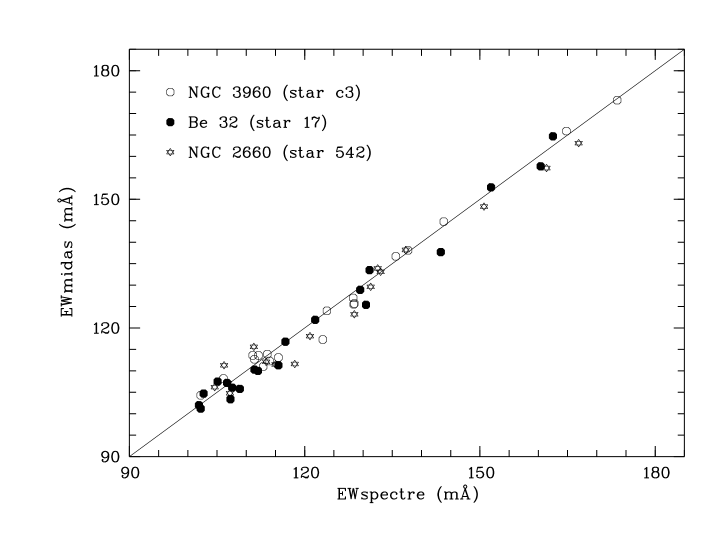
Figure 5: Comparison between $EW$ measured with SPECTRE and with MIDAS for strong Fe i lines in sample stars of the three clusters.

Continuum tracing and $EW$ determination are among the most critical steps in chemical abundance analysis, and they can represent the main reason for discrepancies between the results obtained by different authors (see Sect. 5). In particular, these steps are very problematic for metal-rich giant stars, which suffer from heavy line blending. We also mention that Gaussian fitting of the line profile is not always appropriate for strong lines; in those cases other fitting techniques, such as the use of a Voigt profile or a direct integration, would ensure that the contribution of damping wings is included in the measurement. Since the program SPECTRE does not allow performance of a fit different from Gaussian, we discarded lines with $EW$s larger than $\sim$ 150 mÅ (with the exception of a couple of cases, see Fig. 5). On the other hand, the Gaussian function produces a good fit of the lines with $EW$ in the range 100–150 mÅ. This has been proved by measuring the lines with strength in this interval also with the task INTEGRATE/LINE within the program MIDAS, which performs a direct integration of the spectral features. We report in Fig. 5 a comparison between the $EW$s measured with SPECTRE and MIDAS for three representative stars in the clusters. Note the very good agreement between the two sets of measurements for each star, indicating that the Gaussian fitting is appropriate for features not stronger than $\sim$150 mÅ.

4.4 Stellar parameters

Initial effective temperatures were derived from $B$, $V$, and $K$ photometry, applying the calibration by Alonso, Arribas, & Martinez-Roger (alonso (1999)), based on a large sample of field and open-cluster giant stars. The initial surface gravity was computed as $\log g=\log(M/M_{\odot})+0.4(M_{bol}-M_{bol{\odot}})+4{\cdot}\log(T_{\rm{eff}}/T_{\rm{eff}\odot})+\log g_{\odot}$, where $M$ is the mass and $M_{bol}$ the bolometric magnitude (with the symbol $\odot$ referring to the Sun and $M_{bol{\odot}}$=4.72). The clump masses were retrieved from the isochrones computed by the Padova group (Bertelli et al. padova (1994)): 1 $M_{\odot}$ for Be 32 (age $\sim$ 6 Gyr), and 2 $M_{\odot}$ for NGC 3960 and NGC 2660 (age $\sim$ 1 Gyr). We adopted indicative ages, but the surface gravity is only slightly affected by the choice of clump mass: for example, assuming 1.1 $M_{\odot}$ instead of 1.0 $M_{\odot}$ would imply a change of $\sim$0.04 dex in $\log g$.

In addition, the photometric $T_{\rm eff}$ and $\log g$ only represent starting values, whereas the two parameters were optimized during the spectral analysis. More specifically, we employed the driver ABFIND in MOOG to compute Fe abundances for the stars: the final effective temperature was chosen in order to eliminate possible trends in $\log n(\rm{Fe}$ i) vs. $EP$ (excitation equilibrium). As is well known, this method relies on the circumstance that, when the $T_{\rm eff}$ is over-estimated, the observed $EW$s of the lines with higher $EP$ are matched by a lower abundance, and vice versa.

The surface gravity was optimized by assuming the ionization equilibrium condition, i.e. $\log n(\rm{Fe}$ ii)$-$$\log n(\rm{Fe}$ i)=0.05 (as found for the Sun). Then, if necessary the $T_{\rm eff}$ was re-adjusted in order to satisfy both the ionization and excitation equilibria.

The choice of the microturbulence velocity deserves a more detailed description. In most of the chemical analysis present in the literature $\xi$ is optimized by minimizing the slope of the relationship between $\log n(\rm{Fe}$ i) and the observed $EW$s. This technique is based on the fact that strong lines are very sensitive to microturbulence: therefore, too high a $\xi$ would yield too low an abundance for strong lines. On the other hand, Magain (magain (1984)) showed that random errors in $EW$s lead to systematic over-estimation of the microturbulence. A possible method of obtaining an unbiased determination of $\xi$ is to optimize it by instead using the expected $EW$s, which are free from random errors. The theoretical $EW$s can be computed as $\log EW_{exp}=\log gf-EP\cdot(5040/(0.86\cdot{T_{\rm{eff}}}))$ mÅ, which is an approximation of a classical expression (Gray gray (1976)).

For simplicity and for self-consistency, we adopted a relation derived using the following procedure by Carretta et al. (carretta04 (2004)), who analyzed a sample of stars in three open clusters with nearly solar metallicity and derived a relationship between the final microturbulence velocities (optimized using the method suggested by Magain magain (1984)) and $\log g$. The resulting expression is $\xi=[1.5-0.13\times{\log g}]$ km s^-1. We tested this relationship for our sample of stars: namely, we constructed plots of $\log n(\rm{Fe}$ i) vs. expected $EW$s and found that the microturbulence obtained by zeroing the slope of this relationship is very similar to that which is computed following the prescriptions by Carretta et al. In fact, considering the whole sample of stars in the three clusters, we obtained a relationship between $\xi$ and $\log g$ that is almost identical to the expression reported above.

We also performed a comparison with a more commonly used analysis by optimizing the microturbulences using the $\log n(\rm{Fe}$ i) vs. observed $EW$s. We find reasonable differences between the final atmospheric parameters derived with the two techniques: in the worst cases we have $\Delta{\xi}\sim$0.15 km s^-1, $\Delta{T_{\rm{eff}}}\sim$80 K, $\Delta{\log g}\sim$0.3 dex, but generally average differences in $T_{\rm eff}$, microturbulence, and gravity do not exceed 50 K, 0.1 km s^-1, and 0.2 dex, respectively. Variations in the atmospheric parameters concur in different ways to changes in abundances, and the differences in the final Fe content are within $\pm$0.02 dex. Furthermore, we notice that in some cases the relationship $\log n(\rm{Fe}$ i) vs. observed $EW$ has a negligible slope, even if the microturbulence has been optimized in function of the expected $EW$s.

4.5 Errors

Our abundance scale is directly referred to the solar $\log n(\rm{Fe})$ and the majority of the spectral lines used for giants stars are in common with those included in the solar line list. In this way, internal errors due to uncertainties in the oscillator strengths should be minimized.

Random internal errors in $EW$s can be estimated by comparing the $EW$s of two stars with similar parameters. Considering the common lines between the two stars and rejecting significant outliers, we found the following average differences: $<\Delta{EW}>\pm{\delta}=-0.95\pm 2.54$ mÅ (where $\delta$ indicates the rms) for NGC 3960 (c3$-$c6; 112 lines), $-1.02\pm 3.75$ mÅ for Be 32 (17$-$794; 90 lines), and $-1.49\pm 4.48$ mÅ for NGC 2660 (318$-$862; 76 lines). The random errors in $EW$ are represented by ${\delta}/{\sqrt{2}}$ (assuming that they can be equally attributed to both stars in the pair under consideration), therefore we find that their values are $\sim$1.8, $\sim$2.7, and $\sim$3.2 mÅ for NGC 3960, Be 32 and NGC 2660, respectively.

The effect of random errors in $EW$s and of errors in the atomic parameters on the derived abundance for a single star is well-represented by $\sigma_{1}$, the standard deviation from the mean abundance based on the whole set of lines (see Table 8). However, Fe abundances are also affected by uncertainties on the adopted stellar parameters: the total error in [Fe/H] for each star, $\sigma_{\rm{tot}}$, can be computed by quadratically adding $\sigma_{1}$ to the error deriving from random uncertainties in $T_{\rm eff}$, $\log g$ and $\xi$, which we will call $\sigma_{2}$. Typical $\sigma_{2}$ values for each cluster can be estimated by varying one parameter at a time (holding the others fixed) and then by quadratically adding the three related errors, $\sigma_{T\rm{eff-rd}}$, $\sigma_{\log g-\rm{rd}}$, and $\sigma_{\xi-\rm{rd}}$ (see below).

Errors in $T_{\rm eff}$, $\log g$, and $\xi$ have been evaluated in the same fashion as in Carretta et al. (carretta04 (2004)). A detailed description of the method can be found in the quoted reference, but we mention here that we find standard total internal errors of $\sim$35 K in temperature for individual stars in the three clusters. The corresponding uncertainty in abundance ($\sigma_{T\rm{eff-TOT}}$) is the quadratic sum of the internal random term ($\sigma_{T\rm{eff-rd}}$, related to the $EW$ measurement) and the internal systematic term ($\sigma_{T\rm{eff-sys}}$). Using the formulas of Carretta et al., we estimated $\sigma_{T\rm{eff-rd}}$ to be 0.033, 0.055, and 0.066 dex for NGC 3960, NGC 2660, and Be 32, respectively, i.e. about 47 %, 69 % ,and 78 % of the total uncertainty. Therefore, the internal random errors in the temperatures are $\sim$15–25 K for individual stars in these clusters. Systematic scale errors are always difficult to estimate, and a more detailed discussion must be deferred to the completion of the analysis for our whole sample of clusters. At present, the good agreement between results from different approaches (photometric and spectroscopic) allows us to estimate that scale errors are likely to be confined typically within 100–150 K.

Errors in surface gravities are due to two contributions, one from spectroscopic effective temperatures, and the other from errors in the measurement of individual lines (see Carretta et al. carretta04 (2004)). The total (random + systematic) error $\Delta{\log g}$ results in 0.15–0.25 dex. Taking only the random part (i.e. 47, 69, and 78 % for NGC 3960, NGC 2660, and Be 32, respectively) of this error into account, we find that the total random uncertainty $\Delta{\log g}_{\rm{rd}}$ is 0.13 dex for NGC 3960, 0.10 dex for NGC 2660 and 0.12 dex for Be 32.

Errors in the microturbulence velocity are computed for a typical star in each cluster and depend on the variation in the slope of the adopted abundance vs. expected $EW$ relation and on the relationship between $\xi$ and $\log g$ (see Carretta et al. carretta04 (2004)). The random internal errors $\Delta{\xi}_{\rm{rd}}$ are $\sim$0.10 km s^-1 for NGC 3960, $\sim$0.17 km s^-1 for NGC 2660 and $\sim$0.20 km s^-1 for Be 32.

As already mentioned, $\sigma_{2}$ is the error in abundance related to random internal uncertainties in the stellar parameters, and it is due to three terms: $\sigma_{T\rm{eff-rd}}$, $\sigma_{\log g-{\rm rd}}$, and $\sigma_{\xi-{\rm rd}}$. The first term is reported above, while the two last are calculated by estimating the sensitivity of $\log n(\rm{Fe}$ i) to the following changes: $\Delta{\log g}_{\rm{rd}}$=0.10–0.13 dex and $\Delta{\xi}_{\rm{rd}}$=0.10–0.20 km s^-1. The sensitivity of [Fe/H] to errors in the stellar parameters is exemplified in Table 9: for each cluster we chose the star with Fe abundance and $T_{\rm eff}$ most similar to the average values. Note that we adopted sample parameter variations of $\pm$100 K in $T_{\rm eff}$, $\pm$0.2 dex in $\log g$ and $\pm$0.15 km s^-1 in $\xi$, even if different from the random errors in the stellar parameters estimated to compute $\sigma_{2}$ in our clusters.

The presence of systematic errors due to the method of analysis can be checked by analyzing stars with well-known metallicity, as for example the Hyades, and possibly observed with the same instrument. Unfortunately, we observed two Hyades stars (the clump objects $\gamma$ Tau and $\delta$ Tau) only with SARG at the TNG at lower resolution ($R\sim 29,000$). The same method described above was employed to carry out the analysis. We found similar abundances and parameters for the two stars, with $T_{\rm eff}$=4860 K, $\xi$=1.40 km s^-1, $\log g$=2.50, and [Fe/H]=+0.17$\pm$0.08 for $\gamma$ Tau, and $T_{\rm eff}$=4905 K, $\xi$=1.41 km s^-1, $\log g$=2.60, and [Fe/H]=+0.19$\pm$0.08 for $\delta$ Tau. Then $\xi$ was optimized using both the observed and expected $EW$. We note that using the parameters reported above we were indeed able to optimize the Fe abundance vs. $EW$s distribution for either expected and observed $EW$s.

Our value for the metallicity of the Hyades appears somewhat higher than most of the estimates present in the literature based on dwarfs: for example Boesgaard & Friel (bf90 (1990)) quoted [Fe/H]=+0.13 for MS stars, which is the most commonly accepted value. However, considering that they assume $\log n(\rm{Fe})_{\odot}$=7.56, higher by 0.07 than our value, our metallicity is perfectly consistent with theirs. In more recent analysis Boesgaard, Beard, & King (bbk (2002)) quote [Fe/H]=+0.16, while Paulson, Sneden, & Cochran (paulson (2003)) find [Fe/H]=+0.13. Recent investigations of giant stars are those by Smith (smith (1999): [Fe/H]=+0.15), by Wylie, Cottrell, & Taute (wylie (2004): [Fe/H]=+0.19), and by Schuler et al. (schuler (2006): [Fe/H]=+0.16), in agreement with our result.

5 Results

Our results for the Fe abundances are reported in Table 8. Columns 2 and 3 list the photometric $T_{\rm eff}$ derived from $(B-V)$ and $(V-K)$ colors, and the average of these two values was assumed as initial $T_{\rm eff}$ for the analysis for each star. In Col. 4 we report the photometric $\log g$ (mean value of gravities from $B-V$ and $V-K$ colors). For star 938 in Be 32 $BV$ photometry by D’Orazi et al. (dorazi (2006)) was not available; therefore, we adopted the $V$ magnitude by Kaluzny & Mazur (kal (1991)) and listed only $T_{\rm eff}$$(V-K)$. For star 296 in NGC 2660, the $K$ value is clearly wrong, leading to a $T_{\rm eff}$($V-K$) of 4300 K, very different from the $T_{\rm eff}$($B-V$) and from the temperatures of the other clump stars. For the whole sample, effective temperatures derived from ($B-V$) and ($V-K$) colors are in generally good agreement (i.e. within the errors), differing by 0–70 K in NGC 3960, by 20–150 K in Be 32, and by $\sim$100 K in NGC 2660.

The final stellar parameters determined via the spectroscopic analysis described in Sect. 4.4 are shown in Cols 5–7 ($T_{\rm eff}$, $\log g$ and $\xi$). In most cases, we found reasonable agreement between the photometric and spectroscopic parameters. The spectroscopic and (average) photometric temperatures usually coincide within $\sim$100 K.

As far as surface gravities are concerned, we note that to satisfy the ionization equilibrium, we had to consider a $\log g$ usually lower than the photometric ones. The differences have average values of $\Delta({\log g}_{\rm{phot}}-{\log g}_{\rm{spec}})$=0.30$\pm$0.12 (statistical error) for NGC 3960, 0.20$\pm$0.10 for Be 32, and 0.15$\pm$0.12 for NGC 2660. These differences are slightly larger than the errors in $\log g$ (see Sect. 4.5) and could be attributed to several random factors, such as internal errors, errors in distance moduli (0.2 mag translates into 0.08 dex in gravity), errors in reddenings (important especially for NGC 3960 where a differential reddening was noted by Prisinzano et al. 2004 and confirmed for the inner region by B06a at the level of $\pm$0.05 mag, corresponding to $\Delta{\log g}\sim 0.07$ dex), errors in ages (i.e., in masses, although the contribution is rather small), non homogeneity of the data sources, etc. Another possible explanation for the difference between spectroscopic and photometric gravities might be represented by non-LTE effects and/or inadequacies in classical (1-d) model atmospheres where important features such as spots, granulation, activity, etc. are neglected. Such a discrepancy has also been encountered by other authors (Feltzing & Gustafsson feltzing (1998); Schuler et al. schuler03 (2003); Allende Prieto et al. allende04 (2004)) in studies of cool metal-rich stars. Nevertheless, random uncertainties might not be the only reason for the discrepancies between photometric and spectroscopic gravities, as also a systematic error due to the method of analysis could probably be present. The microturbulence values, derived as described in Sect. 4.4, cover a rather narrow range in each cluster, as expected from the fact that clump stars are in the same evolutionary status.

In the last three columns of Table 8, we report the Fe abundance with respect to the Sun ([Fe/H]), and their errors: $\sigma_{1}$ and $\sigma_{\rm{tot}}$. $\sigma_{\rm{tot}}$ are computed by quadratically adding $\sigma_{1}$ and $\sigma_{2}$ as discussed in Sect. 4.5. We estimated typical $\sigma_{2}$ values in the three clusters of $\sim$0.05 dex for NGC 3960, and 0.08–0.09 dex for the other two clusters. When determining Fe abundances of the stars, 1$\sigma$-clipping was performed as the first step, that is, before the optimization of the stellar parameters.

The average (weighted mean) values for the clusters are also given, with the standard deviation from the mean (considering the total uncertainty $\sigma_{\rm{tot}}$). NGC 3960 turns out to have a solar metallicity, $<$[Fe/H]$>$=$+0.02\pm 0.04$ dex, at variance with some previous reports of sub-solar Fe content (see the discussion in Sect. 6.1). NGC 2660 also has a solar Fe content: $<$[Fe/H]$>$=$+0.04\pm 0.04$, while for Be 32 we derive a mean value $<$[Fe/H]$>$=$-0.29\pm 0.04$ in fair agreement with previous estimates of sub-solar metallicity.

Plots of the Fe abundance as a function of $T_{\rm eff}$ are shown in Fig. 6 for each cluster. Error bars ($\sigma_{\rm{tot}}$) are also reported. The resulting abundances are characterized by a small dispersion. This is only in part due to the 1-$\sigma$ clipping performed during the first iteration of the analysis; indeed, most of the lines discarded during that step were common to the various stars. Typical $\sigma_{1}$ values before the clipping were about 0.15 dex (i.e. twice the final $\sigma_{1}$).

Table 8: Stellar parameters (photometric and spectroscopic) and Fe abundances for the sample stars in the three clusters.

Star	$T_{\rm eff}$(B-V)	$T_{\rm eff}$(V-K)	$\log g_{\rm{phot}}$*	$T_{\rm eff}$spec	$\log g_{\rm{spec}}$	$\xi$	[Fe/H]	$\sigma_{1}$	$\sigma_{\rm{tot}}$
	(K)	(K)		(K)		km s-1
NGC 3960
c3	4814	4743	2.78	4950	2.35	1.19	+0.00	0.08	0.09
c4	5047	5027	2.78	5050	2.54	1.17	+0.07	0.07	0.09
c5	4862	4769	2.62	4870	2.16	1.22	+0.00	0.07	0.09
c6	5120	5121	2.72	4950	2.4	1.19	+0.02	0.08	0.09
c8	5064	5017	2.73	5040	2.57	1.18	+0.00	0.07	0.09
c9	4968	4959	2.71	5000	2.45	1.18	+0.02	0.08	0.09
Average Fe							+0.02		0.04 (rms)
Be 32
17	4830	4738	2.45	4830	2.22	1.21	$-$0.31	0.07	0.11
18	4866	4784	2.47	4850	2.27	1.21	$-$0.27	0.08	0.12
19	4822	4694	2.45	4760	2.26	1.21	$-$0.35	0.08	0.12
25	4718	4598	2.61	4760	2.40	1.19	$-$0.20	0.10	0.13
27	4729	4622	2.67	4780	2.35	1.19	$-$0.24	0.08	0.12
45	4964	4905	3.15	4920	3.00	1.11	$-$0.35	0.10	0.13
938	–	4732	2.45	4870	2.33	1.19	$-$0.30	0.09	0.13
940	4800	4710	2.45	4800	2.10	1.23	$-$0.33	0.09	0.13
941	4793	4690	2.43	4760	2.40	1.19	$-$0.29	0.08	0.13
Average Fe							$-$0.29		0.04 (rms)
NGC 2660
296	5126	–	3.01	5200	3.01	1.11	+0.08	0.09	0.12
318	5028	4926	2.75	5030	2.59	1.16	0.00	0.07	0.11
542	5008	4925	2.76	5060	2.48	1.17	+0.03	0.07	0.11
694	4996	4886	2.85	5100	2.77	1.14	+0.05	0.08	0.11
862	5036	4940	2.85	5100	2.60	1.16	+0.02	0.09	0.12
Average Fe							+0.04		0.04 (rms)

*Photometric gravities are the average between $\log g$ from $(B-V)$ and $(V-K)$.

Table 9: Sensitivities of Fe abundances to variations in the atmospheric parameters for typical stars in the three clusters.

Star	$\sigma_{T\rm{eff}}$	$\sigma_{\log g}$	$\sigma_{\xi}$
	$\Delta$$T_{\rm eff}$=$\pm$100 K	$\Delta{\log g}$=$\pm$0.2 dex	$\Delta{\xi}$=$\pm$0.15 km s-1
c9 (NGC 3960)	+0.09/$-$0.06	+0.01/0.00	$-$0.05/+0.06
17 (Be 32)	+0.09/$-$0.07	+0.01/0.00	$-$0.05/+0.06
542 (NGC 2660)	+0.09/$-$0.07	+0.01/0.00	$-$0.05/+0.06

6 Discussion

6.1 Comparison with previous studies

Using the synthetic CMD technique, Sandrelli et al. (sandrelli (1999)) found for NGC 2660 that all the best-fit models for the three adopted sets of stellar evolutionary tracks were obtained for solar metallicity. For Be 32, Friel et al. (friel02 (2002)) derived [Fe/H]=$-$0.50 from low-resolution spectra. Sub-solar metallicity has also been found by Kaluzny & Mazur (kal (1991)) on the basis of photometry ([Fe/H]=$-$0.37$\pm$0.05) and by D’Orazi et al. (dorazi (2006)) who derived a best-fit metallicity $Z=0.008$ ([Fe/H]$\sim-$0.40). While our results are reasonably consistent with the previous ones, it is important to emphasize that we provide the first metallicity reports for these two open clusters based on high-resolution spectroscopic data.

As far as NGC 3960 is concerned, literature reports based on photometry or low resolution spectroscopy quoted a clearly sub-solar Fe content (Friel & Janes fj93 (1993); Geisler, Clarià, & Minniti geisler (1992); Piatti, Clarià, & Abbadi piatti (1995)). The discrepancy with these results is probably due to the difference in the reliability of the method of analysis and quality of the data, so we think it is not worth undertaking a detailed comparison. On the other hand, we can perform a direct comparison with the very recent study by B06a, who carried out a spectroscopic analysis (Fe and other elements) for three stars in the cluster, observed with the FEROS spectrograph at the 1.5m ESO telescope in La Silla (Chile). The three objects in common with our sample are c5, c6 and c8. While the $S/N$ ratio of their spectra is lower than ours, the spectral resolving power of the two instruments is comparable.

The same line list (with the same $\log gf$ and damping parameters) was used to determine the Fe abundances; furthermore, the same concepts for optimizing the stellar parameters were adopted. Nevertheless, the two methods of analysis differ in other important steps: the determination of the continuum and $EW$ measurement and the adopted spectral code (the package ROSA, developed by Gratton ROSA (1988) has been used by B06a). Detailed descriptions of the method of analysis adopted by B06a can be found in Bragaglia et al. (bragaglia01 (2001)), G03, and Carretta et al. (carretta04 (2004)).

The comparison between our results and those by B06a is presented in Table 10, where a very good agreement between the spectroscopic parameters derived by the two methods is evident. In the last column we list the difference among the net $\log n(\rm{Fe})$ values from the two studies. Note that B06a have $\log n(\rm{Fe}$ i)_⊙=7.54 and $\log n(\rm{Fe}$ ii)_⊙=7.49 for the Sun (while we find Fe ii to be higher than Fe i, see Sect. 4.1). We carefully checked the reasons for this difference between the solar Fe content derived with MOOG and ROSA: in the case of neutral Fe, the abundance obtained with ROSA for the Sun is systematically higher, for both strong and weak lines. Had we found higher differences in the case of strong lines, this could have been related to a faulty treatment of damping. The difference between the abundances of ionized Fe goes instead in the opposite direction with respect to Fe i. We therefore tentatively conclude that the discrepancy of $\pm$0.05 dex among the two solar analyses could be due to a systematic difference between the two combinations of spectroscopic code and model atmospheres. Considering this, the average difference between the metallicity obtained by us and by B06a for the three stars in common is 0.07 dex (our estimate minus the B06a one).

By comparing the $EW$ sets for each star, we found that our measurements are systematically higher than those of B06a, with average differences of $\sim$2–5 mÅ ($\sigma{\sim}\pm 6$ mÅ). The reason for such a discrepancy should be attributed to the determination of the continuum and the method of measurement. In order to check this hypothesis, we performed a complete re-analysis (i.e. starting from the normalization of the spectrum) of the FEROS spectrum of star c6 used by B06a, for which the largest difference $\Delta$[Fe/H]_MOOG-ROSA is observed. We considered only the portion of the spectrum in common with the UVES range and found the FEROS and UVES $EW$ sets to be nearly identical (average difference $\sim$1.5 mÅ, instead of $\sim$3 mÅ when we use the original B06a $EW$s). This confirms that one of the sources of systematic errors could be continuum determination and measurement of $EW$s. In addition, as mentioned above, systematic differences due to the adopted spectral analysis package are present. Indeed, we carried out the analysis of star c6 with MOOG using the $EW$s as measured by B06a and find a result almost identical to ours, that is, [Fe/H]=+0.02, $T_{\rm eff}$=5000 K, $\log g$=2.5, $\xi$=1.18 km s^-1. All these issues, together with random differences in the final stellar parameters can explain the offset between the two analyses. The average difference (+0.07 dex) is compatible within the error bars. Note that, although the metallicities of B06 are in the three cases lower than ours, this is not a completely systematic offset. A random contribution is also present, reflected in the fact that the differences between our results and B06a’s change from one star to the other.

In Sect. 5 we mentioned the good agreement between the photometric $T_{\rm eff}$, assumed as initial parameters, and the final $T_{\rm eff}$ derived during the spectroscopic analysis. The only star for which we found a rather significant discrepancy is c6, where the $T_{\rm eff}$ optimized during the analysis is 170 K cooler than the initial one. We think we can safely assume that the spectroscopic temperature is the right one for two reasons: first, our value is in good agreement with that of B06a. Second, we compared the spectrum of star c6 with those of the other clump objects with similar parameters, and the spectral features confirmed the results. The reason for the wrong photometry of star c6 can be ascribed to the fact that the cluster is affected by differential reddening, as found by Prisinzano et al. (prisinzano (2004)) and B06a. That the photometry leads to a hotter $T_{\rm eff}$ than the real one (which we assume to be the spectroscopic one) could imply that star c6 is not affected by $E(B-V)$=0.29, but by a lower reddening. This agrees with the findings of B06a, which re-derived the reddening for the three stars in their sample from the spectroscopic $T_{\rm eff}$. In this way, star c6 turned out to have $E(B-V)$=0.22: assuming a reddening difference of 0.07 dex justifies an error of $\sim$150 K in $T_{\rm eff}$.

Table 10: NGC 3960: comparison with the results by Bragaglia et al. (2006a ); numbers in parenthesis are their IDs.

star		Teff	log g	$\xi$	[Fe/H]	$\Delta{\log n(\rm{Fe})}$
		K		km/sec
c5	MOOG	4870	2.16	1.22	+0.00	$-$0.09
(41)	ROSA	4850	2.20	1.21	$-$0.14
c6	MOOG	4950	2.40	1.19	+0.02	$-$0.12
(28)	ROSA	4900	2.06	1.23	$-$0.15
c8	MOOG	5040	2.57	1.17	+0.00	$-$0.01
(50)	ROSA	5000	2.70	1.15	$-$0.06

6.2 Metallicity distribution in the disk

How do our results contribute to the picture of the overall metallicity distribution with Galactocentric distance? As already mentioned in Sect. 1, a proper comparison should be carried out taking into account the clusters analyzed in a homogeneous way. However, large samples of clusters observed with high-resolution spectroscopy and analyzed with the same method are not available yet in the literature; therefore, we report in Fig. 7 plots of [Fe/H] as a function Galactocentric distance based on two different datasets. In the upper panel we show our data and the results from other high-resolution studies in the literature. Clusters represented by open circles are included in the BOCCE program (Bragaglia & Tosi bt06 (2006)), so we assumed the ages and $R_{\rm{gc}}$ listed there. For the three clusters investigated in this work, we assumed the $R_{\rm{gc}}$ and ages reported in Table 1. For the remaining clusters we instead assumed ages and $R_{\rm{gc}}$ from the WEBDA database. In the lower panel we considered the dataset by Friel et al. (friel02 (2002)) based on low resolution spectroscopy, which represents a homogeneous sample, as far as the metallicity scale is concerned. Filled symbols are clusters in common with us.

The comparison between the two panels shows fair agreement between the average trends of [Fe/H] with $R_{\rm{gc}}$ derived from high and low resolution spectra, at least up to distances of $\sim$13 kpc (but see below). Our data are consistent with the existence of a radial gradient, since the clusters at a lower $R_{\rm{gc}}$ have higher Fe content. Notice that the spread in the [Fe/H] vs. $R_{\rm{gc}}$ distribution at low Galactocentric distances appears reduced when using high-resolution data compared the low-resolution ones (excluding NGC~6791 which has [Fe/H]=+0.47). For clusters in the high-resolution sample with $R_{\rm{gc}}$ smaller than $\sim$9–10 kpc, we find that none has a sub-solar metallicity and that the slope of the [Fe/H] vs. Galactocentric radius distribution in the inner 10 kpc is slightly steeper than that derived by Friel et al. at low resolution.

For clusters with $R_{\rm{gc}}$ larger than $\sim$13 kpc, the Friel dataset does not allow us to distinguish whether the gradient maintains the same slope given by the inner clusters, or it flattens with increasing distance. As previously reported by other authors, the high-resolution data seem to indicate instead that the gradient flattens at large Galactocentric distances.

However, we stress again that this is only an indicative comparison aimed at understanding how our results can be inserted in the average [Fe/H] distribution in the Galactic disk.

7 Summary and conclusions

We report on the Fe abundance for three old open clusters, NGC 3960, NGC 2660, and Be 32, based on FLAMES/UVES observations of clump stars.

The data were collected within a VLT/FLAMES program on open clusters and the primary aim was the investigation of the radial metallicity gradient in the Galactic disk, which represents a critical constraint for models of Galactic chemical evolution. Abundances of other elements derived from UVES spectra and the abundances of lithium from the GIRAFFE data of MS stars will be presented in forthcoming papers.

In this paper we accurately describe the method of spectroscopic analysis that will be used for all the clusters in the sample in order to build a homogeneous database with all the abundances and effective temperatures on the same scale. We present the results for the first three clusters analyzed. For the younger clusters NGC 3960 and NGC 2660 (ages $\sim$1 Gyr), we find [Fe/H]=+0.02$\pm$0.04 (weighted average, rms) and [Fe/H]=+0.04$\pm$0.04, respectively, while the $\sim$6–7 Gyr old Be 32 turns out to have [Fe/H]=$-$0.29$\pm$0.04. We stress that our study represents the first high resolution spectroscopy metallicity investigation for NGC 2660 and Be 32.

NGC 3960 has been recently investigated by Bragaglia et al. (2006a ), who found [Fe/H]=$-$0.12 (i.e. a slightly lower value than ours) from high-resolution FEROS data. Previous reports suggested instead a clearly sub-solar [Fe/H], at variance with us.

Finally, we discuss our findings in the context of the overall metallicity distribution with Galactocentric radius. With the caveat that the comparison with other (high- and low-resolution spectroscopic) results is biased by the fact that different methods of analysis are used by the various authors, we tentatively conclude that our results support the presence of a negative radial [Fe/H] gradient. In addition, the spread in the [Fe/H] vs. $R_{\rm{gc}}$ distribution appears reduced when using high-resolution data and compared to low-resolution ones. These results should be confirmed based on a larger sample of data analyzed with a homogeneous method.

Figure 2: NGC 3960 sample spectra in the spectral region at 6500–6600 Å.

Figure 3: Be 32 sample spectra.

Figure 4: NGC 2660 sample spectra.

Figure 6: Fe abundances ([Fe/H]) as a function of effective temperature for stars in the three clusters. From top to bottom: NGC 3960, Be 32 and NGC 2660. Error bars ($\sigma_{\rm{tot}}$, see Sect. 5) are also shown. The solid lines represent the average [Fe/H] (weighted mean) for the cluster, while the dashed ones indicate the standard deviation from the mean (rms).

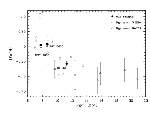
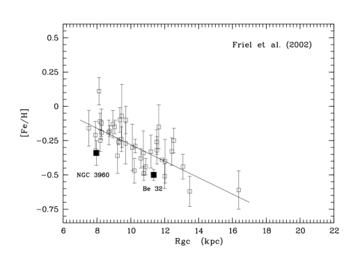
Figure 7: Radial gradient ([Fe/H] vs. Galactocentric distance) for open clusters. In the upper panel our results (filled circles) are compared to other clusters analyzed with high-resolution spectroscopy (open circles and triangles). In the lower panel the sample analyzed by Friel et al. (friel02 (2002)) is shown (filled symbols are clusters in common with the present work).

- (1) Allende Prieto, C., Asplund, M., Fabiani Bendicho, P. 2004, A&A, 423, 1109
- (2) Alonso, A., Arribas, S., & Martínez-Roger, C. 1999, A&AS, 140, 261
- (3) Asplund, M., Grevesse, N., & Sauval, A.J. 2005, in “Cosmic Abundances as Records of Stellar Evolution and Nucleosynthesis”, ASP Conference Series, eds. T.G. Barnes & F.N. Bash, Vol. 336, p.25
- (4) Bard, A., & Kock, M. 1994, A&A, 282, 1014
- (5) Bard, A., Kock, A., & Kock, M. 1991, A&A, 248, 315
- (6) Barklem, P.S., Piskunov, N., & O’Mara, B.J. 2000, A&A, 363, 1091
- (7) Beckers, J.M., Bridges, C.A., & Gilliam L.B. 1976 “A High-Resolution Spectral Atlas of the Solar Irradiance from 380 to 700 nm”, Sacramento Peak Observatories
- (8) Blackwell, D.E., Booth, A.J., Haddock, D.J., Petford, A.D., & Leggett, S. K. 1986, MNRAS, 220, 549
- (9) Boesgaard, A.M., & Friel, E.D. 1990, ApJ, 351, 467
- (10) Boesgaard, A.M., Beard, J.L., & King, J.R. 2002, AAS, 201.4401, Vol. 34, 1170
- (11) Boissier, S., & Prantzos, N. 1999, MNRAS, 307, 857
- (12) Bragaglia, A., & Tosi, M. 2006, AJ, 131, 1544
- (13) Bragaglia, A., Carretta, E., Gratton, R., et al. 2001, AJ, 121, 327
- (14) Bragaglia, A., Tosi, M., Carretta, E., et al. 2006a, MNRAS, 366, 1493 (B06a)
- (15) Bertelli, G., Bressan, A., Chiosi, C., Fagotto, F., & Nasi, E. 1994, A&AS, 106, 275
- (16) Carraro, G., Ng, Y.K., & Portinari, L. 1998, MNRAS, 296, 1045
- (17) Carraro, G., Bresolin, F., Villanova, S., et al. 2004, AJ, 128, 1676
- (18) Carretta, E., Bragaglia, A., Gratton, R., & Tosi, M. 2005, A&A, 441, 131
- (19) Carretta, E., Bragaglia, A., Gratton, R., & Tosi, M. 2004, A&A, 422, 951
- (20) Chiappini, C., Matteucci, F., & Gratton, R. 1997, ApJ, 477, 765
- (21) Corder, S., & Twarog, B.A. 2001, AJ, 122, 895
- (22) Cutri, R.M., Skrutskie, M.F., van Dyk, S., et al. 2003, VizieR On-line Data Catalog, II/246, University of Massachusetts and IPA/California Institute of Technology
- (23) Delbouille, L., Roland, G., & Neven, L. 1973, “Atlas photometrique du spectre solaire de 3000 a 10000”, Université de Liege, Institut d’Astrophysique
- (24) D’Orazi, V., Bragaglia, A., Tosi, M., & Held, E. 2006, MNRAS, 368, 471
- (25) Edvardsson, B., Andersen, J., Gustafsson, B., et al. 1993 A&AS, 102, 603
- (26) Feltzing, S., & Gustafsson, B. 1998, A&AS, 129, 237
- (27) Fitzpatrick, M.J., & Sneden, C. 1987, BAAS, 19, 1129
- (28) Friel, E.D. 1995, ARA&A, 33, 381 Friel, E.D., Janes, K.A., Tavarez, M., et al. 2002, AJ, 124, 2693
- (29) Friel, E.D. 2006, in “Chemical Abundances and Mixing in Stars in the Milky Way and its Satellites”, eds. L. Pasquini, & S. Randich, ESO Astrophysic Symposia, in press
- (30) Friel, E.D., & Janes, K.A. 1993, A&A, 267, 75
- (31) Friel, E.D., Janes, K.A., Tavarez, M., et al. 2002, AJ, 124, 2693
- (32) Friel, E.D., Jacobson, H.R., Barrett, E., et al. 2003, AJ, 126, 2372
- (33) Geisler, D., Clarià, J.J., & Minniti, D. 1992, AJ, 104, 1892
- (34) Giovagnoli, A., & Tosi, M. 1995, MNRAS, 273, 499
- (35) Gratton, R. 1988, Rome Obs. Preprint Ser. 29
- (36) Gratton, R., Carretta, E., Claudi, R., Lucatello, S., & Barbieri, M. 2003, A&A, 404, 187 (G03)
- (37) Gratton, R., Bragaglia, A., Carretta, E., & Tosi, M. 2006, ApJ, 642, 462
- (38) Gray, D.F. 1976, “Observations and analysis of stellar photospheres”, Cambridge University Press
- (39) Grevesse, N., & Sauval, A.J. 1999, A&A, 347, 348
- (40) Hartwick, F.D, & Hesser, J.E. 1973, ApJ, 183, 883
- (41) Hasegawa, T., Malasan, H.M., Kawakita, H., et al. 2004, PASJ, 56, 295
- (42) Hesser J.E., & Smith G.H. 1987, PASP, 309, 1044
- (43) Janes, K.A. 1981, AJ, 86, 1210
- (44) Kaluzny, J., & Mazur, B. 1991, Acta Astron., 41, 167
- (45) Kurucz, R.L. 1993, CD-ROM No. 9
- (46) Kurucz, R. L., Furenlid, I., Brault, J., & Testerman, L. 1984, “Solar Flux Atlas from 296 to 1300 nm”, NOAO Atlas No. 1
- (47) Lacey, C.G., & Fall, S.M. 1985, ApJ, 290, 154
- (48) Maciel, W.J., Costa, R.D.D., & Uchida, M.M.M. 2003, A&A, 397, 667
- (49) Magain, P. 1984, A&A, 134, 189
- (50) Mermilliod, J.-C., Clarià, J.J., Andersen, J., Piatti, A.E., & Mayor, M. 2001, A&A, 375, 30
- (51) Mulas, G., Modigliani, A., Porceddu, I., & Damiani, F. 2002, SPIE, 4844, 310
- (52) Noriega-Mendoza, H., & Ruelas-Mayorga, A. 1997, AJ, 113, 722
- (53) O’Brian, T.R., Wickliffe, M.E., Lawler, J.E., Whaling, J.W., & Brault, W. 1991, JOSA B, 8, 1185
- (54) Pasquali, A., & Perinotto, M. 1993, A&A, 280, 581
- (55) Pasquini, L., Avila, G., Allaert, E., et al. 2000, SPIE, 4008, 129
- (56) Paulson, D.B., Sneden, C., & Cochran, W.D. 2003, AJ, 125, 3185
- (57) Piatti A.E., Clarià J.J., & Abadi M.G. 1995, AJ, 309, 2813
- (58) Prisinzano, L., Micela, G., Sciortino, S., & Favata, F. 2004, A&A, 417, 945
- (59) Randich, S., Bragaglia, A., Pastori, L., et al. 2005, ESO Messenger, 121, 18
- (60) Randich, S., Sestito, P., Primas, F., Pasquini, L., & Pallavicini, R. 2006, A&A, 450, 557
- (61) Richtler, T., & Sagar, R. 2001, BASI, 29, 53
- (62) Rutten, R.J., & Van der Zalm, E.B.J. 1984, A&AS, 55, 171
- (63) Sandrelli, S., Bragaglia, A., Tosi, M., & Marconi, G. 1999, MNRAS, 309, 739
- (64) Schuler, S.C., King, J.R., Fischer, D.A., Soderblom, D.R., Jones, B.F. 2003, AJ, 125, 2085
- (65) Schuler, S.C., Hatzes, A.P., King, J.R., Kuerster, M., & The, L.-S. 2006, AJ, 131, 1057
- (66) Shaver, P.A., McGee, R.X., Newton, L.M., Danks, A.C., & Pottasch, S.R. 1983, MNRAS, 204, 53
- (67) Smartt, S.J., & Rollerstone, W.R.J. 1997, ApJ, 4181, L47
- (68) Smith, G. 1999, A&A, 350, 859
- (69) Sneden, C.A. 1973, ApJ, 184, 839
- (70) Tosi, M. 1988, A&A, 197, 33
- (71) Tosi, M. 1996, ASP Conf. Ser. 98, 299
- (72) Twarog, B.A., Ashman, K.M., & Anthony-Twarog, B.J. 1997, AJ, 114, 2556
- (73) Unsöld, A. 1955, “Physik der Sternatmosphären”, Springer-Verlag, Berlin
- (74) Villanova, S., Carraro, G., Bresolin, F., & Patat, F. 2005, AJ, 130, 652
- (75) Wylie, E.C., Cottrell, P.L., & Taute, K.M. 2004, MemSAIt, 75, 578
- (76) Yong, D., Carney, B.W., & de Almeida, L. 2005, AJ, 130, 597