S0 galaxies in Fornax: data and kinematics

Abstract

We have obtained long-slit spectroscopy for a sample of 9 S0 galaxies in the Fornax Cluster using the FORS2 spectrograph at the 8.2m ESO VLT. From these data, we have extracted the kinematic parameters, comprising the mean velocity, velocity dispersion and higher-moment $h_{3}$ and $h_{4}$ coefficients, as a function of position along the major axes of these galaxies. Comparison with published kinematics indicates that earlier data are often limited by their lower signal-to-noise ratio and relatively poor spectral resolution. The greater depth and higher dispersion of the new data mean that we reach well beyond the bulges of these systems, probing their disk kinematics in some detail for the first time. Qualitative inspection of the results for individual galaxies shows that they are not entirely simple systems, perhaps indicating a turbulent past. Nonetheless, we are able to derive reliable circular velocities for most of these systems, which points the way toward a study of their Tully–Fisher relation. This study, along with an analysis of the stellar populations of these systems out to large galactocentric distances, will form the bases of future papers exploiting these new high-quality data, hopefully shedding new light on the evolutionary history of these systems.

1 Introduction

One of the key areas of research in extragalactic astronomy is the study of the formation and evolution of galaxies in different environments, from the low-density field to rich clusters. Our understanding of the individual physical processes involved in the evolutionary history of galaxies, and their relative importance in each environment, is still rather poor. In this context, lenticular (S0) galaxies have a very important role. Located between elliptical and spiral galaxies in the Hubble Diagram, S0 galaxies have been a focus of debate for many years. One fundamental – and sometimes controversial – issue is whether the formation of these galaxies is more closely linked to that of ellipticals or to that of spirals.

The evolution with redshift of the morphology–density relation in clusters of galaxies (Dressler 1980; Dressler et al. 1997) implies that the relative fraction of S0 galaxies increased from $z\approx 0.5$ to the present, while the relative fraction of spirals decreased in a similar proportion. An evolutionary connection between S0s and spirals has thus been proposed, at least in cluster environments. More recent works seem to support such ideas (e.g., Fasano et al. 2000; Desai et al. 2006), although alternative views do exist (Andreon 1998). However, our understanding of the mechanisms involved in the possible morphological transformation of spirals into S0s remains poor. In addition, close similarities exist between ellipticals and S0s in their colours, stellar populations, gas content, location on the fundamental plane, etc, so the debate as to whether S0s are more closely related to spirals or ellipticals remains open.

The presence of S0s in both cluster and field environments raises the real possibility that multiple evolutionary paths exist for the formation of these systems. Indeed, a variety of mechanisms have been proposed that can, in principle, alter a galaxy’s morphology in this direction. These mechanisms include ram pressure gas stripping (Gunn & Gott 1972), harassment (Moore et al. 1998), starvation (Larson, Tinsley & Caldwell 1980; Bekki et al. 2002), unequal mass galaxy mergers (Mihos & Hernquist 1994; Bekki 1998) and galaxy-cluster interactions (Goto et al. 2003). However, it is still unclear whether any of these processes would work in practice, and, if more than one, their relative importance in different environments.

Van den Bergh (1990), analysing the Revised Shapley–Ames Catalog of Bright Galaxies (Sandage & Tammann 1987), found that the frequency distribution of the luminosity of S0s is not intermediate between E and Sa galaxies. This discontinuity could imply the existence of sub-populations amongst the S0s: bright S0s, the “real” intermediate class between E and Sa galaxies; and faint S0s, many of which could be miss-classified as faint Es if viewed close to face-on. The works of Nieto et al. (1991) and Jorgensen & Franx (1994) support this hypothesis, pointing out the similarity between disky [and thus faint (Kissler-Patig 1997)] E and S0 galaxies, based on their isophotal central shapes. Also, Graham et al. (1998), in a study of the extended stellar kinematics of elliptical galaxies in the Fornax Cluster, found that five of the galaxies are in fact rotationally supported systems, suggesting that they could be misclassified S0 galaxies.

Studies of the stellar populations in cluster galaxies (Kuntschner 2000, Smail et al. 2001) also support the idea of a dichotomy between low- and high-luminosity S0s: bright S0s are old and coeval with E galaxies, while faint members present younger central ages, indicating more recent star formation episodes. Furthermore, Poggianti et al. (2001) examined the star-formation history of early-type galaxies in the Coma Cluster, and found that $\sim 40\%$ of the S0 population seemed to have experienced a star-formation event during the last few billion years, a phenomenon which is absent in their sample of elliptical galaxies. Thus, it has been proposed that faint S0s could be the descendants of the post-starburst galaxies found in high redshift clusters. The work of Mehlert et al. (2000, 2003) in early type galaxies in the Coma Cluster confirms the dichotomy found by Poggianti et al. between old and young lenticulars; however, the high alpha-element ratios found in the latter seems to argue against the occurrence of recent star formation: the authors suggest that the strong Balmer line indices measured in apparently “young” S0s could actually be produced by unusually blue horizontal branches rather than by young stellar populations. Clearly, more work remains to be done in the study of stellar populations to interpret the physical significance of the two apparently-distinct types of S0.

The formation of lenticular galaxies has also been the subject of numerical simulations. The work of Shioya et al. (2004) on “red H$\delta$-strong” galaxies also suggests two different evolutionary paths for S0s, each one able to match different spectral features in different galaxies: a “truncation” scenario, in which the star formation is stopped and followed by passive evolution, and a “starburst” one, in which a relatively recent and short star formation event precedes the cessation of star formation. On the other hand, Christlein & Zabludoff (2004) found that simulations based on a fading stellar population could not match the observed luminosity distribution of galaxies with the larger bulge-to-total-light ratios ($B/T$) typical of S0s. They therefore advocated a “bulge enhancement” model, where disk fading is accompanied by an increase in the luminosity of the bulge; this model seems to match the observations over a wide range of $B/T$. Although this work still faces the problem of the difficulty of reliably identifying S0 galaxies, it does raise the interesting possibility that, at least in some cases, the cessation of star formation in the disk of the parent spiral galaxy could be preceded by a centrally-concentrated episode of star formation, thus enhancing the bulge luminosity. In this context, it is interesting that Moss & Whittle (2000) found spiral galaxies in clusters have more central star formation than their field counterparts.

The extended stellar kinematics of S0 galaxies have been studied mostly in conjunction with those of ellipticals, and often as one single class of objects, generically termed “early-type galaxies.” For instance, D’Onofrio et al. (1995) studied a sample of 15 early-type galaxies in the Fornax Cluster, and did not find major differences between Es and S0s other than stronger rotational support and higher projected ellipticities for the latter. In a sample of 35 E and S0 galaxies in the Coma cluster, Mehlert et al. (2000, 2003) found that elliptical galaxies have, on average, slightly higher velocity dispersions than S0s, as is also apparent from the velocity dispersion profiles presented in D’Onofrio et al. (1995). Although these differences could be real, they may also at least in part arise from the selection effects that render S0s more reliably identified when close to edge-on.

With current techniques using integral-field units and high quality spectra, it is possible to examine stellar-kinematic substructure in search of further clues as to how these systems form. The work by Emsellem et al. (2004), for example, revealed that kinematically-decoupled components, bars and misalignments between photometric and kinematic axes seems to be present in both Es and S0s. There are also instances of even more extreme kinematic substructure such as counter-rotating co-spatial stellar disks in S0s (Rubin, Graham & Kenney 1992), but these seem to be very rare (Merrifield, Fisher & Kuijken 1996). This rarity is something of a surprise, as counter-rotating gas is relatively common in S0s (Bertola, Buson & Zeilinger 1992), which led to the suggestion that it might be quite common for S0s to be enhanced by the kind of minor mergers likely responsible for this phenomenon. These observations can only be reconciled if there is some mechanism for inhibiting star formation in such counter-rotating material, but the situation is clearly quite complex.

One last approach to understanding the origins of S0 galaxies lies in their scaling relations. In particular, there are a handful of studies of the Tully–Fisher relation for S0 galaxies. Using a sample of field S0 galaxies, Neistein et al. (1999) found a much larger scatter in this relation between luminosity and rotation speed than is found in spirals. Hinz et al. (2001, 2003) found a similar result for cluster S0s. The large scatter would tend to indicate a rather stochastic history for these systems rather than any simple deterministic evolutionary path from spirals. By contrast, Mathieu, Merrifield & Kuijken (2002) selected a sample of S0s with relatively small bulges and found a Tully–Fisher relation with a small scatter but an offset to fainter luminosities relative to the spiral relation, suggesting a relatively simple fading of spirals into S0s for this sub-sample of systems.

The above discussion illustrates the wide range of techniques that have been applied to trying to understand the nature of S0s, and the rather contradictory results that have emerged. There are certainly indications of a dichotomy between faint and bright S0s, but it is still unclear which observables best characterize this distinction, and how those observables might translate into differences in the evolutionary history of the two types. Much of the difficulty arises from the heterogeneous nature of the data that have been used in these studies. In some cases, the data come from objects in a range of ill-defined differing environments, while in others the issues are more to do with the varying quality of the observations.

To address these issues, we have obtained very high signal-to-noise ratio long-slit spectroscopy of 9 S0 galaxies in the Fornax Cluster. The data are uniform in quality and probe in detail a single environment, removing these variables from the problem. However, the sample does include both faint and bright examples of S0s, allowing us to investigate whether there are systematic differences between these systems in anything other than luminosity, and hence address the question of whether they formed in different ways. In this paper, we present the details of the sample, the observations, the data reduction, the resulting kinematics, and a qualitative look at the results. In subsequent papers, we will delve deeper into the quantitative information that these data provide, looking at their Tully–Fisher relation and the nature of their stellar populations out to large radii.

The layout of this paper is as follows: Section 2 describes the sample and observations; Section 3 explains the basic data reduction; Section 4 describes the extraction of the kinematics; Section 5 presents the resulting kinematics and comparison to previous data; Section 6 extracts the rotation curves from these data; and Section 7 contains a summary.

2 The sample and observations

The sample was selected from galaxies in the Fornax Cluster classified as S0s by the NASA/IPAC Extragalactic Database. They were selected to span a wide range of luminosities ($-22.3<M_{B}<-17.3$), and to be sufficiently inclined to measure rotations along their major axes. The basic properties of the resulting sample of S0s are presented in Table 1.

The necessary observations of the major axes of these galaxies were made in service mode between 2002 October 2 and 2003 February 24 at the 8.2m Antu/VLT using the FORS2 instrument in long-slit spectroscopy mode; exposure times and dates are provided in Table 1. Spectrophotometric standard stars were observed each night, and we also obtained spectra of stars with a range of spectral classes to act as velocity templates in the kinematic analysis; these objects are listed in Table 2. During the observations, the seeing varied from 0.75 to 1.48 arcsec FWHM, which is more than adequate for the study of these large objects.

The detector in FORS2 comprises two 2k$\times$4k MIT CCDs, with a pixel size of $15\times 15\mu{\rm m}^{2}$. The standard resolution collimator and the unbinned readout mode were used, yielding a scale of $0.125^{\prime\prime}$/pixel. The spectrograph slit was set to $0.5^{\prime\prime}$ wide and covered $6.8^{\prime}$ in length. The GRIS$1400V+18$ grism was used, providing a dispersion of $0.318$Å/pixel and covering the 4560Å $\leq\lambda\leq 5860$Å wavelength range. This set-up provided a spectral resolution, as measured from the FWHM of the arc lines, of $\approx 4$ pixels (or 1.12 Å), which translates into a velocity resolution of $73.3\,$km s^-1 FWHM (or $31.0\,$km s^-1 in terms of the velocity dispersion). The CCD was read out at $200\,$kHz, which is twice the normal speed used for spectroscopy. The high readout speed was the only one available for unbinned readout of the CCD.

Table 1: Sample of S0 galaxies in Fornax.

Name	RA	DEC	$B_{\rm T}^{*}$	Diameter∗	Exp. Time	Date
				[′]	[sec]
NGC 1316	03 22 41	$-$37 12 30	9.40	11.0	$3\times 1200$	13 Oct 2002
NGC 1380	03 36 27	$-$34 58 34	10.9	4.8	$2\times 1200$	24 Feb 2003
NGC 1381	03 36 31	$-$35 17 43	12.4	2.7	$2\times 1600$	24 Feb 2003
IC 1963	03 35 30	$-$34 26 51	12.9	2.6	$2\times 1600$	31 Jan 2003
NGC 1375	03 35 16	$-$35 15 56	13.2	2.2	$2\times 1800$	28 Dec 2002
NGC 1380A	03 36 47	$-$34 44 23	13.3	2.4	$2\times 1700$	28 Dec 2002
ESO 358$-$G006	03 27 18	$-$34 31 35	13.9	1.2	$2\times 2400$	14 Oct 2002
ESO 358$-$G059	03 45 03	$-$35 58 22	14.0	1.0	$1\times 2550$	8 Feb 2003
ESO 359$-$G002	03 50 36	$-$35 54 34	14.2	1.3	$1\times 2250$	26 Nov 2002

^∗ From RC3, de Vaucouleurs et al. (1991).

3 Data Reduction

The standard data reduction process was carried out using IRAF (Tody 1986, 1993). Bias subtraction, flat-fielding and cosmic ray removal were applied to all science and calibration images. Bad pixel masks were created by dividing two flatfield images of different exposure times, and the bad pixel values were interpolated. When more than one exposure was obtained for each galaxy (see Table 1), the individual spectral images were combined to maximise the signal-to-noise ratio (S/N). During the combination process the position of the galaxy spectrum and the locations and widths of several sky lines were checked; the match between the different exposures for each galaxy was found to be excellent, so no further alignment was necessary.

After tracing the arc lines of the He–Ne lamp, a 2D correction was applied to all the spectra in order to remove the geometric distortions due to the instrument optics and CCD flatness issues. The wavelength calibration was applied in the same step. The residuals of the wavelength fits were typically 0.1–0.2Å.

Next, we subtracted the night sky spectrum using the IRAF task background. Potentially, residuals and uncertainties from sky subtraction could bias the kinematic and line strength measurements that we will make from these data, so we have looked quite closely at how this step is implemented. Given the large spatial coverage of the data, there are sizeable regions that are free of galaxy light from which we can define a sky spectrum, and we found that the resulting sky-subtracted galaxy spectrum was almost completely insensitive to how the sky region was chosen. We have therefore opted for the simplest choice of selecting sky regions, typically 100 pixels wide, on each side of the galaxy and as far from it as possible within the confines of the slit. The only exception is the case of NGC 1316, the largest and brightest galaxy, where only one sky region was used because the galaxy centre was placed close to one end of the slit in order to maximise the spatial coverage. Contamination by scattered light was not found to be a significant issue: in all cases, there were no nearby bright sources, and the relatively low surface brightnesses of the systems reduces the likelihood of misplaced light from the galaxies themselves.

A periodic, square wave noise pattern or ‘hum’ was found to be present along the dispersion direction in all the spectra. The amplitude of this hum varied from 3 to 6 counts, and its frequency, 0.077 cycles/pixel ($15\,$kHz), was reasonably constant, with small deviations due mainly to previous data processing. Because this pattern could partially mask the spectral features at low S/N, we subtracted it using a Fourier technique (Brown 2001). Ideally, one would apply this technique to the raw data frames, but its low level meant that it could only be reliable identified and removed after processing to subtract the sky. In practice, inspection of the resulting cleaned images showed that this processing had no adverse impact on our ability to remove this source of systematic noise.

To correct by the effect of atmospheric extinction, we used the IRAF task setairmass to define the effective airmass for each spectrum. Then, we applied the extinction correction (task calibrate) using the appropriate atmospheric extinction table. The spectra were subsequently flux calibrated using the set of spectrophotometric standard stars listed in Table 2, which allowed us to transform the observed counts into relative spectral fluxes as a function of wavelength. The sensitivity functions as derived from the different stars varied by typically $\sim 1$%, reaching $\sim 3$% towards the edges of the wavelength range, so we created a single function from all of them and can be reasonably confident that the resulting internal relative flux calibration is good to $\sim 1\%$.

This analysis was applied both to the galaxy spectra and to the spectra of the 10 template stars (listed in Table 2), which will be used to model the spectra of the galaxies during the extraction of the kinematics.

Table 2: Spectrophotometric (S) and Template (T) Stars.

Name	T/S	Spectral Class
BD-01-0306	T	G1 V
HD1461	T	G0 IV
HD7565	T	K2 III-IV
HD16784	T	G0 V
HD18234	T	K0
HD19170	T	K2
HD21197	T	K5 V
HD23261	T	G5
HD36395	T	M1.5 V
HD61606	T	K2 V
LTT1020	S	–
LTT1788	S	–
LTT3218	S	–
HZ4	S	–
GD71	S	–
Feige67	S	–

The calibrated two-dimensional galaxy spectra were binned along the spatial direction so as to generate one-dimensional spectra from different radii with comparable S/Ns. We started at the centre of the each galaxy using bins with a S/N per Ångstrom of 53 (or 30 per pixel). When we reached the outer parts, where no more bins with that S/N ratio could be built, we reduced the S/N of each bin to 30 per Ångstrom, then to 15, and finally to 10. The data were also re-binned on to a logarithmic wavelength scale in the dispersion direction to enable the kinematic measurements.

4 Extraction of the kinematics

In the present study, the kinematic properties of the galaxies were derived using the Penalised Pixel Fitting method (pPXF, Cappellari & Emsellem 2004), which is a parametric technique based on maximum penalised likelihood. Since the resulting kinematic parameters are so central to this work, we first describe the workings of this method as they apply to the current data set, and the tests that we undertook to check the reliability of the resulting parameters.

The parametric method used by pPXF models the line-of-sight velocity distribution (LOSVD) as a Gaussian plus a series of Gauss-Hermite polynomials. The fits return the mean line-of-sight velocity, $V_{\rm LOS}$, and the velocity dispersion, $\sigma$, from the Gaussian, together with the $h_{3}$ and $h_{4}$ coefficients from the polynomials. These two coefficients are related, respectively, to the skewness and the kurtosis of the LOSVD, which are higher moments associated with the asymmetric and symmetric departures of the LOSVD from a Gaussian.

This software works in pixel space, finding the combination of template spectra which, convolved with an appropriate LOSVD, best reproduces the galaxy spectrum in each bin. A subroutine of the program fits the continuum, using Legendre polynomials of order 4 (in this case), and divides the spectra by the fit to remove any possible low-frequency mismatches between the galaxy spectra and the model. The method carries out a pixel-by-pixel minimisation of the residuals (quantified by $\chi^{2}$), adding an adjustable penalty term to the $\chi^{2}$ to bias the resulting LOSVD towards a Gaussian shape when the higher moments $h_{3}$ and $h_{4}$ are unconstrained by the data. Thus, a deviation $D$ of the LOSVD from a Gaussian shape will be accepted as an improvement of the fit only if it is able to decrease the residuals by an amount

$$\chi^{2}_{p}=\chi^{2}(1+\lambda^{2}\cdot D^{2}).$$ (1)

The $\lambda$ parameter defines the threshold between a deviation considered as an improvement of the pure Gaussian fit, and one considered as due to noise, and thus rejected. As Cappellari & Emsellem (2004) suggest, the value of $\lambda$ has to be determined for each particular dataset because the ability of the software to find the correct LOSVD parameters (especially the higher moments) will depend critically on the S/N of the data and other properties of the particular spectra such as the spectral range covered. To estimate the optimum parameter for our study, we performed Monte-Carlo simulations in which we convolved the template spectra with a LOSVD whose shape was specified by model parameters $V_{\rm in}$, $h_{3\rm in}$ and $h_{4\rm in}$, and whose width was allowed to vary such that $0<\sigma_{\rm in}<250\,$km s^-1. These spectra, degraded to the S/N of the various one-dimensional galaxy spectra, were then passed through the pPXF software to recover estimates for the parameters, $V_{\rm out}$, $\sigma_{\rm out}$, $h_{3\rm out}$ and $h_{4\rm out}$. An example of one such run is presented in Figure 1. After extensive testing using a variety of input parameters and S/N, we found that $\lambda=0.3$ provided an optimum value for the spectra in the current dataset, yielding values that minimized both errors and bias in the results.

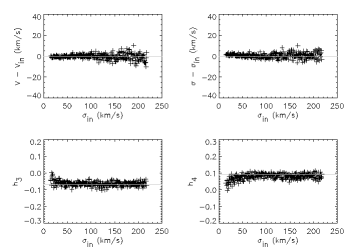
Figure 1: Sample 1000 pPXF simulations carried out in order to find the optimum value of the $\lambda$ parameter for this dataset. In this particular case, the simulated spectra have S/N $=53$ and $\lambda$ has been set to 0.3. The model LOSVD has $V_{\rm in}=0$, $h_{3\rm in}=-0.07$, $h_{4\rm in}=0.09$ and the derived values of $V_{\rm out}$, $h_{3\rm out}$ and $h_{4\rm out}$ are shown for different values of $\sigma_{\rm in}$.

As is apparent from Figure 1, even at this fairly modest value for the $\lambda$ parameter, a degree of bias appears in the answers at low dispersion, particularly in the derived values of $\sigma$ and $h_{4}$. This kind of bias, particularly prevalent in such even moments, is a well-known phenomenon (e.g. Cappellari & Emsellem 2004). Clearly, we must understand and possibly correct for this effect before interpreting the calculated parameters, so we have performed a range of tests using our adopted value of $\lambda$ but allowing other parameters to vary. The conclusion of this study is that the bias in $\sigma$ is small but well-defined at a maximum level of $\pm 2$-$3\,$km s^-1; we corrected the results for this bias, but it makes no substantive difference. The case for $h_{4}$ is a little more disturbing, as this parameter, particularly in galaxies with low values of $\sigma$, can suffer significant bias, amounting to offsets as high as 0.4 in the most extreme cases. The uncertain nature of this bias means that we have not corrected for it explicitly in our final derived value, but we would caution against interpreting the $h_{4}$ values as too precise, particularly from spectra where S/N is low and where $\sigma$ is small. Nonetheless, this study does demonstrate that the principal parameters of interest, $V_{\rm LOS}$ and $\sigma$, are robustly extracted from spectra of the quality that we present here, irrespective of the detailed shape of the LOSVD as specified by $h_{3}$ and $h_{4}$.

To estimate the errors on the derived parameters for each one-dimensional galaxy spectrum, we ran a further series of Monte Carlo simulations. We modelled each such spectrum using the corresponding best combination of template stars, broadened by the best-fit LOSVD, and degraded to the S/N of the galaxy data. These model spectra were then passed through the pPXF software to measure the distribution of the derived parameters, and hence a measure of the uncertainty in a single spectrum. The dispersion in the parameters derived in each Monte Carlo simulation is quoted as the error bar on the corresponding parameter derived for the real galaxy spectrum.

Before we can present the final data set of kinematic parameters versus distance along the major axes for these S0 galaxies, the only remaining issue is to define the zero-points of velocity and position for each galaxy. The velocity zero-point was simply set to the median value of $V_{\rm LOS}$ determined along the slit for each galaxy. For the spatial zero-point – the galaxy’s centre – the simplest definition would just be the point along the slit that admitted the greatest amount of light. However, this definition could well pick up on an off-centre localized feature that would then distort the over-all kinematic structure of each galaxy that is the primary goal of this study. Instead, we adopted as the spatial origin the position along the slit that renders the plot of $V_{\rm LOS}$ versus radius as close to anti-symmetric as possible. The only case where this method was not applied was NGC 1316; the large size of this system meant that we placed the slit primarily to cover only one side of the galaxy, so we could not subtract the median velocity along the slit nor match up the two sides of the rotation curve to find the kinematic centre. For this galaxy, we used the point along the slit at which we derived the largest value of $\sigma$ to define the spatial location of the galaxy’s centre, and then used the value of $V_{\rm LOS}$ at this point to specify the galaxy’s systemic velocity.

5 Results and comparisons

The values for the kinematic parameters $V_{\rm LOS}$, $\sigma$, $h_{3}$ and $h_{4}$ versus radius, as derived using the analysis set out in Section 4, are presented in Appendix A.

A number of these galaxies have been studied previously with lower quality spectra or less sophisticated spectral analyses, so as well as presenting our own results we will also compare the data to these published results. The most extensive study for comparison is that of D’Onofrio et al. (1995), who obtained major-axis kinematics ($V_{\rm LOS}$ and $\sigma$) for six galaxies in common with the current sample. One complication in comparing their data with the new observations is that they presented the kinematics folded about the centre of each galaxy, leading to an ambiguity in the actual spatial location of each measurement. We therefore cannot match up individual features that occur on one side of a galaxy, but can use these data to examine the overall profile. The other limitation of their data was its relatively low spectral resolution ($\sim 60\,{\rm km}\,{\rm s}^{-1}$ in velocity dispersion), which, as we will see, introduces a significant bias into the kinematics. Further long-slit data for single galaxies in the current sample can be found in Graham et al. (1998) and Longhetti et al. (1998), so we also include these data in our comparison. There are also a number of measurements of the central velocity dispersion that provide a single comparison point. Kuntschner (2000) obtained central dispersions for all the galaxies in this sample, although he warns that the relatively low spectral resolution of his data, corresponding to a velocity dispersion of $\sim 50\,{\rm km}\,{\rm s}^{-1}$, mean that the measurements should only provide a rough guide for the fainter galaxies. Further measurements can be found in the compilation of Bernardi et al. (2002), although the variety of sources from which these data were drawn mean that their reliability is less assured than in the other measurements.

5.1 Results for individual galaxies

In the following paragraphs we give a brief description of the observed kinematics for each individual galaxy in the sample. We discuss these result and compare them with the previous studies described above.

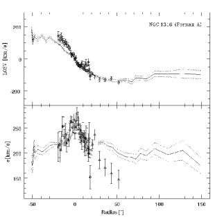
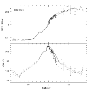
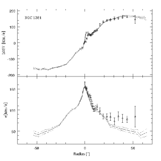
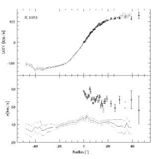
Figure 2: Comparison between the new results for mean velocity, $V_{\rm LOS}$, and velocity dispersion, $\sigma$, and kinematics from the literature for NGC 1316, NGC 1380, NGC 1381 and IC 1963. The new results are shown as a continuous line with $1\sigma$ errors as short dashed lines. The D’Onofrio et al. (1995) data are shown as triangles, the Longhetti et al. (1998) data are shown as stars, and the Graham et al. (1998) data are shown as squares. Horizontal dashed lines in the velocity dispersion plots indicate the resolution limit of the archival data.

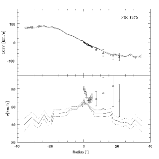
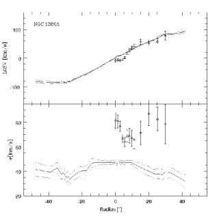
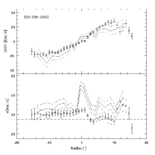
Figure 3: As for Figure 2, for NGC 1375, NGC 1380A and ESO 359-G002

5.1.1 NGC 1316 (FORNAX A)

For this well-known merger remnant, Figure 2 reveals generally good agreement with the published results, although the new data reach to very much larger radii. The new data indicate a rather higher dispersion than the points at the largest radii of the previous measurements, but since these points were derived from the lowest S/N data in the older observations, the conflict is probably not significant. The more extended velocity dispersion profile from the new data for the first time reveals a seemingly-distinct feature of enhanced dispersion within the central $15\,{\rm arcsec}$. In this galaxy, as might be expected in a merger, random motions dominate out to large radii in the new data, bringing into question whether this galaxy should really be classified as an S0 system.

5.1.2 NGC 1380

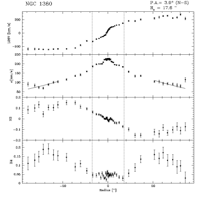
Figure 6: The major-axis kinematics of NGC 1380.

Figure 2 shows that the new data agree extremely well with the previous observations, but with much improved error bounds. The new data with their smaller errors and unfolded presentation give some indication of localized substructure that differs between the two sides of the galaxy. An enhancement in velocity dispersion within the central $\sim 7\,{\rm arcsec}$, first suggested by D’Onofrio et al. (1995), is strongly confirmed with the new data. It is also notable from Figure 6 that this region also shows structure in the $h_{3}$ skewness measure, indicative of a distinct kinematic component. Interestingly, this feature coincides with photometric evidence for a distinct component which comprises a strong variation in isophotal ellipticity and position angle (Caon et al. 1994).

5.1.3 NGC 1381

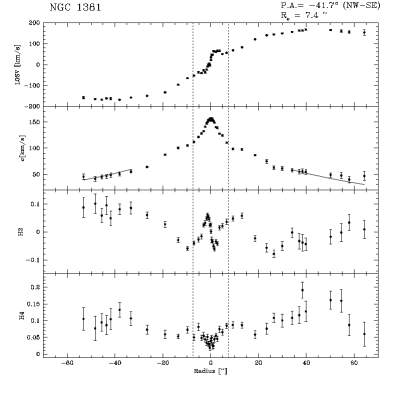
Figure 7: The major-axis kinematics of NGC 1381.

Figure 2 reveals a distinctive feature in this galaxy’s rotational motion which was not apparent in the previous data. There is a correspondingly very strong signal in the $h_{3}$ profile shown in Figure 7. Such kinematic features are characteristic of a bar viewed edge-on (Bureau & Athanassoula 2005), so we would seem to have identified this edge-on galaxy, previously designated as unbarred, as a barred system. The new velocity dispersion profile diverges at large radii from the D’Onofrio et al. (1995) data, but this would seem to be because the latter has been artificially enhanced in regions where the dispersion approaches the resolution limit of the older data.

5.1.4 IC 1963

Figure 2 shows very good agreement between new measurements of mean streaming velocity and those in D’Onofrio et al. (1995) for this rather nondescript S0 system. The velocity dispersion measurements do not agree at all well, but once again this conflict can be attributed to the inadequate spectral resolution of the older data.

5.1.5 NGC 1375

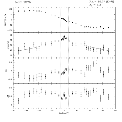
Figure 9: The major-axis kinematics of NGC 1375.

Once again, Figure 3 shows that the measured rotational motion for this galaxy agrees well with previous data, while the disagreement with earlier velocity dispersion data seems to arise from the limited spectral resolution of the older data. Support for this interpretation of the inconsistency comes from Kuntschner’s (2000) value for the central dispersion of $56\pm 10\,$km s^-1, in agreement with the new data. A further issue with the earlier analysis is revealed by Figure 9, as the structure in $h_{3}$ and $h_{4}$ at small radii would indicate that there is more information in these dynamics than would be revealed by the earlier Gaussian fit. Once again, this structure indicates the presence of a distinct kinematic component such as a bar. Photometric support for this conclusion comes from the work by Lorenz et al. (1993), who found that NGC 1375 possesses a complex structure characterised by boxy isophotes within a radius of $15\,{\rm arcsec}$; such boxy isophotes are often associated with the kinematic signature of an edge-on bar (Kuijken & Merrifield 1995).

5.1.6 NGC 1380A

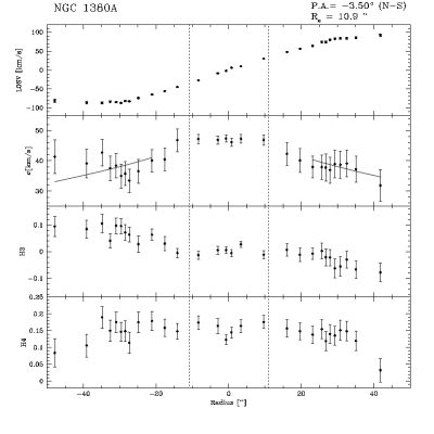
Figure 10: The major-axis kinematics of NGC 1380A.

The well-constrained measurements of rotational motion for this galaxy are fairly featureless, and, as Figure 3 shows, do not reproduce the rather strange profile found by D’Onofrio et al. (1995). The similar absence of peculiarities in the $h_{3}$ and $h_{4}$ profiles shown in Figure 10 suggest that the velocity structure in this galaxy is quite simple, so the smooth mean velocity curve is not unexpected. Once again, the new measurements of velocity dispersion lie systematically well below those in D’Onofrio et al. (1995), presumably due to the spectral resolution of the latter; Kuntschner’s (2000) published central dispersion of $55\pm 9\,{\rm km}\,{\rm s}^{-1}$ fits rather better with the new measurements, but may also be running into resolution issues.

5.1.7 ESO 359-G002

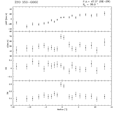
Figure 11: The major-axis kinematics of ESO 359-G002.

As Figure 3 shows, this fainter lenticular galaxy has a slowly rising mean velocity curve, in good agreement with the previous data from Graham et al. (1998) and despite being below our estimated spectral resolution. The previous velocity dispersion measurements are in reasonable agreement with the new data, but seem to lie systematically lower. In particular, the sharp central peak in velocity dispersion, which is accompanies by a similar structure in $h_{4}$ (see Figure 11), was not seen in the earlier data. In this case both, the velocity curve and the dispersion profile should be viewed with some caution.

5.1.8 ESO 358-G006

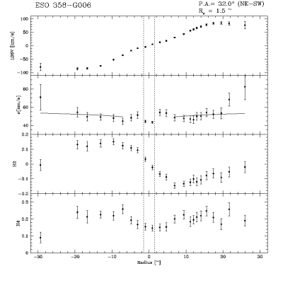
Figure 12: The major-axis kinematics of ESO 358-G006.

There are no previous studies of the extended kinematics for this faint galaxy. Figure 12 reveals generic featureless rotational motions that rise to a plateau at large radii, and a rather strange velocity dispersion profile with a slight central depression and a hint of a rising profile at large radii. The existing values for the central velocity dispersion of $58\pm 8\,{\rm km}\,{\rm s}^{-1}$ from Kuntschner (2000) and $46\pm 3\,{\rm km}\,{\rm s}^{-1}$ (Bernadi et al. 2002) are in accord with the new dispersion measurements.

5.1.9 ESO 358-G059

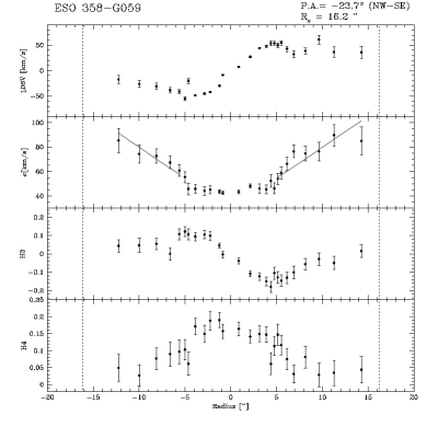
Figure 13: The major-axis kinematics of ESO 358-G059.

The extended kinematics of this faint galaxy have not previously been studied. Figure 13 shows the rather strange kinematics for this system. It has a relatively well-behaved mean velocity profile that rises to an amplitude of $\sim 50\,{\rm km}\,{\rm s}^{-1}$ at $\sim 5\,{\rm arcsec}$, then declines slightly. The dispersion profile is remarkably flat in the region where the rotation increases, then starts to rise when the rotational velocities decline. The published values for the central velocity dispersion, $54\ \pm 9{\rm km}\,{\rm s}^{-1}$ (Kuntschner 2000) and $46\pm 3\,{\rm km}\,{\rm s}^{-1}$ (Bernadi et al. 2002), are in reasonable agreement with the new data. One possible explanation for the enhanced dispersion and depressed rotation at larger radii would be the presence of a counter-rotating stellar disk (Rubin et al. 1992), but for such a faint galaxy we clearly do not have data of sufficient quality to test this hypothesis rigorously.

6 Circular velocity calculation

In order to go beyond the kinematic measurements of Section 5 to place these observations in their astrophysical context, we have to translate them into the related intrinsic dynamical properties of the galaxies. In particular, since we ultimately want to explore the Tully–Fisher relation for these galaxies, we need to derive the circular velocity as a function of radius, $V_{\rm C}(R)$. Although this quantity is clearly connected to the observed mean velocity profile, $V_{\rm LOS}(R)$, the transformation from one to the other is not trivial, so we describe the procedure we have adopted in some detail.

The first ingredient we need is the inclination, $i$, of the galaxy to the line of sight, in order to determine the fraction of rotational motion that will have been projected into the observed line-of-sight mean velocity. In principle, the inclination can be estimated by simply measuring the flattening of isophotes at large radii, but this approach is not advisable as it uses only the lowest S/N photometry. Instead, we have carried out a full two-dimensional fit to images of the galaxies using the GIM2D software (Simard et al. 2002). We have applied this software to the publicly-available 2MASS $K$-band images of the objects in our sample (Jarrett et al. 2003). The uniform quality of these data means that we can study all of the galaxies in a consistent manner, and the use of infrared light means that we are tracing the bulk of the population in these systems, avoiding any problems that might arise from localized star formation or dust obscuration. In addition to obtaining a best estimate for the galaxies’ inclinations, this analysis also returns estimates for the parameters of a disk-plus-bulge model, including a bulge effective radius, $R_{\rm e}$, and a disk scalelength, $R_{\rm exp}$. As we will see below, these photometric parameters are also useful in determining the properties of the rotation curve, so their values are presented in Table 3.

Table 3: Structural and other important parameters of S0 galaxies in the Fornax Cluster.

Name	$i$	$B/T$	$R_{\rm e}$	$R_{\rm exp}$	Sèrsic	$R_{\rm LIM}$	$R_{\rm out}$	$V_{\rm max}$	$M_{B}$
	[o]		[”]	[”]	$n$	[”]	[”] {$[R_{e}]$}	[km s-1]
(1)	(2)	(3)	(4)	(5)	(6)	(7)	(8)	(9)	(10)
NGC 1316	$43.2^{\phantom{1}43.8}_{\phantom{1}42.4}$	$0.58^{\phantom{1}0.62}_{\phantom{1}0.47}$	$36.0^{\phantom{1}41.7}_{\phantom{1}24.8}$	$49.4^{\phantom{1}52.7}_{\phantom{1}47.2}$	$2.9^{\phantom{1}3.2}_{\phantom{1}2.3}$	–	148.5 {4.1}	–	-22.3 (0.1)
NGC 1380	$66.9^{\phantom{1}67.5}_{\phantom{1}66.5}$	$0.58^{\phantom{1}0.59}_{\phantom{1}0.57}$	$17.6^{\phantom{1}18.0}_{\phantom{1}17.3}$	$36.3^{\phantom{1}37.3}_{\phantom{1}35.9}$	$3.3^{\phantom{1}3.4}_{\phantom{1}3.3}$	35.7	88.6 {5.0}	309.6 (26.6)	-20.6 (0.1)
NGC 1381	$82.5^{\phantom{1}82.9}_{\phantom{1}82.2}$	$0.57^{\phantom{1}0.58}_{\phantom{1}0.55}$	$7.4^{\phantom{1}7.7}_{\phantom{1}7.3}$	$20.8^{\phantom{1}21.6}_{\phantom{1}20.3}$	$3.1^{\phantom{1}3.2}_{\phantom{1}3.0}$	35.2	64.2 {8.7}	278.8 (32.4)	-19.0 (0.1)
IC 1963	$84.6^{\phantom{1}84.7}_{\phantom{1}84.3}$	$0.39^{\phantom{1}0.42}_{\phantom{1}0.36}$	$22.6^{\phantom{1}24.9}_{\phantom{1}21.2}$	$15.8^{\phantom{1}16.1}_{\phantom{1}15.5}$	$3.6^{\phantom{1}3.7}_{\phantom{1}3.5}$	5.5	47.8 {2.1}	164.7 (16.8)	-18.5 (0.1)
NGC 1375	$67.5^{\phantom{1}68.3}_{\phantom{1}66.3}$	$0.19^{\phantom{1}0.21}_{\phantom{1}0.17}$	$3.2^{\phantom{1}3.4}_{\phantom{1}2.9}$	$14.8^{\phantom{1}15.2}_{\phantom{1}14.0}$	$2.2^{\phantom{1}2.3}_{\phantom{1}2.1}$	10.7	35.9 {11.2}	113.4 (19.6)	-18.2 (0.2)
NGC 1380A	$78.1^{\phantom{1}78.8}_{\phantom{1}77.4}$	$0.18^{\phantom{1}0.24}_{\phantom{1}0.14}$	$10.9^{\phantom{1}14.5}_{\phantom{1}8.1}$	$19.8^{\phantom{1}20.4}_{\phantom{1}19.2}$	$3.7^{\phantom{1}3.8}_{\phantom{1}3.6}$	5.5	47.9 {4.4}	119.7 (3.0)	-18.1 (0.2)
ESO 358$-$G006	$65.9^{\phantom{1}67.2}_{\phantom{1}64.8}$	$0.02^{\phantom{1}0.04}_{\phantom{1}0.01}$	$1.5^{\phantom{1}2.9}_{\phantom{1}0.2}$	$9.2^{\phantom{1}9.6}_{\phantom{1}8.8}$	$3.0^{\phantom{1}3.3}_{\phantom{1}2.7}$	0.00627	29.4 {19.6}	155.8: (26.0)	-17.5 (0.2)
ESO 358$-$G059	$61.9^{\phantom{1}63.9}_{\phantom{1}59.8}$	$0.72^{\phantom{1}0.76}_{\phantom{1}0.65}$	$16.2^{\phantom{1}18.4}_{\phantom{1}14.7}$	$2.3^{\phantom{1}2.5}_{\phantom{1}2.2}$	$2.0^{\phantom{1}2.2}_{\phantom{1}1.6}$	–	14.2 {0.9}	108.5: (53.8)	-17.4 (0.2)
ESO 359$-$G002	$49.4^{\phantom{1}51.7}_{\phantom{1}47.2}$	$0.070^{\phantom{1}0.14}_{\phantom{1}0.029}$	$36.0^{\phantom{1}41.7}_{\phantom{1}24.8}$	$7.8^{\phantom{1}8.2}_{\phantom{1}7.4}$	$3.1^{\phantom{1}3.4}_{\phantom{1}2.9}$	0.4	13.9 {0.4}	–	-17.3 (0.2)

Note: For all pertinent calculations, $H_{0}=70\,$km s${}^{-1}\,$Mpc^-1. From (2) to (6), $99\%$ confidence intervals are presented; from (9) to (10), $1\,\sigma$ errors between “()”. Col (2), inclination angle with respect to the line-of-sight; col (3), bulge to total fraction; col (4), effective radius; col (5), exponential disk scale length; col (6), Sérsic index; col (7), minimum radius where the “projected velocities correction” is applied; col (8), distance of the outermost bin in arc-seconds and in units of the effective radius; col (9), maximum circular velocity, values followed by ’:’ should be taken as an upper limit only; col (10), absolute magnitude in B-band, assuming a redshift of 0.0043 for the cluster, according to Madore et al. (1999).

To convert line-of-sight velocities into rotational motions, we follow the approach developed by Neistein et al. (1999, hereafter N99). First of all, allowance has to be made for the extra degree of “roundness” contributed by the fact that the disks of S0s are not infinitely thin; as in N99, we assume that all galaxies would have an edge-on axis ratio of 0.22, although this assumption turns out not to be critical to the results.

The second major effect that must be corrected for is that arising from projection along the line-of-sight. Although stars close to the minimum radius along a line through a highly-inclined disk will have most of their rotational velocity projected along the line of sight, those further from the centre of the galaxy will have most of their motion transverse to the line of sight, so their measured component of velocity will be small. This tail of low-velocity stars means that the measured line-of-sight mean velocity will lie systematically below the rotational velocity of the stars. We have therefore applied a correction for this effect, which is described in Merrett et al. (2006). This technique can only be reliably applied in regions where the disk dominates the light, so we have used the photometric parameters derived above to ascertain the minimum radius, $R_{\rm LIM}$, at which this correction can be made; the values for $R_{\rm LIM}$ are given in Table 3. Clearly, if $R_{\rm LIM}$ can’t be estimated within the radius to which we have obtained data, then we will not be able to apply this correction, so will be unable to obtain a reliable rotation curve. Where it can be applied, this correction amounts to $\sim 20$%; although it is clearly significant, it is still sufficiently small that its exact value is not critical.

The last correction that we must apply is the difference between mean streaming velocity, $V_{\phi}$, and circular rotation speed that arises because the stars have a random component to their motions as well as a rotational motion. This “asymmetric drift” can be corrected using the appropriate Jeans equation (Binney & Tremaine 1987), and here we follow the N99 implementation of this correction, by which

$$V_{\rm c}^{2}=V_{\phi}^{2}+\sigma_{\rm fit}^{2}\left(2\frac{R}{R_{\rm exp}}-1\right),$$ (2)

where $\sigma_{\rm fit}$ is the velocity dispersion at radius $R$ determined from a fit to the velocity dispersion profile using a low-order polynomial (see Appendix A).

Strictly speaking, this low-order correction is only valid for rather cold disks with $V_{\phi}\gg\sigma_{\rm fit}$. Some experimenting with simulated data revealed that the corrections remained fairly reliable for any galaxy with $V_{\phi}/\sigma_{\rm fit}>2$, but that artifacts from the correction would begin to appear in the rotation curve below this limit. We can meet this requirement for five of the sample galaxies, but for two (ESO 356-G006 and ESO 358-G059), we must relax the limit to $V_{\phi}/\sigma_{\rm fit}>1$. In these cases, the asymmetric drift correction of equation 2 tends to be too large, so the resulting rotation velocities should strictly be taken as only an upper limit. In two cases (NGC 1316 and ESO 359-G002), random motions dominate at all radii, so this correction cannot even be attempted. In consequence, these two galaxies have to be excluded from subsequent analysis.

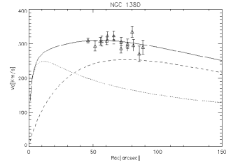
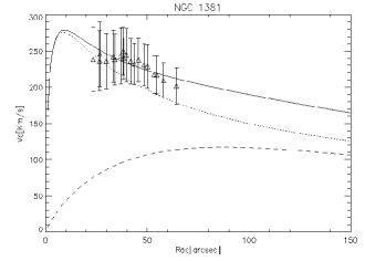
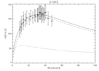
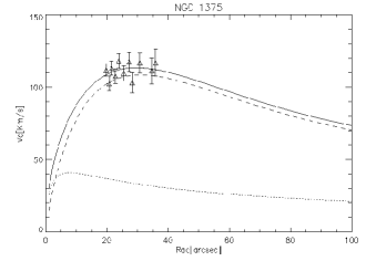
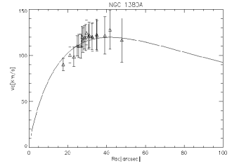
Figure 4: Derived circular velocity as function of radius and the corresponding best-fit models for Fornax Cluster S0 galaxies. The dotted line shows the bulge contribution, the dashed line shows the disk contribution, and the solid line shows the quadrature-summed total. For NGC 1380A a pure disk model gives the best fit.

After carrying out the above procedures, we can convert the measured mean line-of-sight velocity data points into discrete estimates of the local circular speed at the corresponding radii. These estimates have two limitations: first, each point will have a significant error bar from all the propagated uncertainties; and second, the data will lie over only a limited range in radii since the rotation velocities cannot be determined in this way at small radii where random motions dominate, and the galaxies become too faint at large radii to have their kinematics measured. We therefore cannot simply read off dynamical parameters such as the maximum velocity, $V_{\rm max}$, from these data. Instead, we effectively interpolate and extrapolate the limited data by modelling the contributions to the rotation curve by disk and bulge. Using the photometric parameters derived above, we model the disk component of the rotation curve using the formula for a pure exponential,

$$V_{c}^{2}(R)=4\pi G\Sigma_{0}R_{exp}y^{2}[I_{0}(y)K_{0}(y)-I_{1}(y)K_{1}(y)],$$ (3)

where G is the gravitational constant, $\Sigma_{0}$ is the central surface density, $I_{0},K_{0},I_{1}$ and $K_{1}$ are modified Bessel functions, and $y=R/R_{\rm exp}$ (Freeman 1970). For the bulge, we use the rotation curve of Hernquist (1990),

$$V_{c}^{2}(R)=\frac{GM_{bulge}}{R}\frac{R^{2}}{(R+a)^{2}},$$ (4)

where $M_{\rm bulge}$ is the mass of this component, and the scalelength $a$ can be approximately related to $R_{\rm e}$ by $a/R_{\rm e}=1.82$. The normalizations of these two components (effectively, the mass-to-light ratios of the photometric components) were then varied such that their sum produced the best fit to the circular speed data over the range that it is available. The result of this process is presented in Figure 4; we have not attempted this procedure for the two galaxies in which the circular velocities are very uncertain because the asymmetric drift corrections were too large.

We can now use these fits to read off quantities of interest. For example, for a Tully–Fisher analysis, we need the maximum rotation velocity $V_{\rm max}$. The resulting values are presented in Table 3; for the two galaxies for which we were unable to carry out the complete fit, we simply quote the maximum circular speed as derived from the data. Note that although we have generally derived $V_{\rm max}$ from the fitting procedure, it is apparent from Figure 4 that the values returned do not differ greatly from the measured rotation speeds. This similarity arises because the new VLT observations go deep enough to enable us, for the first time, to measure velocities in the flat part of the rotation curve. By reaching these radii, we enter a regime in which the maximum velocity is reasonably tightly constrained irrespective of the details of the model fit.

7 Summary

In this paper, we have presented kinematics derived from VLT long-slit spectral observations of 9 S0 galaxies in the Fornax Cluster. The derived kinematic parameters are the mean line-of-sight velocity, velocity dispersion, and the higher-moment $h_{3}$ and $h_{4}$ coefficients. The deep nature of the spectra mean that we have obtained these parameters out to distances equal or larger than 2$\,R_{e}$ of the bulge for the majority of our objects, so we are typically probing the disk-dominated part of the kinematics, allowing us to study both disk and bulge dynamics in some detail.

A first qualitative pass through these kinematic data for the individual galaxies indicates that some of the existing data, due to both their lower signal-to-noise ratio and poorer spectral resolution, are unreliable. It also reveals that there is quite a lot of complexity in these systems, suggesting that their evolutionary histories may be relatively complex. With the quality of these new data, we should be able to obtain significant new archaeological clues as to how they evolved to their current states. As a first step in this direction, we have estimated one of the principal defining dynamical characteristics of these systems, their maximum rotation speeds. In the next paper, we will use this quantity to explore the evolutionary clues in these systems’ Tully–Fisher relation, while in a subsequent paper we will exploit the high quality of the spectra to investigate the further clues that may be provided by the composition of their stellar populations out to large radii.

Appendix A Line-of-sight Kinematics:

This appendix shows plots of the major-axis kinematics for the sample of 9 Fornax S0 galaxies. The values of mean velocity, $V_{\rm LOS}$, velocity dispersion, $\sigma$, and higher-moment coefficients, $h_{3}$ and $h_{4}$ are plotted as a function of radius, and the location of each galaxy’s effective radius, $R_{\rm e}$, is also marked as a dashed line. The values of $R_{\rm e}$ and the position angle of the slit are annotated on each plot. The solid lines show the fit to the dispersion profile, $\sigma_{\rm fit}(R)$, adopted in Section 6

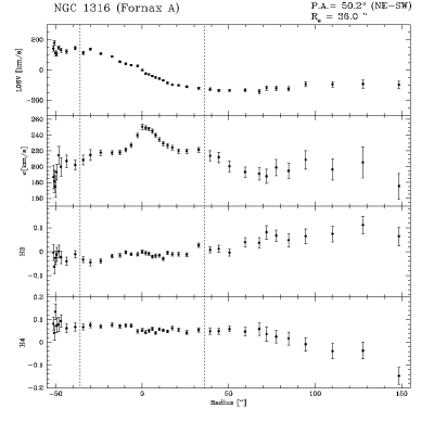
Figure 5: The major-axis kinematics of NGC 1316.

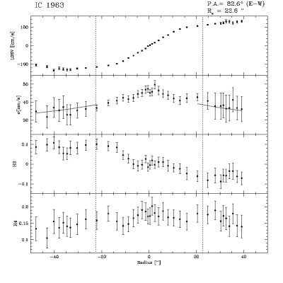
Figure 8: The major-axis kinematics of IC 1963.

References

- (1) Andreon S., 1998, ApJ, 501, 533
- (2) Bekki K., 1998, ApJ, 502, L133
- (3) Bekki K., Shioya Y., Couch W.J, 2002, ApJ, 577, 651
- (4) Bernardi M., Alonso M.V., Da Costa L.M., Willmer C.N.A., Wegner G., Pellegrini P.S., Reté C., Maia M.A.G., 2002, AJ, 123, 2990B
- (5) Bertola F., Buson L. M., Zeilinger W. W., 1992, ApJ, 401L, 79B
- (6) Binney J., Tremaine S., 1987, “Galactic Dynamics”, Princeton Series in Astrophysics
- Brown (2001) Brown T., 2001, Instrument Science Report STIS 2001-005
- Bureau, Athanassoula (2005) Bureau M., Athanassoula E., 2005, ApJ, 626, 159
- (9) Caon N., Capaccioli M., D’Onofrio M., 1994, A&AS, 106, 199
- Cappellari, Emsellem (2004) Cappellari M., Emsellem E., 2004, PASP, 116, 138
- (11) Christlein D., Zabludoff A.I., 2004, ApJ, 616, 192C
- (12) De Vaucouleurs, G., de Vaucouleurs A., Corwin H. G., Buta R. J., Paturel G., Fouque, P. 1991, Volume 1-3, XII, Springer-Verlag Berlin Heidelberg New York,
- (13) Desai et al., 2006, submitted.
- (14) D’Onofrio M., Zaggia S.R., Longo G., Caon N., Capaccioli M., 1995, A&A, 296, 319
- (15) Dressler A. 1980, ApJ, 236, 351 217, 493
- (16) Dressler A., et al., 1997, ApJ, 490, 577
- (17) Emsellem E., Cappellari M., Peletier R.F., et al., 2004, MNRAS, 352, 721
- (18) Fasano G., Poggianti B. M., Couch W. J., Bettoni D., Kjærgaard P., Moles M. 2000, ApJ, 542, 673
- (19) Freeman K.C., 1970, ApJ, 160, 811F
- (20) Goto T., et al., 2003, PASJ, 55, 757
- (21) Graham A.W., Colless M.M., Busarello G., Zaggia S., Longo G., 1998, A&AS, 133, 325
- (22) Gunn J.E., Gott J.R., 1972, ApJ, 176, 1
- (23) Hernquist L., 1990, ApJ, 356, 359
- (24) Hinz J.L., Rix H.,-W., Bernstein G.M., 2001, AJ, 121, 683
- (25) Hinz J.L., Rieke G.H., Caldwell N., 2003, AJ, 126, 2622
- (26) Jorgensen I., Franx M., 1994, ApJ, 433, 553
- (27) Jarret T.H., 2000, PASP, 112, 1008J
- (28) Jarret T.H., Chester T., Cutri R., Schneider S.E., Huchra J.P., 2003, AJ, 125, 525J
- (29) Kuijken K., Merrifield M.R., 1995, ApJ, 443, L13
- (30) Kissler-Patig M., 1997, A&A, 319, 83
- (31) Kuntschner H., 2000, MNRAS, 315, 184K
- (32) Larson R.B., Tinsley B.M., Caldwell C.N., 1980, ApJ, 237, 692L
- (33) Longhetti M., Rampazzo R., Bressan A., Chiosi C., 1998, A&AS, 130, 267L
- (34) Lorenz H., Böhm P., Capaccioli M., Richter G.M., Longo G., 1993, A&AS, 277, L15
- (35) Madore B.F., Freedman W.C., Silbermann, N., et al., 1999, ApJ, 515, 29
- (36) Mathieu A., Merrifield M., Kuijken K., 2002, MNRAS, 330, 251
- (37) Mehlert D., Saglia R.P., Bender R., Wegner G., 2000, A&AS, 141, 449
- (38) Mehlert D., Thomas D., Saglia R.P., Bender R., Wegner G., 2003, A&A, 407, 423
- (39) Merrett H.R., Merrifield M.R., Douglas N.G., et al., 2006, astro-ph/0603125
- (40) Merrifield M., Fisher D., Kuijken K., 1996, AAS, 189.5405M
- (41) Mihos J.C., Hernquist L., 1994, ApJ, 425, L13
- Moore et al. (1998) Moore B., Lake G.,, Katz N., 1998, ApJ, 495, 139
- Moss, Whittle (2000) Moss C., Whittle M., 2000, MNRAS, 317 667
- (44) Neistein E., Maoz D., Rix H.-W., Tonry J.L., 1999, AJ, 117, 2666
- (45) Nieto J.-L., Bender R., Surma P., 1991, A&A, 244, 37N
- (46) Rubin V., Graham J.A., Kenney, J.D.P., 1992, ApJ, 394, L9
- (47) Poggianti B., Bridges T.J., Carter D. et al. 2001a, ApJ 563, 118
- (48) Shioya Y., Bekki K., Couch W.J., 2004, ApJ, 601, 654
- Simard (2002) Simard L., Willmer C.N.A., Vogt N.P. et al., 2002, ApJS, 142, 1S
- (50) Sandage A., Tammann G.A., 1987, A Revised Catalog of Shapley-Ames Galaxies (2d ed.; Washington:Carnegie Institution)
- (51) Smail I., Kuntschner H., Kodama T., et al., 2001, MNRAS, 323, 839 217, 493
- (52) Tody D., 1986, “The IRAF Data Reduction and Analysis System”, in proc. SPIE Instrumentation in Astronomy VI, ed. D. L. Crawford, 627, 733
- (53) Tody D., 1993, “IRAF in the Nineties”, in Astronomical Data Analysis Software and Systems II, A.S.P. Conference Ser., Vol 52, eds. R.J. Hanisch, R.J.V. Brissenden, J. Barnes, 173
- (54) Van den Bergh S., 1990, ApJ, 348, 57