Clustering of $i_{775}$ dropout galaxies at $z\sim 6$ in GOODS and the UDF

Abstract

We measured the angular clustering at $z\sim 6$ from a large sample of $i_{775}$ dropout galaxies (293 with $z_{850}$$\leq$27.5 from GOODS and 95 with $z_{850}$$\leq$29.0 from the UDF). Our largest and most complete subsample (having $L\gtrsim 0.5L^{*}_{z=6}$) shows the presence of clustering at 94% significance. For this sample we derive a (co-moving) correlation length of $r_{0}=4.5^{+2.1}_{-3.2}$ $h_{72}^{-1}$ Mpc and bias $b=4.1^{+1.5}_{-2.6}$, using an accurate model for the redshift distribution. No clustering could be detected in the much deeper but significantly smaller UDF, yielding $b<4.4$ (1$\sigma$). We compare our findings to Lyman break galaxies at $z\sim 3-5$ at a fixed luminosity. Our best estimate of the bias parameter implies that $i_{775}$ dropouts are hosted by dark matter halos having masses of $\sim 10^{11}$ $M_{\odot}$, similar to that of $V_{606}$ dropouts at $z\sim 5$. We evaluate a recent claim that at $z\gtrsim 5$ star formation might have occurred more efficiently compared to that at $z=3-4$. This may provide an explanation for the very mild evolution observed in the UV luminosity density between $z=6$ and 3. Although our results are consistent with such a scenario, the errors are too large to find conclusive evidence for this.

1. Introduction

The Advanced Camera for Surveys (ACS; Ford et al., 1998) aboard the Hubble Space Telescope has made the detection of star-forming galaxies at $z\sim 6$ ($i_{775}$ dropouts) relatively easy. The largest sample of $i_{775}$ dropouts currently available (Bouwens et al., 2006) comes from the Great Observatories Origins Deep Survey (GOODS; Giavalisco et al., 2004), allowing the first quantitative analysis of galaxies only 0.9 Gyr after recombination (Stanway et al., 2003; Bouwens et al., 2003; Yan & Windhorst, 2004; Dickinson et al., 2004; Malhotra et al., 2005, see also Shimasaku et al. 2005; Ouchi et al. 2005b). Bouwens et al. (2006) found evidence for strong evolution of the luminosity function between $z\sim 6$ and 3, while the (unextincted) luminosity density at $z\sim 6$ is only $\sim 0.8$ times lower than that at $z\sim 3$. Some $i_{775}$ dropouts have significant Balmer breaks, indicative of stellar populations older than 100 Myr and masses comparable to those of $L^{*}$ galaxies at $z\approx 0$ (Eyles et al., 2005; Yan et al., 2005).

Through the study of the clustering we can address fundamental cosmological issues that cannot be answered from the study of galaxy light alone. The strength of clustering and its evolution with redshift allows us to relate galaxies with the underlying dark matter and study the bias. The two-point angular correlation function (ACF) has been used to measure the clustering of Lyman break galaxies (LBGs) at $z=3-5$ (e.g., Adelberger et al., 1998, 2005; Arnouts et al., 1999, 2002; Magliocchetti & Maddox, 1999; Giavalisco & Dickinson, 2001; Ouchi et al., 2001, 2004; Porciani & Giavalisco, 2002; Hildebrandt et al., 2005; Allen et al., 2005; Kashikawa et al., 2006). LBGs are highly biased ($b\simeq 2-8$), and this biasing depends strongly on rest frame UV luminosity and, to a lesser extent, on dust and redshift. The clustering statistics of LBGs have reached the level of sophistication that one can measure two physically different contributions. At small angular scales the ACF is dominated by the non-linear clustering of galaxies within single dark matter halos, whereas at large scales its amplitude tends to the “classical” clustering of galaxies residing in different halos (Ouchi et al., 2005a; Lee et al., 2006), as explained within the framework of the halo occupation distribution (e.g., Zehavi et al., 2004; Hamana et al., 2004). Understanding the clustering properties of galaxies at $z\sim 6$ is important for the interpretation of “overdensities” observed towards luminous quasars and in the field (Ouchi et al., 2005b; Stiavelli et al., 2005; Wang et al., 2005; Zheng et al., 2006) that could demarcate structures that preceded present-day massive galaxies and clusters (Springel et al., 2005). Our aim here is to “complete” the census of clustering by extending it to the highest redshift regime with sizeable samples. In §§ 2 and 3 we describe the sample, and present our measurements of the ACF. In § 4 we discuss our findings. Throughout we use the cosmology ($\Omega_{M}$, $\Omega_{\Lambda}$, $h_{72}$, $n$, $\sigma_{8}$)$=$(0.27,0.73,1.0,1.0,0.9) with $H_{0}=72$ $h_{72}$ km s^-1 Mpc^-1.

Figure 1.— Redshift distributions of $i_{775}$ dropouts in our GOODS (left) and UDF (right) selections (estimated by projecting a complete UDF $B_{435}$ dropout sample scaled to the sizes and colors as found for the $i_{775}$ dropout sample to $z\sim 5-7$; see Bouwens et al., 2006, for details). As a result of a more significant photometric scatter in $i_{775}$–$z_{850}$, the selection extends to lower redshifts in GOODS than it does for the UDF.

2. Data

The present analysis is based on the sample of $i_{775}$ dropouts described in detail by Bouwens et al. (2006). We used the ACS data from the GOODS v1.0 release, consisting of two spatially disjoint, $\sim 160$ arcmin² fields. These data were processed with Apsis (Blakeslee et al., 2003), along with a substantial amount of overlapping data available from the Galaxy Evolution from Morphology and Spectral energy distributions (GEMS; Rix et al., 2004), supernova searches (A. G. Riess et al. 2006 and S. Perlmutter et al. 2006, both in preparation), and Ultra Deep Field (UDF) NICMOS programs (Thompson et al., 2005). The processed images were brought to a uniform signal-to-noise level by degrading the deeper parts of the area. The $10\sigma$ detection limit of the degraded data was 27.5 in $z_{850}$ in a $0\farcs 2$ diameter aperture. We also used a deep sample of $i_{775}$ dropouts selected from the UDF (Beckwith et al., 2006), covering one ACS pointing of $\sim 11$ arcmin² with a 10$\sigma$ detection limit of 29.2.

Objects were selected by requiring $i_{775}$–$z_{850}$$>$1.3, and $V_{606}$–$z_{850}$$>$2.8 or a non-detection (2$\sigma$) in $V_{606}$ to exclude lower redshift interlopers. Point sources were removed based on high stellarity parameters $>$0.75. The estimated residual contamination due to photometric scatter, red interlopers, and stars is $\sim$7% to $z_{850}$$=$28.0, of which 2% is due to stars (see Bouwens et al., 2006, for details). The effective redshift distributions for GOODS and the UDF are shown in Figure 1. The effective rest-frame UV luminosity of the sample is $L\approx 0.5L^{*}_{z=6}$ for $z_{850}$$\sim$27.5 (Bouwens et al., 2006). Note that the luminosity is quite sensitive to redshift due to the Gunn-Peterson trough entering $z_{850}$ at $z>6$, with $L^{*}_{z=6}$ corresponding to $z_{850}$$\sim$26.5 ($\sim$28) at $z=5.5$ ($z=6.5$).

3. The angular correlation function

We measured the ACF, $w(\theta)$, defined as the excess probability of finding two sources in the solid angles $\delta\Omega_{1}$ and $\delta\Omega_{2}$ separated by the angle $\theta$, over that expected for a random Poissonian distribution (Peebles, 1980). We used the estimator $w(\theta)=[DD(\theta)-2DR(\theta)+RR(\theta)]/RR(\theta)$ of Landy & Szalay (1993), where $DD(\theta)$, $DR(\theta)$ and $RR(\theta)$ are the number of pairs of sources with angular separations between $\theta$ and $\theta$$+$$\Delta\theta$ measured in the data, random, and data-random cross catalogs, respectively. We used 16 random catalogs containing $\sim 100$ times more sources than in the data, but with a similar angular geometry. Errors on $w(\theta)$ were bootstrapped (Ling et al., 1986). We assumed a power-law ACF of the form $w(\theta)$$=$$A_{w}\theta^{-\beta}$ and determined its amplitude, $A_{w}$, by fitting the function $w(\theta)$$=$$A_{w}\theta^{-\beta}$$-$$IC$. The integral constraint [$IC$$=$$\int\int w(\theta)d\Omega_{1}d\Omega_{2}/\Omega^{2}$, where $\Omega$ is the survey area] was $0.033A_{w}$ for GOODS and $0.074A_{w}$ for the UDF. We did not attempt to fit the slope of the ACF and assumed $\beta=0.6$ based on the results of Lee et al. (2006). The ACF was fitted over the range 10″–300″ (10″–200″ for the UDF), corresponding to roughly 0.4–10 $h_{72}^{-1}$ Mpc comoving at $z\sim 6$. The lower value of 10″ is larger than the virial radius of a $10^{12}$ $M_{\odot}$ halo to ensure that we are measuring the large-scale clustering (and not receiving a contribution at small scales from the subhalo component). Because the results of the fits are sensitive to the size of the bins used, we determined $A_{w}$ using Monte Carlo simulations of the data. Finally, we note that if the contaminants to our samples ($\sim$7% of the total) have a uniform distribution, the measured amplitude should be multiplied by $\sim$1.16 to yield the corrected clustering amplitude.

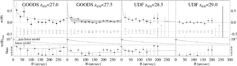
Figure 2.— Top panels show the measurements (points) and the best-fit ACF (solid line) for the $i_{775}$ dropout samples extracted from GOODS and the UDF. The slope was kept fixed at $\beta=0.6$. Shot noise expectations have been indicated by empty error bars (offset by –0.4 in the vertical direction for clarity). The middle and bottom panels show, respectively, the (non)linear clustering of dark matter (Peacock & Dodds, 1996) and the bias at each $\theta$ (points) and for the best-fit ACF (solid line). The hatched region indicates the $1\sigma$ range of $w(\theta)$ expected based on a simulated distribution with the same clustering amplitude as measured for the $z_{850}$$<$27.5 sample.

3.1. Results from GOODS and the UDF

Figure 2 (top panels) shows the GOODS and UDF ACFs for various limiting magnitudes. The results of the fits are given in Table 1. For the three brightest subsamples ($z_{850}$$<$28.5) we measured a positive signal out to $\theta\sim 1\arcmin$. In GOODS, we found $A_{w}=2.71\pm 2.05$ for $z_{850}$$<$27.0, and $A_{w}\approx 0.80\pm 0.69$ for $z_{850}$$<$27.5. The analysis of the UDF is hampered by the relatively small number of sources available, owing to its $\sim 30$ times smaller area, although its greater depth (1.5 mag) partially makes up for this lack of area. We found $A_{w}=1.40\pm 1.64$ and $A_{w}=0.00\pm 0.93$ for the $z_{850}$$<$28.5 and $z_{850}$$<$29.0 samples, respectively.

Because the objects were selected from data of uniform depth, signal in the ACF is unlikely to be caused by variations in the object surface density. Given the large errors on $A_{w}$, it is useful to ask whether the $w(\theta)$ observed at $\theta\lesssim 1\arcmin$ could be the result of shot noise in a random object distribution. We created 1000 random distributions with the same geometry and the same number of points as our GOODS and UDF data, and calculated the ACF in each of the random samples. The mean and standard deviation at each $\theta$ is plotted in Figure 2 (top panels, offset by –0.4 for clarity). We calculate the chance of reproducing the observed clustering in the random realizations, using the average $w(\theta)$ measured over the first four bins ($\theta<100\arcsec$) as a gauge of this clustering. This chance is 0.1% for our $z_{850}$$<$27.0 sample, and 6%, 10% and 35% for the fainter samples.

Table 1ACF and related physical quantities.

$z_{850}$		Area	$A_{w}$	$r_{0}$
(mag)	$N$($<$$z$)	(arcmin2)	(arcsecβ)	($h_{72}^{-1}$ Mpc)	$b$ (30″)
Enhanced GOODS Data
27.0 ……	172	$2\times 160$	$2.71\pm 2.05$	$9.6^{+4.0}_{-5.6}$	$7.5^{+2.5}_{-3.8}$
27.5 ……	293	$2\times 160$	$0.80\pm 0.69$	$4.5^{+2.1}_{-3.2}$	$4.1^{+1.5}_{-2.6}$
UDF Data
28.5 ……	52	$1\times 11$	$1.40\pm 1.64$	$<10.2$	$<8.0$
29.0 ……	95	$1\times 11$	$0.00\pm 0.93$	$<4.8$	$<4.4$

Another test of the clustering signal detected in this sample was as follows. We used the formalism of Soneira & Peebles (1978) to create mock samples with a choice ACF in two dimensions. A $250\arcmin\times 250\arcmin$ mock field with surface density similar to that of the $i_{775}$ dropouts allowed us to mimic the measured $A_{w}$ to an accuracy of $\>98$%, determined from a fit. Next, we randomly extracted 100 mock “GOODS” surveys and measured the mean $w(\theta)$ and its standard deviation using identical binning and fitting to that for the real samples. The result is indicated in Figure 2 (hatched region) for our $z_{850}$$<$27.5 sample, which being our largest and most complete sample provides the most reliable constraint on this clustering. The simulation demonstrates that the amplitude of the observed $w(\theta)$ at $\theta\lesssim 1\arcmin$ lies within $\lesssim 1\sigma$ of the amplitudes predicted based on our model ACF, although the scatter in the expected amplitudes is large.

In the above analysis we restricted ourselves to clustering at $\theta$$\geq$10″. Our measurements also showed an excess of pair counts at $\theta$$<$10″. Upon closer inspection it was found that the excess was strictly limited to $\theta$$<$5″, with $w(2\farcs 5)$$\sim$$2.0\pm 0.9$. The excess is consistent with an enhancement of $w(\theta)$ due to subhalo clustering at $\lesssim 30$ kpc to $1.7\sigma$ confidence, but the exact amplitude cannot be determined accurately due to the small number of pairs (11 pairs at $z_{850}$$<$28.0). The excess is similar to that found for Ly$\alpha$ emitters at $z=5.7$ (Shimasaku et al., 2006). While it is possible that the positive signal out to $\sim 1$′ is the result of strong subhalo clustering (see Lee et al., 2006; Ouchi et al., 2005b), the occurrence of such halos becomes increasingly rare with redshift, and by limiting the fits to $\theta\gtrsim$10″ we minimized any contribution.

4. Derivation of cosmological quantities

Although the uncertainties are large, we estimate the spatial correlation length ($r_{0}$) from $A_{w}$, using the Limber equation adopted for our cosmology and the redshift distributions of Figure 1 (see Table 1). The clustering was assumed to be fixed in comoving coordinates across the redshift range. We found $r_{0}$$=$4.5${}^{+2.1}_{-3.2}$ $h_{72}^{-1}$ Mpc for the $z_{850}$$<$27.5 sample. At $z_{850}$$<$27, the best-fit value was found to be twice as high, $r_{0}$$=$9.6${}^{+4.0}_{-5.6}$ $h_{72}^{-1}$ Mpc, but consistent with the fainter subsample within the errors. For the UDF samples, the best-fit values correspond to upper limits for the clustering amplitude of $\sim 10$ and $\sim 5$ $h_{72}^{-1}$ Mpc for $z_{850}$$<$28.5 and $z_{850}$$<$29, respectively. If we apply the contamination correction, $r_{0}$ increases by $\sim$10%.

We calculated the galaxy–dark matter bias, defined as $b(\theta)$$\equiv$$\sqrt{w(\theta)/w_{dm}(\theta)}$, where $w_{dm}(\theta)$ is the ACF of the dark matter as “seen” through our redshift window; $w_{dm}(\theta)$ was calculated using the nonlinear fitting function of Peacock & Dodds (1996) (Fig. 2, middle panels). In the bottom panels of Figure 2 we have indicated the bias as a function of $\theta$ (points). Our best-fit ACF at $z_{850}$$<$27.5 implies $b(\theta$$\sim$30$\arcsec)$$=$$4.1^{+1.5}_{-2.6}$ (solid line), bracketed by $b\sim 8$ for the brightest GOODS sample and $b<4.4$ for the faintest UDF sample. The contamination correction yields values that are $\sim$5% higher.

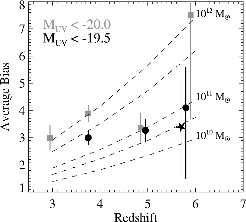
Figure 3.— Bias of $i_{775}$ dropouts compared to bias at $z=3-5$ from Lee et al. (2006). Dashed lines indicate the bias of dark halos from Sheth & Tormen (1999) for $M_{halo}\geq 10^{10}$, $5\times 10^{10}$, $10^{11}$, $5\times 10^{11}$, and $10^{12}$ $M_{\odot}$ (bottom to top). The relatively small halo mass inferred at $z=5$ compared to that at $z=4$ for objects with $M_{z}\lesssim-20$ (squares) cannot be confirmed at $z=6$ based on the present data. The best-fit halo mass inferred for objects at $z=6$ is consistent with the average halo mass of $V_{606}$ dropouts at $z=5$ at a fixed luminosity of $M_{z}<-19.5$ (circles). The star indicates the bias of Ly$\alpha$ emitters at $z=5.7$ from Ouchi et al. (2005b).

It is important to evaluate how our results might be influenced by cosmic variance. Using Somerville et al. (2004), we estimate $\sigma_{v}$$\sim$0.2 for GOODS and $\sigma_{v}$$\sim$0.5 for the UDF ($\sigma_{v}$ being the square root of the cosmic variance). Our best constraint on clustering at $z=6$ is therefore currently provided by the $z_{850}$$<$27.5 sample, given the relatively small variance, large sample size, and large completeness. Our best value for the bias of $i_{775}$ dropouts is very similar to the bias of $b=3.4\pm 1.8$ found for faint Ly$\alpha$ emitters in the Subaru/XMM-Newton Deep Field (Ouchi et al., 2005b). An alternative method of estimating the bias is to directly compare the $i_{775}$ dropout number density to the number density of dark halos at $z=6$. Assuming that the bias of the $i_{775}$ dropouts corresponds to that of dark halos more massive than the average halo hosting them (Sheth & Tormen, 1999), following Somerville et al. (2004) we predict that the average bias ranges from $b\approx 5.5$ to $b\approx 3.8$ for samples with limiting magnitudes from $z_{850}$$=$27 to $z_{850}$$=$29, with $\sim$5% errors in these estimates due to the uncertainty in number density caused by cosmic variance. These values are largely in agreement with our measurements. The model predictions furthermore suggest that our best-fit value measured for the brightest GOODS sample ($z_{850}$$<$27.0) is likely spuriously high, given that the number density changes by not more than a factor of 2 over half a magnitude, giving only a modest increase in the bias compared to the $z_{850}$$<$27.5 sample. This GOODS sample thus adds very little additional constraints to the clustering at $z=6$. The UDF samples suffer from relatively small number statistics, as well as large cosmic variance. The clustering signal in the UDF is likely further diminished due to the strong luminosity dependence of clustering as seen at lower redshift (e.g., Kashikawa et al., 2006).

In Figure 3 we compare our results to the work of Lee et al. (2006), who found $b$$\approx$3.3$\pm$0.5 for faint $V_{606}$ dropouts ($z\sim 5$) also selected from GOODS. At $z_{850}$$\sim$27.5 we probe approximately the same rest-frame luminosity as their faintest (i.e., $z_{850}$$\leq$27) $V_{606}$ dropout sample ($M_{z}\lesssim-19.5$). To this limit, we measure a bias of $b=4.1^{+1.5}_{-2.6}$, suggesting an average halo mass of $\simeq 10^{11}$ $M_{\odot}$, comparable to the average mass of halos hosting $V_{606}$ dropouts.

Interestingly, Lee et al. (2006) found that at slightly higher rest-frame luminosities ($M_{z}\lesssim-20$), the clustering of $V_{606}$ dropouts is weaker than that of $U$ and $B_{435}$ dropouts at $z=3-4$. It is hence inferred that the halo mass at $z=3-4$ is $\sim 10$ times larger ($\sim$10¹² $M_{\odot}$) compared to that at $z=5$ (see Fig. 3). Lee et al. (2006) argued that star formation occurred more efficiently at higher redshifts ($z\sim 5$) than it did at $z\sim 3-4$, given that objects of comparable luminosity are found in less massive halos at $z\sim 5$. Unfortunately, this result cannot be confirmed at $z\sim 6$ using our brightest ($M_{z}\lesssim-20$) GOODS sample, given the large uncertainties in the bias and the associated halo mass. Also, the decrease in the effective halo mass from $z=4$ to 5 at $M_{z}\lesssim-19.5$ is not as dramatic as observed at luminosities of $M_{z}\lesssim-20$, making it difficult to verify this result based on the present $i_{775}$ dropout sample. However, we note that if a decrease in the star-forming efficiency with decreasing redshift is true (and can be confirmed for galaxies at $z\gtrsim 6$), it would largely offset changes that are occurring in the mass function over this range. As such, this may provide at least a partial explanation for the mild evolution in the luminosity density from $z=6$ to 3.

In conclusion, we used the largest available sample of $i_{775}$ dropouts to study clustering at $z\sim 6$. We found a small signal, although its amplitude is not well constrained due to the large errors on the individual datapoints. The present analysis is therefore reminiscent of that performed at $z\sim 3-5$ based on the original Hubble Deep Fields. The clustering of galaxies at $z\sim 6$ will continue to be studied from deep, wide surveys (e.g., see Ouchi et al., 2005b; Shimasaku et al., 2005, 2006). Although it might become possible in the near future to increase the size of our faint ACS samples by relaxing our current $i_{775}$ dropout detection threshold, to perform an analysis at the same level of detail as currently performed at $z\sim 5$ would require another six GOODS fields, for $\sim$1200 arcmin² in total.

References

- Adelberger et al. (1998) Adelberger, K. L., Steidel, C. C., Giavalisco, M., Dickinson, M., Pettini, M., & Kellogg, M. 1998, ApJ, 505, 18
- Adelberger et al. (2005) Adelberger, K. L., Steidel, C. C., Pettini, M., Shapley, A. E., Reddy, N. A., & Erb, D. K. 2005, ApJ, 619, 697
- Allen et al. (2005) Allen, P. D., Moustakas, L. A., Dalton, G., MacDonald, E., Blake, C., Clewley, L., Heymans, C., & Wegner, G. 2005, MNRAS, 360, 1244
- Arnouts et al. (1999) Arnouts, S., Cristiani, S., Moscardini, L., Matarrese, S., Lucchin, F., Fontana, A., & Giallongo, E. 1999, MNRAS, 310, 540
- Arnouts et al. (2002) Arnouts, S. et al. 2002, MNRAS, 329, 355
- Beckwith et al. (2006) Beckwith, S. V. W., et al. 2006, AJ, 132, 1729
- Blakeslee et al. (2003) Blakeslee, J. P., Anderson, K. R., Meurer, G. R., Benítez, N., & Magee, D. 2003, in ASP Conf. Ser. 295: Astronomical Data Analysis Software and Systems XII, 257
- Bouwens et al. (2003) Bouwens, R., Broadhurst, T., & Illingworth, G. 2003, ApJ, 593, 640
- Bouwens et al. (2006) Bouwens, R. J., Illingworth, G. D., Blakeslee, J. P., & Franx, M. 2006, ApJ, In Press (astro-ph/0509641)
- Dickinson et al. (2004) Dickinson, M. et al. 2004, ApJ, 600, L99
- Eyles et al. (2005) Eyles, L. P., Bunker, A. J., Stanway, E. R., Lacy, M., Ellis, R. S., & Doherty, M. 2005, MNRAS, 364, 443
- Ford et al. (1998) Ford, H. C. et al. 1998, in Proc. SPIE Vol. 3356, p. 234-248, Space Telescopes and Instruments V, Pierre Y. Bely; James B. Breckinridge; Eds., 234–248
- Giavalisco & Dickinson (2001) Giavalisco, M., & Dickinson, M. 2001, ApJ, 550, 177
- Giavalisco et al. (2004) Giavalisco, M. et al. 2004, ApJ, 600, L93
- Hamana et al. (2004) Hamana, T., Ouchi, M., Shimasaku, K., Kayo, I., & Suto, Y. 2004, MNRAS, 347, 813
- Hildebrandt et al. (2005) Hildebrandt, H. et al. 2005, A&A, 441, 905
- Kashikawa et al. (2006) Kashikawa, N. et al. 2006, ApJ, 637, 631
- Landy & Szalay (1993) Landy, S. D., & Szalay, A. S. 1993, ApJ, 412, 64
- Lee et al. (2006) Lee, K.-S., Giavalisco, M., Gnedin, O. Y., Somerville, R. S., Ferguson, H. C., Dickinson, M., & Ouchi, M. 2006, ApJ, 642, 63
- Ling et al. (1986) Ling, E. N., Barrow, J. D., & Frenk, C. S. 1986, MNRAS, 223, 21P
- Magliocchetti & Maddox (1999) Magliocchetti, M., & Maddox, S. J. 1999, MNRAS, 306, 988
- Malhotra et al. (2005) Malhotra, S., et al. 2005, ApJ, 626, 666
- Ouchi et al. (2001) Ouchi, M., et al. 2001, ApJ, 558, L83
- Ouchi et al. (2005a) Ouchi, M. et al. 2005a, ApJ, 635, L117
- Ouchi et al. (2005b) Ouchi, M. et al. 2005b, ApJ, 620, L1
- Ouchi et al. (2004) Ouchi, M., et al. 2004, ApJ, 611, 685
- Peacock & Dodds (1996) Peacock, J. A., & Dodds, S. J. 1996, MNRAS, 280, L19
- Peebles (1980) Peebles, P. J. E. 1980, The large-scale structure of the universe (Princeton University Press)
- Porciani & Giavalisco (2002) Porciani, C., & Giavalisco, M. 2002, ApJ, 565, 24
- Rix et al. (2004) Rix, H.-W. et al. 2004, ApJS, 152, 163
- Sheth & Tormen (1999) Sheth, R. K., & Tormen, G. 1999, MNRAS, 308, 119
- Shimasaku et al. (2005) Shimasaku, K., Ouchi, M., Furusawa, H., Yoshida, M., Kashikawa, N., & Okamura, S. 2005, PASJ, 57, 447
- Shimasaku et al. (2006) Shimasaku, K. et al. 2006, PASJ, 58, 313
- Somerville et al. (2004) Somerville, R. S., Lee, K., Ferguson, H. C., Gardner, J. P., Moustakas, L. A., & Giavalisco, M. 2004, ApJ, 600, L171
- Soneira & Peebles (1978) Soneira, R. M., & Peebles, P. J. E. 1978, AJ, 83, 845
- Springel et al. (2005) Springel, V. et al. 2005, Nature, 435, 629
- Stanway et al. (2003) Stanway, E. R., Bunker, A. J., & McMahon, R. G. 2003, MNRAS, 342, 439
- Stiavelli et al. (2005) Stiavelli, M. et al. 2005, ApJ, 622, L1
- Thompson et al. (2005) Thompson, R. I. et al. 2005, AJ, 130, 1
- Wang et al. (2005) Wang, J. X., Malhotra, S., & Rhoads, J. E. 2005, ApJ, 622, L77
- Yan et al. (2005) Yan, H. et al. 2005, ApJ, 634, 109
- Yan & Windhorst (2004) Yan, H., & Windhorst, R. A. 2004, ApJ, 612, L93
- Zehavi et al. (2004) Zehavi, I. et al. 2004, ApJ, 608, 16
- Zheng et al. (2006) Zheng, W. et al. 2006, ApJ, 640, 574